Sharper Sub-Weibull Concentrations

Abstract

Constant-specified and exponential concentration inequalities play an essential role in the finite-sample theory of machine learning and high-dimensional statistics area. We obtain sharper and constants-specified concentration inequalities for the sum of independent sub-Weibull random variables, which leads to a mixture of two tails: sub-Gaussian for small deviations and sub-Weibull for large deviations from the mean. These bounds are new and improve existing bounds with sharper constants. In addition, a new sub-Weibull parameter is also proposed, which enables recovering the tight concentration inequality for a random variable (vector). For statistical applications, we give an ${\ell }_2$-error of estimated coefficients in negative binomial regressions when the heavy-tailed covariates are sub-Weibull distributed with sparse structures, which is a new result for negative binomial regressions. In applying random matrices, we derive non-asymptotic versions of Bai-Yin’s theorem for sub-Weibull entries with exponential tail bounds. Finally, by demonstrating a sub-Weibull confidence region for a log-truncated Z-estimator without the second-moment condition, we discuss and define the sub-Weibull type robust estimator for independent observations ${\left\{X_i\right\}}_{i=1}^n$ without exponential-moment conditions.

1. Introduction

In the last two decades, with the development of modern data collection methods in science and techniques, scientists and engineers can access and load a huge number of variables in their experiments. Over hundreds of years, probability theory lays the mathematical foundation of statistics. Arising from data-driving problems, various recent statistics research advances also contribute to new and challenging probability problems for further study. For example, in recent years, the rapid development of high-dimensional statistics and machine learning have promoted the development of the probability theory and even pure mathematics, such as random matrices, large deviation inequalities, and geometric functional analysis, etc.; see [1]. More importantly, the concentration inequality (CI) quantifies the concentration of measures that are at the heart of statistical machine learning. Usually, CI quantifies how a random variable (r.v.) X deviates around its mean $\mathrm{E}X=:\mu$ by presenting as one-side or two-sided bounds for the tail probability of $X-\mu$

$$\mathrm{P}(X-\mu >t)\mathrm{or}\mathrm{P}(|X-\mu |>t)\le \mathrm{some}\mathrm{small}\delta ,\forall t\ge 0.$$

The classical statistical models are faced with fixed-dimensional variables only. However, contemporary data science motivates statisticians to pay more attention to studying $p\times p$ random Hessian matrices (or sample covariance matrices, [2]) with $p\to \infty$, arising from the likelihood functions of high-dimensional regressions with covariates in ${\mathbb{R}}^p$. When the model dimension increases with sample size, obtaining asymptotic results for the estimator is potentially more challenging than the fixed dimensional case. In statistical machine learning, concentration inequalities (large derivation inequalities) are essential in deriving non-asymptotic error bounds for the proposed estimator; see [3,4]. Over recent decades, researchers have developed remarkable results of matrix concentration inequalities, which focuses on non-asymptotic upper and lower bounds for the largest eigenvalue of a finite sum of random matrices. For a more fascinated introduction, please refer to the book [5].

Motivated from sample covariance matrices, a random matrix is a specific matrix ${\mathbf{A}}_{p\times p}$ with its entries $A_{jk}$ drawn from some distributions. As $p\to \infty$, random matrix theory mainly focuses on studying the properties of the p eigenvalues of ${\mathbf{A}}_{p\times p}$, which turn out to have some limit law. Several famous limit laws in random matrix theory are different from the CLT for the summation of independent random variables since the p eigenvalues are dependent and interact with each other. For convergence in distribution, some pioneering works are the Wigner’s semicircle law for some symmetric Gaussian matrices’ eigenvalues, the Marchenko-Pastur law for Wishart distributed random matrices (sample covariance matrices), and the Tracy-Widom laws for the limit distribution for maximum eigenvalues in Wishart matrices. All these three laws can be regarded as the CLT of random matrix versions. Moreover, the limit law for the empirical spectral density is some circle distribution, which sheds light on the non-communicative behaviors of the random matrix, while the classic limit law in CLT is for normal distribution or infinite divisible distribution. For strong convergence, Bai-Yin’s law complements the Marchenko-Pastur law, which asserts that almost surely convergence of the smallest and largest eigenvalue for a sample covariance matrix. The monograph [2] thoroughly introduces the limit law in random matrices.

This work aims to extend non-asymptotic results from sub-Gaussian to sub-Weibull in terms of exponential concentration inequalities with applications in count data regressions, random matrices, and robust estimators. The contributions are:

(i)

We review and present some new results for sub-Weibull r.v.s, including sharp concentration inequalities for weighted summations of independent sub-Weibull r.v.s and negative binomial r.v.s, which are useful in many statistical applications.

(ii)

Based on the generalized Bernstein-Orlicz norm, a sharper concentration for sub-Weibull summations is obtained in Theorem 1. Here we circumvent Stirling’s approximation and derive the inequalities more subtly. As a result, the confidence interval based on our result is sharper and more accurate than that in [6] (For example, see Remark 2) and [7] (see Proposition 1 with unknown constants) gave.

(iii)

By sharper sub-Weibull concentrations, we give two applications. First, from the proposed negative binomial concentration inequalities, we obtain the $O_P\left(\sqrt{p/n}\right)$ (up to some log factors) estimation error for the estimated coefficients in negative binomial regressions under the increasing-dimensional framework $p=p_n$ and heavy-tailed covariates. Second, we provide a non-asymptotic Bai-Yin’s theorem for sub-Weibull random matrices with exponential-decay high probability.

(iv)

We propose a new sub-Weibull parameters, which is enabled of recovering the tight concentration inequality for a single non-zero mean random vector. The simulation studies for estimating sub-Gaussian and sub-exponential parameters show these parameters could be estimated well.

(v)

We establish a unified non-asymptotic confidence region and the convergence rate for general log-truncated Z-estimator in Theorem 5. Moreover, we define a sub-Weibull type estimator for a sequence of independent observations ${\left\{X_i\right\}}_{i=1}^n$ without the second-moment condition, beyond the definition of the sub-Gaussian estimator.

2. Sharper Concentrations for Sub-Weibull Summation

Concentration inequalities are powerful in high-dimensional statistical inference, and it can derive explicit non-asymptotic error bounds as a function of sample size, sparsity level, and dimension [3]. In this section, we present preparation results of concentration inequalities for sub-Weibull random variables.

2.1. Properties of Sub-Weibull norm and Orlicz-Type Norm

In empirical process theory, sub-Weibull norm (or other Orlicz-type norms) is crucial to derive the tail probability for both single sub-Weibull random variable and summation of random variables (by using the Chernoff’s inequality). A benefit of Orlicz-type norms is that the concentration does not need the zero mean assumption.

Definition 1

(Sub-Weibull norm). For $\theta >0$, the sub-Weibull norm of X is defined as

$$\begin{array}{c}\hfill {\parallel X\parallel }_{{\psi }_{\theta }}:={inf\{C\in (0,\infty ):\mathrm{E}[exp(|X|}^{\theta }/C^{\theta }\left)\right]\le 2\}.\end{array}$$

The ${\parallel ·\parallel }_{{\psi }_{\theta }}$ is also called the ${\psi }_{\theta }$-norm. We define X as a sub-Weibull random variable with index $\theta$ if it has a bounded ${\psi }_{\theta }$-norm (denoted as $X\sim subW\left(\theta \right)$). Actually, the sub-Weibull norm is a special case of Orlicz norms below.

Definition 2

(Orlicz Norms). Let $g:[0,\infty )\to [0,\infty )$ be a non-decreasing convex function with $g\left(0\right)=1$. The “g-Orlicz norm” of a real-valued r.v. X is given by

$${\parallel X\parallel }_g:=inf\{\eta >0:\mathrm{E}[g(|X|/\eta )]\le 2\}.$$

(1)

Using exponential Markov’s inequality, we have

$$\mathrm{P}(|X|\ge t)=\mathrm{P}(g(|X|/\parallel X{\parallel }_g)\ge g(t/\parallel X{\parallel }_g))\le g^{-1}{(t/\parallel X\parallel }_g)\mathrm{E}g(X/\parallel X{\parallel }_g)\le 2g^{-1}{(t/\parallel X\parallel }_g)$$

(2)

by Definition 2. For example, let $g\left(x\right)=e^{x^{\theta }}$, which leads to sub-Weibull norm for $\theta \ge 1$.

Example 1

(${\psi }_{\theta }$-norm of bounded r.v.). For a r.v. $|X|\le M<\infty$, we have

$${\parallel X\parallel }_{{\psi }_{\theta }}=inf\{t>0:\mathrm{E}{e}^{{|X|}^{\theta }/t^{\theta }}\le 2\}\le inf\{t>0:\mathrm{E}{e}^{M^{\theta }/t^{\theta }}\le 2\}=M{(log2)}^{-1/\theta }.$$

In general, we have following corollary to determine ${\parallel X\parallel }_{{\psi }_{\theta }}$ based on moment generating functions (MGF). It would be useful for doing statistical inference of ${\psi }_{\theta }$-norm.

Corollary 1.

If ${\parallel X\parallel }_{{\psi }_{\theta }}<\infty$, then ${\parallel X\parallel }_{{\psi }_{\theta }}={\left(m_{{|X|}^{\theta }}^{-1}\left(2\right)\right)}^{-1/\theta }$ for the MGF ${\varphi }_Z\left(t\right):=\mathrm{E}{e}^{tZ}$.

Remark 1.

If we observe i.i.d. data ${\left\{X_i\right\}}_{i=1}^n$ from a sub-Weibull distribution, one can use the empirical moment generating function (EMGF, [8]) to estimate the sub-Weibull norm of X. Since the EMGF ${\widehat{m}}_{{|X|}^{\theta }}\left(t\right)=\frac{1}{n}{\sum }_{i=1}^{n}exp\{t|X_i{|}^{\theta }\}$ converge to MGF $m_{{|X|}^{\theta }}\left(t\right)$ in probability for t in a neighbourhood of zero, the value of the inverse function of EMGF at 2. Then, under some regularity conditions, ${\left({\widehat{m}}_{{|X|}^{\theta }}\right)}^{-1}\left(2\right)$, is a consistent estimate for ${\parallel X\parallel }_{{\psi }_{\theta }}$.

In particular, if we take $\theta =1$, we get the sub-exponential norm of X, which is defined as ${\parallel X\parallel }_{{\psi }_1}=inf\{t>0:\mathrm{E}exp(|X|/t)\le 2\}$. For independent r.v.s ${\left\{X_i\right\}}_{i=1}^n$, if $\mathrm{E}{X}_i=0$ and $\parallel X_i{\parallel }_{{\psi }_1}<\infty$, by Proposition 4.2 in [4], we know $\forall t\ge 0$

$$\mathrm{P}\left(|\sum _{i=1}^n{X}_i|\ge t\right)\le 2exp\left\{-\frac{1}{4}\left(\frac{t^2}{{\sum }_{i=1}^{n}2{\parallel X_i\parallel }_{{\psi }_1}^2}\wedge \frac{t}{{\displaystyle \underset{1\le i\le n}{max}{\parallel X_i\parallel }_{{\psi }_1}}}\right)\right\}.$$

(3)

Example 2.

An explicitly calculation of the sub-exponential norm is given in [9], they show that Poisson r.v. $X\sim \mathrm{Poisson}\left(\lambda \right)$ has sub-exponential norm ${∥X∥}_{{\psi }_1}\le {[log(log\left(2\right){\lambda }^{-1}+1)]}^{-1}$. And Example 1 with triangle inequality implies

$${∥X-\mathrm{E}X∥}_{{\psi }_1}\le {∥X∥}_{{\psi }_1}+{∥\mathrm{E}X∥}_{{\psi }_1}={∥X∥}_{{\psi }_1}+\frac{\lambda }{log2}\le {[log(log\left(2\right){\lambda }^{-1}+1)]}^{-1}+\frac{\lambda }{log2}$$

based on following useful results.

Proposition 1

(Lemma A.3 in [9]). For any $\alpha >0$ and any r.v.s $X,Y$ we have ${\parallel X+Y\parallel }_{{\psi }_{\theta }}\le K_{\alpha }\left({\parallel X\parallel }_{{\psi }_{\theta }}+{\parallel Y\parallel }_{{\psi }_{\theta }}\right)$ and

$${\parallel \mathrm{E}X\parallel }_{{\psi }_{\theta }}\le \frac{1}{d_{\alpha }{(log2)}^{1/\alpha }}{\parallel X\parallel }_{{\psi }_{\theta }}{,\parallel X-\mathrm{E}X\parallel }_{{\psi }_{\theta }}\le K_{\alpha }\left(1+{\left(d_{\alpha }log2\right)}^{-1/\alpha }\right){\parallel X\parallel }_{{\psi }_{\theta }},$$

where $d_{\theta }:={\left(\theta e\right)}^{1/\theta }/2$, $K_{\theta }:=2^{1/\theta }$ if $\theta \in (0,1)$ and $K_{\theta }=1$ if $\theta \ge 1$.

To extend Poisson variables, one can also consider concentration for sums of independent heterogeneous negative binomial variables ${\left\{Y_i\right\}}_{i=1}^n$ with probability mass functions:

$$\mathrm{P}(Y_i=y)=\frac{\Gamma (y+k_i)}{\Gamma \left(k_i\right)y!}{(1-q_i)}^{k_i}{q}_i^y\left(q_i\in (0,1),y\in \mathbb{N}\right),$$

(4)

where ${\left\{k_i\right\}}_{i=1}^n\in (0,\infty )$ are variance-dependence parameters. Here, the mean and variance of ${\left\{Y_i\right\}}_{i=1}^n$ are $\mathrm{E}{Y}_i=\frac{k_i{q}_i}{1-q_i},\mathrm{Var} Y_i=\frac{k_i{q}_i}{{(1-q_i)}^2}$ respectively. The MGF of ${\left\{Y_i\right\}}_{i=1}^n$ are $\mathrm{E}{e}^{s{Y}_i}={\left(\frac{1-q_i}{1-q_i{e}^s}\right)}^{k_i}$ for $i=1,\cdots ,n$. Based on (3), we obtain following results.

Corollary 2.

For any independent r.v.s ${\left\{Y_i\right\}}_{i=1}^n$ satisfying $\parallel Y_i{\parallel }_{{\psi }_1}<\infty$, $t\ge 0$, and non-random weight $\mathsf{w}={(w_1,\cdots ,w_n)}^{\top }$, we have

$$\mathrm{P}\left(|\sum _{i=1}^n{w}_i(Y_i-\mathrm{E}{Y}_i)|\ge t\right)\le 2e^{-\frac{1}{4}\left(\frac{t^2}{2{\sum }_{i=1}^n{w}_i^2(\parallel Y_i{\parallel }_{{\psi }_1}+|\mathrm{E}{Y}_i/log2{|)}^2}\wedge \frac{t}{{max}_{1\le i\le n}|w_i|(\parallel Y_i{\parallel }_{{\psi }_1}+|\mathrm{E}{Y}_i/log2|)}\right)}.$$

$$\mathrm{P}\left(|\sum _{i=1}^n{w}_i(Y_i-\mathrm{E}{Y}_i)|>2{\left(2t\sum _{i=1}^n{w}_i^2{∥Y_i-\mathrm{E}{Y}_i∥}_{{\psi }_1}^2\right)}^{1/2}+2t\underset{1\le i\le n}{max}\left(|w_i|{∥Y_i-\mathrm{E}{Y}_i∥}_{{\psi }_1}\right)\right)\le 2e^{-t}.$$

In particular, if $Y_i$ is independently distributed as $NB({\mu }_i,k_i)$, we have

$$\mathrm{P}\left(|\sum _{i=1}^n{w}_i(Y_i-\mathrm{E}{Y}_i)|\ge t\right)\le 2e^{-\frac{1}{4}(\frac{t^2}{2{\sum }_{i=1}^n{w}_i^2{a}^2({\mu }_i,k_i)}\wedge \frac{t}{{max}_{1\le i\le n}|w_i|a({\mu }_i,k_i)})},$$

(5)

where $a({\mu }_i,k_i):={\left[log\frac{1-(1-q_i)/\sqrt[k_i]{2}}{q_i}\right]}^{-1}+\frac{{\mu }_i}{log2}$ with $q_i:=\frac{{\mu }_i}{k_i+{\mu }_i}.$

Corollary 2 can play an important role in many non-asymptotic analyses of various estimators. For instance, recently [10] uses the above inequality as an essential role for deriving the non-asymptotic behavior of the penalty estimator in the counting data model.

Next, we study moment properties for sub-Weibull random variables. Lemma 1.4 in [11] showed that if $X\sim subG\left({\sigma }^2\right)$, then we have: (a). the tail satisfies $\mathrm{P}(|X|>t)\le 2e^{-t^2/2{\sigma }^2}$ for any $t>0$; (b). The (a) implies that moments ${\mathrm{E}|X|}^k\le {\left(2{\sigma }^2\right)}^{k/2}k\Gamma \left(\frac{k}{2}\right)$ and $[k^{-1/2}{\left(\mathrm{E}\right(|X|}^k{\left)\right)}^{1/k}{]}^2\le {\sigma }^2{e}^{2/e},k\ge 2$. We extend Lemma 1.4 in [11] to sub-Weibull r.v. X satisfying following properties.

Corollary 3

(Moment properties of sub-Weibull norm). (a). If ${\parallel X\parallel }_{{\psi }_{\theta }}<\infty$, then $\mathrm{P}\{|X|>t\}\le 2e^{{-(t/\parallel X\parallel }_{{\psi }_{\theta }}{)}^{\theta }}$ for all $t\ge 0$; and then ${\mathrm{E}|X|}^k\le 2{\parallel X\parallel }_{{\psi }_{\theta }}^k\Gamma (\frac{k}{\theta }+1)$ for all $k\ge 1$. (2). Let $C_{\theta }:=\underset{k\ge 1}{max}{\left(\frac{2\sqrt{2\pi }}{\theta }\right)}^{1/k}{\left(\frac{k}{\theta }\right)}^{1/\left(2k\right)}$, for all $k\ge 1$ we have ${(\mathrm{E}|X|}^k{)}^{1/k}\le C_{\theta }{\left(\theta e^{11/12}\right)}^{-1/\theta }{\parallel X\parallel }_{{\psi }_{\theta }}{k}^{1/\theta }.$

Particularly, sub-Weibull r.v.s reduce to sub-exponential or sub-Gaussian r.v.s when $\theta$ = 1 or 2. It is obvious that the smaller $\theta$ is, the heavier tail the r.v. has. A r.v. is called heavy-tailed if its distribution function fails to be bounded by a decreasing exponential function, i.e.,

$\int e^{\lambda x}dF\left(x\right)=\infty ,\forall \lambda >0$ (the tail decays slower than some exponential r.v.s);

see [12]. Hence for sub-Weibull r.v.s, we usually focus on the the sub-Weibull index $\theta \in (0,1)$. A simple example that the heavy-tailed distributions arises when we work more production on sub-Gaussian r.v.s. Via a power transform of $|X|$, the next corollary explains the relation of sub-Weibull norm with parameter $\theta$ and $r\theta$, which is similar to Lemmas 2.7.6 of [1] for sub-exponential norm.

Corollary 4.

For any $\theta ,r\in (0,\infty ),$ if $X\sim subW\left(\theta \right)$, then ${|X|}^r\sim subW(\theta /r)$. Moreover,

$${∥{|X|}^r∥}_{{\psi }_{\theta /r}}={\parallel X\parallel }_{{\psi }_{\theta }}^r.$$

(6)

Conversely, if $X\sim subW\left(r\theta \right)$, then $X^r\sim subW\left(\theta \right)$ with ${∥X^r∥}_{{\psi }_{\theta }}={\parallel X\parallel }_{{\psi }_{r\theta }}^r$.

By Corollary 4, we obtain that d-th root of the absolute value of sub-Gaussian is $subW\left(2d\right)$ by letting $r=1/d$. Corollary 4 can be extended to product of r.v.s, from Proposition D.2 in [6] with the equality replacing by inequality, we state it as the following proposition.

Proposition 2.

If ${\left\{W_i\right\}}_{i=1}^d$ are (possibly dependent) r.vs satisfying ${∥W_i∥}_{{\psi }_{{\alpha }_i}}<$∞ for some ${\alpha }_i>0,$ then

$$\parallel \prod _{i=1}^d{W}_i{\parallel }_{{\psi }_{\beta }}\le \prod _{i=1}^d{\parallel W_i\parallel }_{{\psi }_{{\alpha }_i}}\mathit{where}\frac{1}{\beta }:=\sum _{i=1}^d\frac{1}{{\alpha }_i}.$$

For multi-armed bandit problems in reinforcement learning, [7] move beyond sub-Gaussianity and consider the reward under sub-Weibull distribution which has a much weaker tail. The corresponding concentration inequality (Theorem 3.1 in [7]) for the sum of independent sub-Weibull r.v.s is illustrated as follows.

Proposition 3

(Concentration inequality for sub-Weibull distribution). Suppose ${\left\{X_i\right\}}_{i=1}^n$ are independent sub-Weibull random variables with $\parallel X_i-\mathrm{E}{X}_i{\parallel }_{{\psi }_{\theta }}\le v$. Then there exists absolute constants $C_{1\theta }$ and $C_{2\theta }$ only depending on θ such that with probability at least $1-e^{-t}$:

$$\left|\frac{1}{n}\sum _{i=1}^n\frac{X_i-\mathrm{E}{X}_i}{v}\right|\le C_{1\theta }{\left(\frac{t}{n}\right)}^{1/2}+C_{2\theta }{\left(\frac{t}{n}\right)}^{1/\theta }=\left\{\begin{array}{c}O\left(n^{-1/\theta }\right),\theta >2\hfill \\ O\left(n^{-1/2}\right),0<\theta \le 2\hfill \end{array}\right..$$

The weakness in the Proposition 3 is that the upper bound of $S_n^{\mathbf{a}}:={\sum }_{i=1}^n{a}_i{Y}_i-\mathrm{E}\left({\sum }_{i=1}^n{a}_i{Y}_i\right)$ is up to a unknown constants $C_{1\theta },C_{2\theta }$. In the next section, we will give a constants-specified and high probability upper bound for $|S_n^{\mathbf{a}}|$, which improve Proposition 3 and is sharper than Theorem 3.1 in [6].

2.2. Main Results: Concentrations for Sub-Weibull Summation

Based on the exponential moment condition, the Chernoff’s tricks implies the following sub-exponential concentrations from Proposition 4.2 in [4].

Proposition 4.

For any independent r.v.s ${\left\{Y_i\right\}}_{i=1}^n$ satisfying $\parallel Y_i{\parallel }_{{\psi }_1}<\infty$, $t\ge 0$, and non-random weight $\mathsf{w}={(w_1,\cdots ,w_n)}^{\top }$, we have

$\mathrm{P}(|{\displaystyle \sum _{i=1}^n}{w}_i(Y_i-\mathrm{E}{Y}_i)|>2{\left(2t{\displaystyle \sum _{i=1}^n}{w}_i^2{∥Y_i-\mathrm{E}{Y}_i∥}_{{\psi }_1}^2\right)}^{1/2}+2t\underset{1\le i\le n}{max}\left(|w_i|{∥Y_i-\mathrm{E}{Y}_i∥}_{{\psi }_1}\right))\le 2e^{-t}.$

But it is not easy to extend to sub-Weibull distributions. From Corollary 4, $Y_i\sim subW\left(\theta \right)\Rightarrow {|Y_i|}^{1/\theta }\sim subW\left(1\right)$. The MGF of $|Y_i{|}^{1/\theta }$ satisfies $\mathrm{E}{e}^{{\lambda }^{1/\theta }{|Y_i|}^{1/\theta }}\le e^{{\lambda }^{1/\theta }{K}^{1/\theta }},|\lambda |\le \frac{1}{K}$ for some constant $K>0$. The bound of $\mathrm{E}{e}^{{\lambda }^{1/\theta }{|Y_i|}^{1/\theta }}$ with $\theta \ne 1$ or 2 is not directly applicable for deriving the concentration of ${\sum }_{i=1}^n{w}_i(Y_i-\mathrm{E}{Y}_i)$ by using the independence and Chernoff’s tricks, since the MGF of Weibull r.v. do not has closed form as exponential function. Thanks to the tail probability derived by Orlicz-type norms, instead of using the upper bound for MGF, an alternative method is given by [6] who defines the so-called Generalized Bernstein-Orlicz (GBO) norm. And the GBO norm can help us to derive tail behaviours for sub-Weibull r.v.s.

Definition 3

(GBO norm). Fix $\alpha >0$ and $L\ge 0$. Define the function ${\Psi }_{\theta ,L}(·)$ as the inverse function ${\Psi }_{\theta ,L}^{-1}\left(t\right):=\sqrt{log(t+1)}+L{\left(log(t+1)\right)}^{1/\theta }for allt\ge 0.$ The GBO norm of a r.v. X is then given by ${\parallel X\parallel }_{{\Psi }_{\theta ,L}}:=inf\{\eta >0:\mathrm{E}[{\Psi }_{\theta ,L}(|X|/\eta )]\le 1\}.$

The monotone function ${\Psi }_{\theta ,L}(·)$ is motivated by the classical Bernstein’s inequality for sub-exponential r.v.s. Like the sub-Weibull norm properties Corollary 3, the following proposition in [6] allows us to get the concentration inequality for r.v. with finite GBO norm.

Proposition 5.

If ${\parallel X\parallel }_{{\Psi }_{\theta ,L}}<\infty$, then $\mathrm{P}(|X|\ge {\parallel X\parallel }_{{\Psi }_{\theta ,L}}\{\sqrt{t}+L{t}^{1/\theta }\})\le 2e^{-t}\forall t\ge 0.$

With an upper bound of GBO norm, we could easily derive the concentration inequality for a single sub-Weibull r.v. or even the sum of independent sub-Weibull r.v.s. The sharper upper bounds for the GBO norm is obtained for the sub-Weibull summation, which refines the constant in the sub-Weibull concentration inequality. Let ${||X||}_p:={(\mathrm{E}|X|}^p{)}^{1/p}$ for all integer $p\ge 1$. First, by truncating more precisely, we obtain a sharper upper bound for ${||X||}_p$, comparing to Proposition C.1 in [6].

Corollary 5.

If ${\parallel X\parallel }_p\le C_1\sqrt{p}+C_2{p}^{1/\theta }$ for $p\ge 2$ and constants $C_1$, $C_2$, then

$${\parallel X\parallel }_{{\Psi }_{\theta ,K}}\le \gamma e{C}_1$$

where $K={\gamma }^{2/\theta }{C}_2/\left(\gamma C_1\right)$ and $\gamma \approx 1.78$ is the minimal solution of

$$\left\{k>1:e^{2k^{-2}}-1+\frac{e^{2(1-k^2)/k^2}}{k^2-1}\le 1\right\}.$$

The proof can be seen in the Appendix A. In below, we need the moment estimation for sums of independent symmetric r.v.s.

Lemma 1

(Khinchin-Kahane Inequality, Theorem 1.3.1 of [13]). Let ${\left\{a_i\right\}}_{i=1}^n$ be a finite non-random sequence, ${\left\{{\epsilon }_i\right\}}_{i=1}^n$ be a sequence of independent Rademacher variables and $1<p<q<\infty .$ Then ${∥{\sum }_{i=1}^n{\epsilon }_i{a}_i∥}_q\le {\left(\frac{q-1}{p-1}\right)}^{1/2}{∥{\sum }_{i=1}^n{\epsilon }_i{a}_i∥}_p.$

Lemma 2

(Theorem 2 of [14]). Let ${\left\{X_i\right\}}_{i=1}^n$ be a sequence of independent symmetric r.v.s, and $p\ge 2$. Then, $\frac{e-1}{2e^2}{∥\left(X_i\right)∥}_p\le {∥X_1+\cdots +X_n∥}_p\le e{∥\left(X_i\right)∥}_p,$ where ${∥\left(X_i\right)∥}_p:=inf\{t>0:{\sum }_{i=1}^{n}log{\varphi }_p\left(X_i/t\right)\le p\}$ with ${\varphi }_p\left(X\right):=\mathrm{E}{|1+X|}^p.$

Lemma 3

(Example 3.2 and 3.3 of [14]). Assume X be a symmetric r.v. satisfying $\mathrm{P}\left(|X|\ge t\right)=e^{-N\left(t\right)}$. For any $t\ge 0$, we have

(a)

If $N\left(t\right)$ is concave, then $log{\varphi }_p\left(e^{-2}tX\right)\le p{M}_{p,X}\left(t\right):=(t^p{\parallel X\parallel }_p^p)\vee (p{t}^2{\parallel X\parallel }_2^2)$.

(b)

For convex $N\left(t\right)$, denote the convex conjugate function $N^{\ast }\left(t\right):={sup}_{s>0}\{ts-N\left(s\right)\}$ and $M_{p,X}\left(t\right)=\left\{\begin{array}{cc}{p}^{-1}{N}^{\ast }(p|t|),\hfill & \mathrm{if}p|t|\ge 2\hfill \\ p{t}^2,\hfill & \mathrm{if}p|t|<2.\hfill \end{array}\right.$ Then $log{\varphi }_p(tX/4)\le p{M}_{p,X}\left(t\right)$.

With the help of three lemmas above, we can obtain the main results concerning the shaper and constant-specified concentration inequality for the sum of independent sub-Weibull r.v.s.

Theorem 1

(Concentration for sub-Weibull summation). Let γ be given in Corollary 5. If ${\left\{X_i\right\}}_{i=1}^n$ are independent centralized r.v.s such that $\parallel X_i{\parallel }_{{\psi }_{\theta }}<\infty$ for all $1\le i\le n$ and some $\theta >0$, then for any weight vector $\mathit{w}=(w_1,\dots ,w_n)\in {\mathbb{R}}^n$, the following bounds holds true:

(a)

The estimate for GBO norm of the summation:

${∥{\sum }_{i=1}^n{w}_i{X}_i∥}_{{\Psi }_{\theta ,L_n(\theta ,{\mathit{b}}_X)}}\le \gamma eC\left(\theta \right){\parallel {\mathit{b}}_X\parallel }_2$,

where ${\mathit{b}}_X=(w_1\parallel X_1{\parallel }_{{\psi }_{\theta }},\dots ,w_n\parallel X_n{{\parallel }_{{\psi }_{\theta }})}^{\top }\in {\mathbb{R}}^n$, with

$$C\left(\theta \right):=\left\{\begin{array}{cc}2\left[{log}^{1/\theta }2+e^3\left({\Gamma }^{1/2}\left(\frac{2}{\theta }+1\right)+3^{\frac{2-\theta }{3\theta }}\underset{p\ge 2}{sup}{p}^{-\frac{1}{\theta }}{\Gamma }^{1/p}\left(\frac{p}{\theta }+1\right)\right)\right],\hfill & if\theta \le 1,\hfill \\ 2[4e+{(log2)}^{1/\theta }],\hfill & if\theta >1;\hfill \end{array}\right.$$

and $L_n(\theta ,\mathit{b})={\gamma }^{2/\theta }A\left(\theta \right)\frac{{\parallel \mathit{b}\parallel }_{\infty }}{{\parallel \mathit{b}\parallel }_2}1\{0<\theta \le 1\}+{\gamma }^{2/\theta }B\left(\theta \right)\frac{{\parallel \mathit{b}\parallel }_{\beta }}{{\parallel \mathit{b}\parallel }_2}1\{\theta >1\}$ where $B\left(\theta \right)=:\frac{2e{\theta }^{-1/\theta }{\left(1-{\theta }^{-1}\right)}^{1/\beta }}{4e+{(log2)}^{1/\theta }}$ and $A\left(\theta \right)=:\underset{p\ge 2}{inf}\frac{e^3{3}^{\frac{2-\theta }{3\theta }}{p}^{-1/\theta }{\Gamma }^{1/p}\left(\frac{p}{\theta }+1\right)}{2[{log}^{1/\theta }2+e^3({\Gamma }^{1/2}(\frac{2}{\theta }+1)+3^{\frac{2-\theta }{3\theta }}{sup}_{p\ge 2}{p}^{-1/\theta }{\Gamma }^{1/p}(\frac{p}{\theta }+1))]}$. For the case $\theta >1$, β is the Hölder conjugate satisfying $1/\theta +1/\beta =1$.

(b)

Concentration for sub-Weibull summation:

$$\mathrm{P}\left(|\sum _{i=1}^n{w}_i{X}_i|\ge 2eC\left(\theta \right)\parallel {\mathit{b}}_X{\parallel }_2\{\sqrt{t}+L_n(\theta ,{\mathit{b}}_X)t^{1/\theta }\}\right)\le 2e^{-t}.$$

(7)

(c)

Another form of for $\theta \ne 2$:

$$\begin{array}{cc}\hfill \mathrm{P}\left(|\sum _{i=1}^n{w}_i{X}_i|\ge s\right)& \le 2exp\left\{-\left(\frac{s^{\theta }}{{\left[4eC\left(\theta \right){∥{\mathit{b}}_X∥}_2{L}_n(\theta ,{\mathit{b}}_X)\right]}^{\theta }}\wedge \frac{s^2}{16e^2{C}^2\left(\theta \right){∥{\mathit{b}}_X∥}_2^2}\right)\right\}\hfill \\ \hfill (\theta <2)& =\left\{\begin{array}{c}2e^{-s^2/16e^2{C}^2\left(\theta \right){∥b∥}_2^2},\mathrm{if}s\le 4eC\left(\theta \right){∥{\mathit{b}}_X∥}_2{L}_n^{\theta /(\theta -2)}(\theta ,{\mathit{b}}_X)\hfill \\ 2e^{-s^{\theta }/{\left[4eC\left(\theta \right){∥{\mathit{b}}_X∥}_2{L}_n(\theta ,{\mathit{b}}_X)\right]}^{\theta }},\mathrm{if}s>4eC\left(\theta \right){∥{\mathit{b}}_X∥}_2{L}_n^{\theta /(\theta -2)}(\theta ,{\mathit{b}}_X);\hfill \end{array}\right.\hfill \\ \hfill (\theta >2)& =\left\{\begin{array}{c}2e^{-s^{\theta }/{\left[4eC\left(\theta \right){∥{\mathit{b}}_X∥}_2{L}_n(\theta ,{\mathit{b}}_X)\right]}^{\theta }},\mathrm{if}s<4eC\left(\theta \right){∥{\mathit{b}}_X∥}_2{L}_n^{\theta /(2-\theta )}(\theta ,{\mathit{b}}_X)\hfill \\ 2e^{-s^2/16e^2{C}^2\left(\theta \right){∥{\mathit{b}}_X∥}_2^2},\mathrm{if}s\ge 4eC\left(\theta \right){∥{\mathit{b}}_X∥}_2{L}_n^{\theta /(2-\theta )}(\theta ,{\mathit{b}}_X).\hfill \end{array}\right.\hfill \end{array}$$

Remark 2.

The constant $C\left(\theta \right)$ in Theorem 1 can be improved as $C\left(\theta \right)/2$ under symmetric assumption of sub-Weibull r.v.s ${\left\{X_i\right\}}_{i=1}^n$. Moreover, by the improved symmetrization theorem (Theorem 3.4 in [15]), one can replace the constant $C\left(\theta \right)$ in Theorem 1 by a sharper constant $(1+o(1\left)\right)C\left(\theta \right)/2$. Theorem 1 (b) also implies a potential empirical upper bound for ${\sum }_{i=1}^n{w}_i{X}_i$ for independent sub-Weibull r.v.s ${\left\{X_i\right\}}_{i=1}^n$, because the only unknown variable in $2eC\left(\theta \right)\parallel {\mathit{b}}_X{\parallel }_2\{\sqrt{t}+L_n\left(\theta \right)t^{1/\theta }\}$ is ${\mathit{b}}_X$. From Remark 1, estimating ${\mathit{b}}_X$ is possible for i.i.d. observation ${\left\{X_i\right\}}_{i=1}^n$.

Remark 3.

Compared with the newest result in [6], our method do not use the crude String’s approximation will give sharper concentration. For example, suppose $X_1,\dots ,X_{10}$ are i.i.d. r.v.s with mean μ and $\parallel X_1{-\mu \parallel }_{{\psi }_{\theta }}=1$. Here we set $\theta =0.5$, X is heavy-tailed (for example set the density of X as $f\left(x\right)=\frac{1}{2\sqrt{x}}{e}^{-\sqrt{x}}·1(x\ge 0)$). We find that $C\left(\theta \right)\approx 2825.89$, $A\left(\theta \right)\approx 0.07$, and $L_{10}(\theta ,{\mathbf{1}}_{10}^{\top })=0.23$. Hence, $95\%$ confidence interval in our method will be

$$\mu \in \overline{X}\pm 2e\times 2118.80,$$

while the 95% confidence interval in Theorem 3.1 of [6] is evaluated as

$$\mu \in \overline{X}\pm 2e\times 3969.94.$$

In this example, it can be seen that our method does give a much better (tighter) confidence interval.

Remark 4.

Theorem 1 (b) generalizes the sub-Gaussian concentration inequalities, sub-exponential concentration inequalities, and Bernstein’s concentration inequalities with Bernstein’s moment condition. For $\theta <2$ in Theorem 1 (c), the tail behaviour of the sum is akin to a sub-Gaussian tail for small t, and the tail resembles the exponential tail for large t; For $\theta >2$, the tail behaves like a Weibull r.v. with tail parameter θ and the tail of sums match that of the sub-Gaussian tail for large t. The intuition is that the sum will concentrate around zero by the Law of Large Number. Theorem 1 shows that the convergence rate will be faster for small deviations from the mean and will be slower for large deviations from the mean.

Remark 5.

Recently, similar result presented in [16] is that

$$\mathrm{P}\left(|\sum _{i=1}^n{X}_i|>x\right)\le exp\left\{-{\left(\frac{x}{n{K}_{\theta }}\right)}^{1/\theta }\right\},\mathrm{for}x\ge n{K}_{\theta }$$

where $K_{\theta }$ is some constants only depends on X and θ ($K_{\theta }$ can be obtained by Proposition 3). But it is obvious to see this large derivation result cannot guarantee a $\sqrt{n}$-convergence rate (as presented in Proposition 3) whereas our result always give a $\sqrt{n}$-convergence rate, as presented in Theorem 1 (c) and Proposition 3.

2.3. Sub-Weibull Parameter

In this part, a new sub-Weibull parameters is proposed, which is enable of recovering the tight concentration inequality for single non-zero mean random vector. Similar to characterizations of sub-Gaussian r.vs. in Proposition 2.5.2 of [1], sub-Weibull r.vs. has the equivalent definitions.

Proposition 6

(Characterizations of sub-Weibull r.v., [17]). Let X be a r.v., then the following properties are equivalent. (1). The tails of X satisfy $\mathrm{P}(|X|\ge x)\le e^{-{(x/K_1)}^{\theta }},\mathrm{for}\mathrm{all}x\ge 0$; (2). The moments of X satisfy ${\parallel X\parallel }_k:={(\mathrm{E}|X|}^k{)}^{1/k}\le K_2{k}^{1/\theta }\mathrm{for}\mathrm{all}k\ge 1\wedge \theta$; (3). The MGF of ${|X|}^{1/\theta }$ satisfies $\mathrm{E}{e}^{{\lambda }^{1/\theta }{|X|}^{1/\theta }}\le e^{{\lambda }^{1/\theta }{K}_3^{1/\theta }}$ for $|\lambda |\le \frac{1}{K_3}$; (4). $\mathrm{E}{e}^{|X/K_4{|}^{1/\theta }}\le 2.$

From the upper bound of ${(\mathrm{E}|X|}^k{)}^{1/k}$ in Proposition 6(2), an alternative definition of the sub-Weibull norm ${\parallel X\parallel }_{{\psi }_{\theta }}:={sup}_{k\ge 1}{k}^{-1/\theta }{(\mathrm{E}|X|}^k{)}^{1/k}$ is given by [17]. Let $\theta =1$. An alternative definition of the sub-exponential norm is ${\parallel X\parallel }_{{\psi }_1}:={sup}_{k\ge 1}{k}^{-1}{(\mathrm{E}|X|}^k{)}^{1/k}$ see Proposition 2.7.1 of [1]. The sub-exponential r.v. X satisfies equivalent properties in Proposition 6 (Characterizations of sub-exponential with $\theta =1$). However, these definition is not enough to obtain the sharp parameter as presented in the sub-Gaussian case. Here, we redefine the sub-Weibull parameter by our Corollary 3(a).

Definition 4

(Sub-Weibull r.v.,$X\sim subW(\theta ,v)$). Define the sub-Weibull norm

${∥X∥}_{{\phi }_{\theta }}={sup}_{k\ge 1}{\left({\mathrm{E}|X|}^{\theta k}/k!\right)}^{1/\left(\theta k\right)}.$

We denote the sub-Weibull r.v. as $X\sim subW(\theta ,v)$ if $v={∥X∥}_{{\phi }_{\theta }}<\infty$ for a given $\theta >0$. For $\theta \ge 1$, the ${∥·∥}_{{\phi }_{\theta }}$ is a norm which satisfies triangle inequality by Minkowski’s inequality: ${\mathrm{E}(|X+Y|}^r{)}^{1/r}\le {\left[\mathrm{E}\right(|X|}^r{\left)\right]}^{1/r}+{\left[\mathrm{E}\right(|Y|}^r{\left)\right]}^{1/r}$,$(r\ge 1)$ comparing to Proposition 1. Definition 4 is free of bounding MGF, and it avoids Stirling’s approximation in the proof of the tail inequality. We obtain following main results for this moment-based norm.

Corollary 6.

If ${∥X∥}_{{\phi }_{\theta }}<\infty$, then $\mathrm{P}\{|X|>t\}\le 2exp\{-\frac{t^{\theta }}{2{∥X∥}_{{\phi }_{\theta }}^{\theta }}\}\mathrm{for}\mathrm{all}t\ge 0.$

Theorem 2

(sub-Weibull concentration). Suppose that there are n independent sub-Weibull r.v.s $X_i\sim subW(\theta ,v_i)$ for $i=1,2,\cdots ,n$. We have

$$\mathrm{P}\left(\left|\sum _{i=1}^n{X}_i\right|\ge t\right)\le exp\left\{-\frac{\theta e^{11/12}{t}^{\theta }}{2{\left[e\left({\displaystyle \sum _{i=1}^n}{v}_i\right)C_{\theta }\right]}^{\theta }}\right\},\mathrm{for}t\ge e\left(\sum _{i=1}^n{v}_i\right)C_{\theta }{\left(2^{-1}\theta e^{11/12}\right)}^{-1/\theta },$$

and $\mathrm{P}\left(\left|\frac{1}{n}{\displaystyle \sum _{i=1}^n}{X}_i\right|\le e\overline{v}{2}^{1/\theta }{C}_{\theta }{\left(\frac{log\left({\alpha }^{-1}\right)}{\theta e^{11/12}}\right)}^{1/\theta }\right)\ge 1-\alpha \in (1-e^{-1},1]$. Moreover, we have

$$\mathrm{P}\left(|\sum _{i=1}^n{X}_i|\ge e{\left(\sum _{i=1}^n(\mathrm{E}|X_i{|)}^t\right)}^{1/t}+e\left(\sum _{i=1}^n{v}_i\right)2^{1/\theta }{C}_{\theta }{\left(\frac{t}{\theta e^{11/12}}\right)}^{1/\theta }\right)\le e^{-t},\forall t\ge 0.$$

The proof of Theorem 2 can be seen in Appendix A.8. The concentration in this Theorem 2 will serve a critical role in many statistical and machine learning literature. For instance, the sub-Weibull concentrations in [7] contain unknown parameters, which makes the algorithm for general sub-Weibull random rewards is infeasible. However, when using our results, it will become feasible as we give explicit constants in these concentrations.

Importantly, the sub-exponential parameter is a special case of sub-Weibull norm by letting $\theta =1$. Denote the sub-exponential parameter for r.v X as

${∥X∥}_{{\phi }_1}:=\underset{k\ge 1}{sup}{\left(\frac{\mathrm{E}|X{|}^k}{k!}\right)}^{1/k}$.

We denote $X\sim {sE}_{{\phi }_1}\left(v\right)$ if $v={\parallel X\parallel }_{{\phi }_2}$. For exponential r.v. $X\sim \mathrm{Exp}\left(\mu \right)$, the moment is $\mathrm{E}{X}^k=k!{\lambda }^k$ and ${∥X∥}_{{\phi }_1}=\lambda$. Another case of sub-Weibull norm is $\theta =2$, which defines sub-Gaussian parameter:

${∥X∥}_{{\phi }_2}:=\underset{k\ge 1}{sup}{\left(\frac{{\mathrm{E}|X|}^{2k}}{k!}\right)}^{1/2k}\ge {(VarX)}^{1/2}$.

Like the generalized method of moments, we can give the higher-moment estimation procedure for the norm ${\parallel X\parallel }_{{\phi }_2}$. Unfortunately, the method in Remark 1 for estimating MGF is not stable in the simulation since the exponential function has a massive variance in some cases.

• Estimation procedure for ${\parallel X\parallel }_{{\phi }_2}$ and ${\parallel X\parallel }_{{\phi }_1}$. Consider

  $${\widehat{\parallel X\parallel }}_{{\phi }_2}=\underset{k\ge 1}{sup}{\left(\frac{1}{n\times k!}\sum _{i=1}^n{|X_i|}^{2k}\right)}^{1/\left(2k\right)},{\widehat{\parallel X\parallel }}_{{\phi }_1}=\underset{k\ge 2}{sup}{\left(\frac{1}{k!}·\frac{1}{n}\sum _{i=1}^n{\left|X_i\right|}^k\right)}^{1/k}$$

  (8)
  as a discrete optimization problem. We can take $k_{max}$ big enough to minimize
  ${\left(\frac{1}{n\times k!}{\sum }_{i=1}^n{|X_i|}^{2k}\right)}^{1/\left(2k\right)},{\left(\frac{1}{k!}·\frac{1}{n}{\sum }_{i=1}^n{\left|X_i\right|}^k\right)}^{1/k}$ on $k\in \{1,\dots ,p_{max}\}$.

At the first glimpse, the bigger p is, the larger n is required in this method. Nonetheless, often, most of common distributions only require a median-size of p to give a relatively good result, then only the median-size of n in turn is required. For standard Gaussian random, centralized Bernoulli (successful probability $\mu =0.3$), and uniform distributed (on $[-1,1]$) variable X,

$${\parallel X\parallel }_{{\phi }_2}=\sqrt{2}{\left[\frac{\Gamma \left((1+p)/2\right)}{\Gamma (1/2)\Gamma (1+p/2)}\right]}^{1/p},{\left[\frac{\mu {(1-\mu )}^p+(1-\mu ){\mu }^p}{\Gamma (p/2+1)}\right]}^{1/p},\frac{{\Gamma }^{-1/p}(p/2+1)}{{(p+1)}^{1/p}}.$$

It can be shown that ${\parallel X\parallel }_{{\phi }_2}\approx 1,0.4582576,0.5773503.$ The Figure 1, Figure 2 and Figure 3 show the estimated value from different n under estimate method (8) for the three distributions mentioned above. The estimate method (8) is a correct estimated method for sub-Gaussian parameter to our best knowledge.

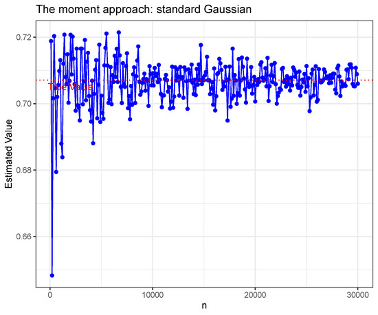
Figure 1. Standard Gaussian.

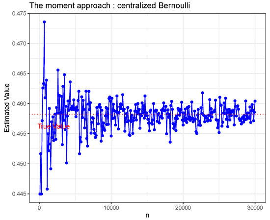
Figure 2. Centralized Bernoulli.

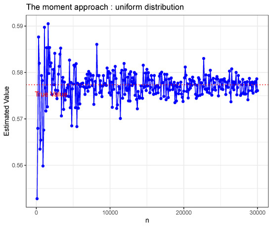
Figure 3. Uniform on $[-1,1]$.

For centralized negative binomial, and centralized Poisson ($\lambda =1$) variable X, ${\parallel X\parallel }_{{\phi }_1}=2.460938,0.7357589,$ respectively. The Figure 4 and Figure 5 show the estimated value from different n under estimate method (8) for the four distributions mentioned above.

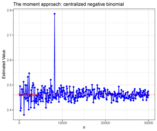
Figure 4. Centralized negative binomial.

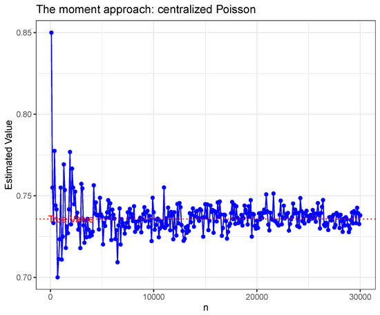
Figure 5. Centralized Poisson.

The five figures mentioned above show litter bias between the estimated norm and true norm. It is worthy to note that the norm estimator for centralized negative binomial case has a peak point. This is caused by sub-exponential distributions having relatively heavy tails, and hence the norm estimation may not robust as that in sub-Gaussian under relatively small sample sizes.

Moreover, sub-Gaussian and sub-exponential parameter is extensible for random vectors with values in a normed space $(\mathcal{X},\parallel ·\parallel )$, we define norm-sub-Gaussian parameter and norm-sub-exponential parameter: The norm-sub-Gaussian parameter:

${∥\mathit{X}∥}_{{\phi }_2}={sup}_{k\ge 1}{(k!)}^{-1/\left(2k\right)}{\left({\mathrm{E}\parallel \mathit{X}\parallel }^{2k}\right)}^{1/\left(2k\right)}$;

the norm-sub-exponential parameter:

${∥\mathit{X}∥}_{{\phi }_1}={sup}_{k\ge 1}{(k!)}^{-1/k}{\left({\mathrm{E}\parallel \mathit{X}\parallel }^k\right)}^{1/k}.$

We denote $\mathit{X}\sim {\mathrm{nsubG}}_{{\phi }_1}\left({\sigma }^2\right)$ and $\mathit{X}\sim {\mathrm{nsubG}}_{{\phi }_2}\left({\sigma }^2\right)$ for ${\sigma }^2={∥\mathit{X}∥}_{{\phi }_2}\mathrm{and}{∥\mathit{X}∥}_{{\phi }_1}$, respectively.

3. Statistical Applications of Sub-Weibull Concentrations

3.1. Negative Binomial Regressions with Heavy-Tail Covariates

In statistical regression analysis, the responses ${\left\{Y_i\right\}}_{i=1}^n$ in linear regressions are assume to be continuous Gaussian variables. However, the category in classification or grouping may be infinite with index by the non-negative integers. The categorical variables is treated as countable responses for distinction categories or groups; sometimes it can be infinite. In practice, random count responses include the number of patients, the bacterium in the unit region, or stars in the sky and so on. The responses ${\left\{Y_i\right\}}_{i=1}^n$ with covariates ${\left\{X_i\right\}}_{i=1}^n$ belongs to generalized linear regressions. We consider i.i.d. random variables ${\left\{(X_i,Y_i)\right\}}_{i=1}^n\sim (X,Y)\in {\mathbb{R}}^p\times \mathbb{N}$. By the methods of the maximum likelihood or the M-estimation, the estimator ${\widehat{\beta }}_n$ is given by

$${\widehat{\beta }}_n:=\underset{\beta \in {\mathbb{R}}^p}{argmin}\frac{1}{n}\sum _{i=1}^n\ell (X_i^{\top }\beta ,Y_i),$$

(9)

where the loss function $\ell (·,·)$ is convex and twice differentiable in the first argument.

In high-dimensional regressions, the dimension $\mathbf{\beta }$ may be growing with sample size n. When ${\left\{Y_i\right\}}_{i=1}^n$ belongs to the exponential family, [18] studied the asymptotic behavior of ${\widehat{\beta }}_n$ in the generalized linear models (GLMs) as $p_n:=\dim \left(X\right)$ is increasing. In our study, we focus on the case that the covariates is $subW\left(\theta \right)$ heavy-tailed for $\theta <1$.

The target vector ${\beta }^{\ast }:=\underset{\beta \in {\mathbb{R}}^p}{argmin}\mathrm{E}\ell \left(X^T\beta ,Y\right)$ is assumed to be the loss under the population expectation, comparing to (9). Let $\dot{\ell }(u,y):={\left.\frac{\partial }{\partial t}\ell (t,y)\right|}_{t=u}$, $\ddot{\ell }(u,y):={\left.\frac{\partial }{\partial t}\dot{\ell }(t,y)\right|}_{t=u}$ and $C(u,y):={sup}_{|s-t|\le u}\frac{\ddot{\ell }(s,y)}{\ddot{\ell }(t,y)}$. Finally, define the score function and Hessian matrix of the empirical loss function are ${\widehat{\mathcal{Z}}}_n\left(\beta \right):=\frac{1}{n}{\sum }_{i=1}^n\dot{\ell }(X_i^T\beta ,Y_i)X_i$ and ${\widehat{\mathcal{Q}}}_n\left(\beta \right):=\frac{1}{n}{\sum }_{i=1}^n\ddot{\ell }(X_i^T\beta ,Y_i)X_i{X}_i^T$, respectively. The population version of Hessian matrix is $\mathcal{Q}\left(\beta \right):=\mathrm{E}\left[\ddot{\ell }(X^T\beta ,Y)X{X}^T\right]$. The following so-called determining inequalities guarantee the ${\ell }_2$-error for the estimator obtained from the smooth M-estimator defined as (9).

Lemma 4

(Corollary 3.1 in [19]). Let ${\delta }_n\left(\beta \right):=\frac{3}{2}{\parallel {\left[{\widehat{\mathcal{Q}}}_n\left(\beta \right)\right]}^{-1}{\widehat{\mathcal{Z}}}_n\left(\beta \right)\parallel }_2$ for $\beta \in {\mathbb{R}}^p$. If $\ell (·,·)$ is a twice differentiable function that is convex in the first argument and for some ${\beta }^{\ast }\in {\mathbb{R}}^p$: ${max}_{1\le i\le n}C\left({∥X_i∥}_2{\delta }_n\left({\beta }^{\ast }\right),Y_i\right)\le \frac{4}{3}$. Then there exists a vector ${\widehat{\beta }}_n\in {\mathbb{R}}^p$ satisfying ${\widehat{\mathcal{Z}}}_n\left({\widehat{\beta }}_n\right)=0$ as the estimating equation of (9),

$$\frac{1}{2}{\delta }_n\left({\beta }^{\ast }\right)\le {\parallel {\widehat{\beta }}_n-{\beta }^{\ast }\parallel }_2\le {\delta }_n\left({\beta }^{\ast }\right).$$

Applications of Lemma 4 in regression analysis is of special interest when X is heavy tailed, i.e., the sub-Weibull index $\theta <1$. For the negative binomial regression (NBR) with the known dispersion parameter $k>0$, the loss function is

$$\ell (u,y)=-yu+(y+k)log(k+e^u).$$

(10)

Thus we have $\dot{\ell }(u,y)=-\frac{k(y-e^u)}{k+e^u},\ddot{\ell }(u,y)=\frac{k(y+k)e^u}{{(k+e^u)}^2}$, see [20] for details.

Further computation gives $C(u,y)={sup}_{|s-t|\le u}\frac{e^s{(k+e^t)}^2}{{(k+e^s)}^2{e}^t}$ and it implies that $C(u,y)\le e^{3u}.$ Therefore, condition ${max}_{1\le i\le n}C\left({∥X_i∥}_2{\delta }_n\left({\beta }^{\ast }\right),Y_i\right)\le \frac{4}{3}$ in Lemma 4 leads to

${max}_{1\le i\le n}{∥X_i∥}_2{\delta }_n\left({\beta }^{\ast }\right)\le \frac{log(4/3)}{3}.$

This condition need the assumption of the design space for ${max}_{1\le i\le n}{∥X_i∥}_2$.

In NBR with loss (10), one has

${\widehat{\mathcal{Q}}}_n\left({\beta }^{\ast }\right):=\frac{1}{n}{\displaystyle \sum _{i=1}^n}\frac{(Y_i+k)k{e}^{X_i^{\top }{\beta }^{\ast }}{X}_i{X}_i^{\top }}{{(k+e^{X_i^{\top }{\beta }^{\ast }})}^2}$ and ${\widehat{\mathcal{Z}}}_n\left({\beta }^{\ast }\right):=\frac{-1}{n}\sum _{i=1}^n\frac{k(Y_i-e^{X_i^{\top }{\beta }^{\ast }})X_i}{k+e^{X_i^{\top }{\beta }^{\ast }}}$.

To guarantee that ${\widehat{\beta }}_n$ approximates ${\beta }^{\ast }$ well, some regularity conditions are required.

•

(C.1): For $M_Y,M_X>0$, assume $\underset{1\le i\le n}{max}\parallel Y_i{\parallel }_{{\psi }_1}\le M_Y$ and the heavy-tailed covariates $\left\{X_{ik}\right\}$ are uniformly sub-Weibull with $\underset{1\le i\le n,1\le k\le p}{max}{∥X_{ik}∥}_{{\psi }_{\theta }}\le M_X$ for $0<\theta <1$.

•

(C.2): The vector $X_i$ is sparse or bounded. Let ${\mathcal{F}}_Y:=\{\underset{1\le i\le n}{max}\mathrm{E}{Y}_i=\underset{1\le i\le n}{max}{e}^{X_i^{\top }{\beta }^{\ast }}\le B,\underset{1\le i\le n}{max}\parallel {\mathit{X}}_i{\parallel }_2\le I_n\}$ with a slowly increasing function $I_n$, we have $\mathrm{P}\left\{{\mathcal{F}}_Y^c\right\}={\epsilon }_n\to 0$.

In addition, to bound $\underset{1\le i\le n,1\le i\le k}{max}|X_{ik}^{}|$, the sub-Weibull concentration determines:

$$\mathrm{P}\left(\underset{1\le i\le n,1\le i\le k}{max}|X_{ik}|>t\right)\le np\mathrm{P}(|X_{11}|>t)\le 2np{e}^{-{(t/{∥X_{11}∥}_{{\psi }_{\theta }})}^{\theta }}\le \delta \Rightarrow t=M_X{log}^{1/\theta }\left(\frac{2np}{\delta }\right),$$

by using Corollary 3. Hence, we define the event for the maximum designs:

$${\mathcal{F}}_{max}=\left\{\underset{1\le i\le n,1\le k\le p}{max}|X_{ik}|\le M_X{log}^{1/\theta }\left(\frac{2np}{\delta }\right)\right\}\cap {\mathcal{F}}_Y.$$

To make sure that the optimization in (9) has a unique solution, we also require the minimal eigenvalue condition.

•

(C.3): Suppose that $b^{\top }\mathrm{E}\left({\widehat{\mathcal{Q}}}_n\left(\beta \right)\right)b\ge C_{min}$ is satisfied for all $b\in S^{p-1}$.

In the proof, to ensure that the random Hessian function has a non-singular eigenvalue, we define the event

$${\mathcal{F}}_1=\left\{\underset{k,j}{max}\left|\frac{1}{n}\sum _{i=1}^n\left[\frac{Y_{i}k{e}^{X_i^{\top }{\beta }^{\ast }}{X}_{ik}{X}_{ij}}{{(k+e^{X_i^{\top }{\beta }^{\ast }})}^2}-\mathrm{E}\left(\frac{Y_{i}k{e}^{X_i^{\top }{\beta }^{\ast }}{X}_{ik}{X}_{ij}}{{(k+e^{X_i^{\top }{\beta }^{\ast }})}^2}\right)\right]\right|\le \frac{C_{min}}{4}\right\}$$

$${\mathcal{F}}_2=\left\{\underset{k,j}{max}\left|\frac{1}{n}\sum _{i=1}^n\left[\frac{k{e}^{X_i^{\top }{\beta }^{\ast }}{X}_{ik}{X}_{ij}}{{(k+e^{X_i^{\top }{\beta }^{\ast }})}^2}-\mathrm{E}\left(\frac{k{e}^{X_i^{\top }{\beta }^{\ast }}{X}_{ik}{X}_{ij}}{{(k+e^{X_i^{\top }{\beta }^{\ast }})}^2}\right)\right]\right|\le \frac{C_{min}}{4}\right\}.$$

Theorem 3

(Upper bound for ${\ell }_2$-error). In the NBR with loss (10) and $(C.1-C.3)$, let

$$M_{BX}=M_X+\frac{B}{log2},R_n:=\frac{6M_{BX}{M}_X}{C_{min}}\left[\sqrt{\frac{2p}{n}log\left(\frac{2p}{\delta }\right)}+\frac{1}{n}\sqrt{plog\left(\frac{2p}{\delta }\right)}\right]{log}^{1/\theta }\left(\frac{2np}{\delta }\right),$$

and $\mathit{b}:=(k/n)M_X^2{(1,\dots ,1)}^{\top }\in {\mathbb{R}}^n$. Under the event ${\mathcal{F}}_1\cap {\mathcal{F}}_2\cap {\mathcal{F}}_{max}$, for any $0<\delta <1$, if the sample size n satisfies

$$R_n{I}_n\le \frac{log(4/3)}{3},$$

(11)

Let $c_n:=e^{-\frac{1}{4}(\frac{n{t}^2}{2M_X^4{log}^{4/\theta }\left(\frac{2np}{\delta }\right)M_{BX}^2}\wedge \frac{nt}{M_X^2{log}^{2/\theta }\left(\frac{2np}{\delta }\right)M_{BX}})}+e^{-(\frac{t^{\theta /2}}{{\left[4eC(\theta /2){∥\mathit{b}∥}_2{L}_n(\theta /2,\mathit{b})\right]}^{\theta /2}}\wedge \frac{t^2}{16e^2{C}^2(\theta /2){∥\mathit{b}∥}_2^2})}$ with $t=C_{min}/4$, then

$$\mathrm{P}(\parallel {\widehat{\beta }}_n-{\beta }^{\ast }{\parallel }_2\le R_n)\ge 1-2p^2{c}_n-\delta -{\epsilon }_n.$$

A few comment is made on this theorem. First, in order to get $\parallel {\widehat{\beta }}_n-{\beta }^{\ast }{\parallel }_2\stackrel{p}{\to }0$, we need $p=o\left(n\right)$ under sample size restriction (11) with $I_n=o({log}^{-1/\theta }\left(np\right)·[n^{-1}plogp{]}^{-1/2})$. Second, note that the ${\epsilon }_n$ in provability $1-2p^2{c}_n-\delta -{\epsilon }_n$ depends on the models size and the fluctuation of the design by the event ${\mathcal{F}}_{max}$.

3.2. Non-Asymptotic Bai-Yin’s Theorem

In statistical machine learning, exponential decay tail probability is crucial to evaluate the finite-sample performance. Unlike Bai-Yin’s law with the fourth-moment condition that leads to polynomial decay tail probability, under sub-Weibull conditions of data, we provide a exponential decay tail probability on the extreme eigenvalues of a $n\times p$ random matrix.

Let $\mathbf{A}={\mathbf{A}}_{n,p}$ be an $n\times p$ random matrix whose entries are independent copies of a r.v. with zero mean, unit variance, and finite fourth moment. Suppose that the dimensions n and p both grow to infinity while the aspect ratio $p/n$ converges to a constant in $[0,1]$. Then Bai-Yin’s law [21] asserted that the standardized extreme eigenvalues satisfying

$\frac{1}{\sqrt{n}}{\lambda }_{min}\left(\mathbf{A}\right)=1-\sqrt{\frac{p}{n}}+o\left(\sqrt{\frac{p}{n}}\right),\frac{1}{\sqrt{n}}{\lambda }_{max}\left(\mathbf{A}\right)=1+\sqrt{\frac{p}{n}}+o\left(\sqrt{\frac{p}{n}}\right)\mathrm{a}.\mathrm{s}..$

Next we introduce a special counting measure for measuring the complexity of a certain set in some space. The ${\mathcal{N}}_{\epsilon }$ is called an ε-net of K in ${\mathbb{R}}^n$ if K can be covered by balls with centers in K and radii $\epsilon$ (under Euclidean distance). The covering number$\mathcal{N}(K,\epsilon )$ is defined by the smallest number of closed balls with centers in K and radii $\epsilon$ whose union covers K.

For purposes of studying random matrices, we need to extend the definition of sub-Weibull r.v. to sub-Weibull random vectors. The n-dimensional unit Euclidean sphere $S^{n-1}$, is denoted by $S^{n-1}=\{\mathit{x}\in {\mathbb{R}}^n:{∥\mathit{x}∥}_2=1\}.$ We say that a random vector $\mathit{X}$ in ${\mathbb{R}}^n$ is sub-Weibull if the one-dimensional marginals $⟨\mathit{X},\mathit{a}⟩$ are sub-Weibull r.v.s for all $\mathit{a}\in {\mathbb{R}}^n$. The sub-Weibull norm of a random vector $\mathit{X}$ is defined as ${\parallel \mathit{X}\parallel }_{{\psi }_{\theta }}:={sup}_{\mathit{a}\in S^{n-1}}{\parallel ⟨\mathit{X},\mathit{a}⟩\parallel }_{{\psi }_{\theta }}.$ Similarly, define the spectral norm for any $p\times p$ matrix $\mathbf{B}$ as $\parallel \mathbf{B}\parallel ={max}_{{||\mathsf{x}||}_2=1}\parallel \mathbf{B}\mathit{x}{\parallel }_2={sup}_{\mathit{x}\in S^{p-1}}|⟨\mathbf{B}\mathit{x},\mathit{x}⟩|$. Spectral norm has many good properties, see [1] for details.

Furthermore, for simplicity, we assume that the rows in random matrices are isotropic random vectors. A random vector $\mathit{Y}$ in ${\mathbb{R}}^n$ is called isotropic if $\mathrm{Var}\left(\mathit{Y}\right)={\mathbf{I}}_p.$ Equivalently, $\mathit{Y}$ is isotropic if $\mathrm{E}\left[{⟨\mathit{Y},\mathit{a}⟩}^2\right]={\parallel \mathit{a}\parallel }_2^2\mathrm{for}\mathrm{all}\mathit{a}\in {\mathbb{R}}^n.$ In the non-asymptotic regime, Theorem 4.6.1 in [1] study the upper and lower bounds of maximum (minimum) eigenvalues of random matrices with independent sub-Gaussian entries which are sampled from high-dimensional distributions. As an extension of Theorem 4.6.1 in [1], the following result is a non-asymptotic versions of Bai-Yin’s law for sub-Weibull entries, which is useful to estimate covariance matrices from heavy-tailed data [$subW\left(\theta \right)$, $\theta <1$].

Theorem 4 (Non-asymptotic Bai-Yin’s law).

Let $\mathbf{A}$ be an $n\times p$ matrix whose rows ${\mathit{A}}_i$ are independent isotropic sub-Weibull random vectors in ${\mathbb{R}}^p$ with covariance matrix ${\mathbf{I}}_p$ and ${max}_{1\le i\le n}{\parallel {\mathbf{A}}_i\parallel }_{{\psi }_{\theta }}\le K$. Then for every $s\ge 0$, we have

$$\mathrm{P}\left\{\parallel \frac{1}{n}{\mathbf{A}}^{\top }\mathbf{A}-{\mathbf{I}}_p\parallel \le H(cp+s^2,n;\theta )\right\}\ge 1-2e^{-s^2},$$

where

$$H(t,n;\theta ):=2eKC(\theta /2)K_{\theta /2}[1+{(\left[{\left(e\theta /2\right)}^{\theta /2}\right]log2)}^{-\theta /2})\left[\sqrt{\frac{t}{n}}+\left\{\begin{array}{cc}A(\theta /2)\frac{{\left({\gamma }^{2}t\right)}^{2/\theta }}{n},\hfill & \theta \le 2\hfill \\ B(\theta /2)\frac{{\left({\gamma }^{2}t\right)}^{2/\theta }}{n^{1/\theta }},\hfill & \theta >2\hfill \end{array}\right.\right],$$

where $K_{\alpha }:=2^{1/\alpha }$ if $\alpha \in (0,1)$ and $K_{\alpha }=1$ if $\alpha \ge 1$; $A(\theta /2)$, $B(\theta /2)$ and $C(\theta /2)$ defined in Theorem 1a.

Moreover, the concentration inequality for extreme eigenvalues hold for $c\ge nlog9/p$

$$\mathrm{P}\left\{\sqrt{1-H^2(cp+s^2,n;\theta )}\le \frac{{\lambda }_{min}\left(\mathbf{A}\right)}{\sqrt{n}}\le \frac{{\lambda }_{max}\left(\mathbf{A}\right)}{\sqrt{n}}\le \sqrt{1+H^2(cp+s^2,n;\theta )}\right\}\ge 1-2e^{-s^2}.$$

(12)

3.3. General Log-Truncated Z-Estimators and sub-Weibull Type Robust Estimators

Motivated from log-truncated loss in [22,23], we study the almost surely continuous and non-decreasing function ${\phi }^c:\mathbb{R}\to \mathbb{R}$ for truncating the original score function

$$\begin{array}{c}\hfill -log\left[1-x+c(|x|)\right]\le {\phi }^c\left(x\right)\le log\left[1+x+c(|x|)\right],\forall x\in \mathbb{R}\end{array}$$

(13)

where $c(|x|)>0$ is a high-order function [23] of $|x|$ which is to be specified. For example, a plausible choose for ${\phi }^c\left(x\right)$ in (13) should have following form

$$\begin{array}{cc}\hfill {\phi }^c\left(x\right)& =log\left[1+x+c(|x|)\right]1(x\ge 0)-log\left[1-x+c(|x|)\right]1(x\le 0)\hfill \\ \hfill & =\mathrm{sign}\left(x\right)log(1+|x|+c(|x|\left)\right).\hfill \end{array}$$

(14)

For (14), we get ${\phi }^c\left(x\right)\approx x$ for sufficiently smaller x and ${\phi }^c\left(x\right)\ll x$ for larger x. Under (13), now we show that $c(|x|)$ must obey a key inequality. For all $x\in \mathbb{R}$, it suffices to verify $-log[1-x+\mathrm{c}(|x|\left)\right]\le log[1+x+\mathrm{c}(|x|\left)\right]$, which is equivalent to check $log\left[\left(1+\mathrm{c}(|x|)+x\right)\left(1+\mathrm{c}(|x|)-x\right)\right]\ge 0$, namely ${\left(1+\mathrm{c}(|x|)\right)}^2-x^2\ge 1\iff \mathrm{c}(|x|)\ge \sqrt{1+x^2}-1.$

For independent r.v.s ${\left\{X_i\right\}}_{i=1}^n$, using the score function (14), we define the score function of data

${\widehat{Z}}_{{\alpha }_n}\left(\theta \right)=\frac{1}{n{\alpha }_n}{\sum }_{i=1}^n{\phi }^c\left[{\alpha }_n\left(X_i-\theta \right)\right]$ for any $\theta \in \mathbb{R}$.

Then the influence of the heavy-tailed outliers is weaken by ${\phi }^c\left[{\alpha }_n\left(X_i-\theta \right)\right]$ by choosing an optimal ${\alpha }_n$. We aim to estimate the average mean: ${\mu }_n:=\frac{1}{n}{\sum }_{i=1}^n\mathrm{E}{X}_i$ for non-i.i.d. samples ${\left\{X_i\right\}}_{i=1}^n$. Define the Z-estimator ${\widehat{\theta }}_{{\alpha }_n}$ as

$$\begin{array}{c}\hfill {\widehat{\theta }}_{{\alpha }_n}\in \{\theta \in \mathbb{R}:{\widehat{Z}}_{{\alpha }_n}\left(\theta \right)=0\},\end{array}$$

(15)

where ${\alpha }_n$ is the tuning parameter (will be determined later).

To guarantee consistency for log-truncated Z-estimators (15), we require following assumptions of $c(·)$.

•

(C.1): For a constant $c_2>1$, the $c\left(x\right)$ satisfies weak triangle inequality and scaling property,

$$(\mathrm{C}.1.1):c(x+y)\le c_2[c\left(x\right)+c\left(y\right)],(\mathrm{C}.1.2):c\left(tx\right)\le f\left(t\right)c\left(x\right)$$

for $f\left(t\right)$ satisfies

(C.1.3): $f\left(t\right)$ and $f\left(t\right)/|t|$ are non-constant increasing functions and $\underset{t\to 0}{lim}f\left(t\right)/|t|=0$.

Remark 6.

Note that $|x|\ge \sqrt{1+x^2}-1$ and we could put $c(|x|)=|x|$. However, $c(|x|)=|x|$ does not satisfy (C.1.3) since $f\left(t\right)=|t|$ and $f\left(t\right)/|t|$ are constant functions of t.

In the following theorem, we establish the finite sample confidence interval and the convergence rate of the estimator ${\widehat{\theta }}_{{\alpha }_n}$.

Theorem 5.

Let ${\left\{X_i\right\}}_{i=1}^n$ be independent samples drawn from an unknown probability distribution ${\left\{P_i\right\}}_{i=1}^n$ on $\mathbb{R}$. Consider the estimator ${\widehat{\theta }}_{{\alpha }_n}$ defined as (15) with (C.1), ${\alpha }_n\to 0$ and $\frac{1}{n}{\sum }_{i=1}^n\mathrm{E}\left[c(X_i-\theta )\right]=O\left(1\right)$. Let $B_n^{+}\left(\theta \right)={\mu }_n-\theta +\frac{1}{n{\alpha }_n}{\sum }_{i=1}^n\mathrm{E}\left[c\left({\alpha }_n(X_i-\theta )\right)\right]+\frac{log\left({\delta }^{-1}\right)}{n{\alpha }_n}$ and $B_n^{-}\left(\theta \right)={\mu }_n-\theta -\frac{1}{n{\alpha }_n}{\sum }_{i=1}^n\mathrm{E}\left[c\left({\alpha }_n(X_i-\theta )\right)\right]-\frac{log\left({\delta }^{-1}\right)}{n{\alpha }_n}$. Let ${\theta }_{+}$ be the smallest solution of the equation $B_n^{+}\left(\theta \right)=0$ and ${\theta }_{-}$ be the largest solution of $B_n^{-}\left(\theta \right)=0$.

(a). We have with the $(1-2\delta )$-confidence intervals

$$\mathrm{P}(B_n^{-}\left(\theta \right)<{\widehat{Z}}_{{\alpha }_n}\left(\theta \right)<B_n^{+}\left(\theta \right))\ge 1-2\delta ,\mathrm{P}({\theta }_{-}\le {\widehat{\theta }}_{{\alpha }_n}\le {\theta }_{+})\ge 1-2\delta ,$$

for any $\delta \in (0,1/2)$ satisfies the sample condition:

$$\begin{array}{c}\hfill \frac{1}{n{\alpha }_n}\sum _{i=1}^n\mathrm{E}\left[c\left({\alpha }_n{X}_i-{\alpha }_n[{\mu }_n\pm d_n\left(c\right)]\right)\right]+\frac{log\left({\delta }^{-1}\right)}{n{\alpha }_n}<d_n\left(c\right),\end{array}$$

(16)

where $d_n\left(c\right)$ is a constant such that $B_n^{\pm }({\mu }_n\pm d_n\left(c\right))<0$.

(b). Moreover, picking ${\alpha }_n\ge f^{-1}\left(\frac{log\left({\delta }^{-1}\right)}{c_2{\sum }_{i=1}^n\mathrm{E}\left[c\left(X_i-{\mu }_n\right)\right]}\right)$, one has

$$\begin{array}{c}\hfill \mathrm{P}\left(|{\widehat{\theta }}_{{\alpha }_n}-{\mu }_n|\le \left|g_{{\alpha }_n}^{-1}\left\{-\frac{2log\left({\delta }^{-1}\right)}{n{\alpha }_n}\right\}\right|\right)\ge 1-2\delta ,\mathrm{with}{g}_{{\alpha }_n}\left(t\right):=t+\frac{c_2}{{\alpha }_n}c\left({\alpha }_{n}t\right).\end{array}$$

(17)

The (17) in Theorem 5 is a fundamental extension of Lemma 2.1 (see Theorem 16 in [24]) with $c\left(x\right)=x^2/2$ from i.i.d. sample to independent sample. Let $c\left(x\right)={|x|}^{\beta }/\beta$, for i.i.d. sample, Theorem 5 implies Lemmas 2.3, 2.4 and Theorem 2.1 in [22]. The ${\alpha }_n\ge f^{-1}\left(\frac{log\left({\delta }^{-1}\right)}{c_2{\sum }_{i=1}^n\mathrm{E}\left[c\left(X_i-{\mu }_n\right)\right]}\right)$ in Theorem 5(b) gives a theoretical guarantee for choosing the tuning parameter ${\alpha }_n$.

Proposition 7

(Theorem 2.1 in [22]). Let ${\left\{X_i\right\}}_{i=1}^n$ be a sequence of i.i.d. samples drawn from an unknown probability distribution on $\mathbb{R}$. We assume $\mathrm{E}{\left|X_1\right|}^{\beta }<\infty$ for a certain $\beta \in (1,2]$ and denote $\mu =\mathrm{E}\left[X_1\right],v_{\beta }=\mathrm{E}{\left|X_1-\mu \right|}^{\beta }$. Given any $ϵ\in (0,1/2)$ and positive integer $n\ge {\left(\frac{2v_{\beta }+1}{\beta }\right)}^{\frac{\beta }{\beta -1}}\frac{2\beta log\left({ϵ}^{-1}\right)}{v_{\beta }}$, let ${\alpha }_n=\frac{1}{2}{\left(\frac{2\beta log\left({ϵ}^{-1}\right)}{n{v}_{\beta }}\right)}^{\frac{1}{\beta }}.$ Then, with probability at least $1-2ϵ$,

$$\begin{array}{c}\hfill |{\widehat{\theta }}_{{\alpha }_n}-\mu |\le 2{\left(\frac{2\beta log\left({ϵ}^{-1}\right)}{n}\right)}^{\frac{\beta -1}{\beta }}{v}_{\beta }^{\frac{1}{\beta }}{\left[\beta -{\left(\frac{2\beta log\left({ϵ}^{-1}\right)}{n{v}_{\beta }}\right)}^{\frac{\beta -1}{\beta }}\right]}^{-1}=O\left(n^{-\frac{\beta -1}{\beta }}\right).\end{array}$$

(18)

Comparing to the convergence rate in (18), put $O\left(n^{-\frac{\beta -1}{\beta }}\right)=O\left(n^{-1/\theta }\right)$ for $\theta >2$. It implies

$${\beta }^{-1}+{\theta }^{-1}=1,(\theta \ge 2\mathrm{or}0<\beta \le 2).$$

For example, let us deal with the Pareto distribution $\mathrm{Pareto}(\alpha ,k)$ with shape parameter $\alpha >0$ and scale parameter $k>0$, and the density function is $f\left(x\right)=\frac{\alpha k^{\alpha }}{x^{\alpha +1}}·1_{\{x\in [k,\infty \left)\right\}}$. For $\alpha \le 2$, $\mathrm{Pareto}(\alpha ,k)$ has infinite variance, and it does not belong to the sub-Weibull distribution, so do the sample mean of i.i.d. Pareto distributed data. Proposition 7 shows that the estimator error for robust mean estimator enjoys sub-Weibull concentration as presented in Proposition 3, without finite sub-Weibull norm assumption of data. With the Weibull-tailed behavior, it motivates us to define general sub-Weibull estimators having the non-parametric convergence rate $O\left(n^{-1/\theta }\right)$ in Proposition 3 for $\theta >2$, even if the data do not have finite sub-Weibull norm.

Definition 5

(Sub-Weibull estimators). An estimator $\widehat{\mu }:=\widehat{\mu }(X_1,\cdots ,X_n)$ based on i.i.d. samples ${\left\{X_i\right\}}_{i=1}^n$ from an unknown probability distribution P with mean ${\mu }_P$, is called $(A,B,C)$-$subW\left(\theta \right)$ if

$$\forall t\in (0,A),\mathrm{P}(|\widehat{\mu }-{\mu }_P|\le B{\left(t/n\right)}^{1/\theta })\ge 1-C{e}^{-t}.$$

For example, in Proposition 7, ${\widehat{\theta }}_{{\alpha }_n}$ is $(\infty ,B,1)$-$subW\left(\frac{\beta }{\beta -1}\right)$ with $B\sim 2{\left(2\beta log\left({ϵ}^{-1}\right)\right)}^{\frac{\beta -1}{\beta }}{v}_{\beta }^{\frac{1}{\beta }}$ in Definition 5. When $\theta =2$, [25] defined sub-Gaussian estimators (includes Median of means and Catoni’s estimators) for certain heavy-tailed distributions and discussed the nonexistence of sub-Gaussian mean estimators under $\beta$-moment condition for the data ($\beta \in (1,2)$).

4. Conclusions

Concentration inequalities are far-reaching useful in high-dimensional statistical inferences and machine learnings. They can facilitate various explicit non-asymptotic confidence intervals as a function of the sample size and model dimension.

Future research includes sharper version of Theorem 2 that is crucial to construct non-asymptotic and data-driven confidence intervals for the sub-Weibull sample mean. Although we have obtained sharper upper bounds for sub-Weibull concentrations, the lower bounds on tail probabilities are also important in some statistical applications [26]. Developing non-asymptotic and sharp lower tail bounds of Weibull r.v.s is left for further study. For negative binomial concentration inequalities in Corollary 2, it is of interesting to study concentration inequalities of COM-negative binomial distributions (see [27]).

Appendix A.1

Proof of Corollary 1.

${\varphi }_{{|X|}^{\theta }}\left(t\right)$ is continuous for t a neighborhood of zero, by the definition, $2\ge \mathrm{E}{e}^{(|X|/{\parallel X\parallel }_{{\psi }_{\theta }}{)}^{\theta }}=m_{{|X|}^{\theta }}\left({\parallel X\parallel }_{{\psi }_{\theta }}^{-\theta }\right).$ Since ${|X|}^{\theta }>0$, the MGF $m_{{|X|}^{\theta }}\left(t\right)$ is monotonic increasing. Hence, inverse function $m_{{|X|}^{\theta }}^{-1}\left(t\right)$ exists and ${\parallel X\parallel }_{{\psi }_{\theta }}^{-\theta }=m_{{|X|}^{\theta }}^{-1}\left(2\right).$ So ${\parallel X\parallel }_{{\psi }_{\theta }}={\left(m_{{|X|}^{\theta }}^{-1}\left(2\right)\right)}^{-1/\theta }$. □

Appendix A.2

Proof of Corollary 2.

The first inequality is the direct application of (3) by observing that for any constant $a\in \mathbb{R}$, and r.v. Y with ${\parallel Y\parallel }_{{\psi }_1}<\infty$, ${\parallel aY\parallel }_{{\psi }_1}={|a|\parallel Y\parallel }_{{\psi }_1}$, ${\parallel Y+a\parallel }_{{\psi }_1}\le {\parallel Y\parallel }_{{\psi }_1}+{\parallel a\parallel }_{{\psi }_1}={\parallel Y\parallel }_{{\psi }_1}+|a|/log2$ and ${\parallel X+a\parallel }_{{\psi }_1}^2\le {(\parallel X\parallel }_{{\psi }_1}{+|a|/log2)}^2$. The second inequality is obtained from (3) by considering two rate in $(\frac{t^2}{{\sum }_{i=1}^{n}2{\parallel Y_i\parallel }_{{\psi }_1}^2}\wedge \frac{t}{{max}_{1\le i\le n}{\parallel Y_i\parallel }_{{\psi }_1}})$ separately. For (5), we only need to note that

$$\begin{array}{c}\hfill \parallel Y_i{\parallel }_{{\psi }_1}=inf\{t>0:\mathrm{E}{e}^{Y_i/t}\le 2\}=inf\{t>0:{\left(\frac{1-q_i}{1-q_i{e}^{1/t}}\right)}^{k_i}\le 2\}={\left[log\frac{1-(1-q_i)/\sqrt[k_i]{2}}{q_i}\right]}^{-1}.\end{array}$$

Then the third inequality is obtained by the first inequality and the definition of $a({\mu }_i,k_i)$. □

Appendix A.3

Proof of Corollary  3.

The first and second part of this proposition were shown in Lemma 2.1 of [28]. For the third result, using the bounds of Gamma function [see [29]:

$\sqrt{2\pi }{x}^{x-(1/2)}{e}^{-x}\le \Gamma \left(x\right)\le \left[\sqrt{2\pi }{x}^{x-(1/2)}{e}^{-x}\right]·e^{1/\left(12x\right)},(x>0),$

it gives

$$\begin{array}{cc}\hfill {(\mathrm{E}|X{|}^k)}^{1/k}& \le {\left\{2{\parallel X\parallel }_{{\phi }_{\theta }}^k\left(\frac{k}{\theta }\right)\left[\sqrt{2\pi }{\left(k/\theta \right)}^{\frac{k}{\theta }-\frac{1}{2}}{e}^{-\frac{11k}{12\theta }}\right]\right\}}^{1/k}={\left(\frac{2\sqrt{2\pi }}{\theta }\right)}^{1/k}{\left\{{\left(\frac{k}{\theta }\right)}^{\frac{k}{\theta }+\frac{1}{2}}{e}^{-\frac{11k}{12\theta }}\right\}}^{1/k}{\parallel X\parallel }_{{\phi }_{\theta }}\hfill \\ \hfill & ={\left(\frac{2\sqrt{2\pi }}{\theta }\right)}^{1/k}{\left(k/\theta \right)}^{\frac{1}{\theta }+\frac{1}{2k}}{e}^{-\frac{11}{12\theta }}{\parallel X\parallel }_{{\phi }_{\theta }}\le C_{\theta }{\left(\theta e^{11/12}\right)}^{-1/\theta }{\parallel X\parallel }_{{\phi }_{\theta }}{k}^{1/\theta }.\hfill \end{array}$$

□

Appendix A.4

Proof of Corollary 4.

By the definition of ${\psi }_{\theta }$-norm, $\mathrm{E}exp\{|X/{\parallel X\parallel }_{{\psi }_{\theta }}{|}^{\theta }\}\le 2$. Then $\mathrm{E}exp\{||X{|}^r/{\parallel X\parallel }_{{\psi }_{\theta }}^r{|}^{\theta /r}\}\le 2.$ The result ${|X|}^r\sim subW(\theta /r)$ follows by the definition of ${\psi }_{\theta }$-norm again. Moreover,

$$\begin{array}{cc}\hfill {\parallel X\parallel }_{{\psi }_{\theta }}:& ={inf\{C\in (0,\infty ):\mathrm{E}[exp(|X|}^{\theta }/C^{\theta }\left)\right]\le 2\}\hfill \\ \hfill & =[inf\{C^r\in {(0,\infty ):\mathrm{E}[exp\{||X|}^r/C^r{|}^{\theta /r}\left\}\right]\le {2\left\}\right]}^{1/r}={∥{|X|}^r∥}_{{\psi }_{\theta /r}}^{1/r},\hfill \end{array}$$

which verifies (6). If $X\sim subW\left(r\theta \right)$, then $\mathrm{E}exp\{|X^r/{\parallel X\parallel }_{{\psi }_{r\theta }}^r{|}^{\theta }\}=\mathrm{E}exp\{|X/{\parallel X\parallel }_{{\psi }_{r\theta }}{|}^{r\theta }\}\le 2$, which means that $X^r\sim subW\left(\theta \right)$ with

$$\begin{array}{cc}\hfill {\parallel X\parallel }_{{\psi }_{r\theta }}:& ={inf\{C\in (0,\infty ):\mathrm{E}[exp(|X|}^{r\theta }/C^{r\theta }\left)\right]\le 2\}\hfill \\ \hfill & =[inf\{C^r\in {(0,\infty ):\mathrm{E}[exp\{||X|}^r/C^r{|}^{\theta }\left\}\right]\le {2\left\}\right]}^{1/r}={∥{|X|}^r∥}_{{\psi }_{\theta }}^{1/r}.\hfill \end{array}$$

□

Appendix A.5

Proof of Corollary 5.

Set $\Delta :={sup}_{p\ge 2}\frac{{\parallel X\parallel }_p}{\sqrt{p}+L{p}^{1/\theta }}$ so that ${\parallel X\parallel }_p\le \Delta \sqrt{p}+L\Delta p^{1/\theta }$ holds for all $p\ge 2$. By Markov’s inequality for t-th moment $(t\ge 2)$, we have

$$\begin{array}{cc}\hfill \mathrm{P}\left(|X|\ge e\Delta \sqrt{t}+eL\Delta t^{1/\theta }\right)& \le {\left(\frac{{||X||}_t}{e\Delta [\sqrt{t}+L{t}^{1/\theta }]}\right)}^t\le e^{-t},[\mathrm{By}\mathrm{the}\mathrm{definition}\mathrm{of}\Delta ].\hfill \end{array}$$

So, for any $t\ge 2$,

$$\mathrm{P}\left(|X|\ge e\Delta \sqrt{t}+eL\Delta t^{1/\theta }\right)\le e^{-t}.$$

(A1)

Note the definition of $\Delta$ shows ${\parallel X\parallel }_t\le \Delta \sqrt{t}+L\Delta t^{1/\theta }$ holds for all $t\ge 2$ and assumption ${\parallel X\parallel }_t\le C_1\sqrt{t}+C_2{t}^{1/\theta }$ for all $t\ge 2$. It gives $e\Delta \sqrt{t}+eL\Delta t^{1/\theta }\le e{C}_1\sqrt{t}+e{C}_2{t}^{1/\theta }$. This inequality with (A1) gives

$$\mathrm{P}\left(|X|\ge e{C}_1\sqrt{t}+e{C}_2{t}^{1/\theta }\right)\le 1\{0<t<2\}+e^{-t}\{t\ge 2\},\forall t>0.$$

(A2)

Take $K=k^{2/\theta }{C}_2/\left(k{C}_1\right)$, and define ${\delta }_k:=ke{C}_1$ for a certain constant $k>1$,

$$\begin{array}{cc}\hfill & \mathrm{E}\left[{\Psi }_{\theta ,K}\left(\frac{|X|}{{\delta }_k}\right)\right]={\int }_0^{\infty }\mathrm{P}\left(|X|\ge {\delta }_k{\Psi }_{\theta ,K}^{-1}\left(s\right)\right)ds\hfill \\ \hfill & ={\int }_0^{\infty }\mathrm{P}(|X|\ge ke{C}_1\sqrt{log(1+s)}+ke{C}_{1}K{[log(1+s)]}^{1/\theta })ds\hfill \\ \hfill & ={\int }_0^{\infty }\mathrm{P}(|X|\ge e{C}_1\sqrt{log{(1+s)}^{k^2}}+e{C}_2{[log{(1+s)}^{k^2}]}^{1/\theta })ds\hfill \\ \hfill \mathrm{By}\left(\mathrm{A}2\right)]& \le {\int }_{0<k^{2}log(1+s)<2}ds+{\int }_{k^{2}log(1+s)\ge 2}exp\left\{-k^{2}log(1+s)\right\}ds\hfill \\ \hfill & \le {\int }_0^{e^{2k^{-2}}-1}dt+{\int }_{e^{2k^{-2}}-1}^{\infty }\frac{dt}{{(1+t)}^{k^2}}\hfill \\ \hfill & =e^{2k^{-2}}-1+\frac{{(1+t)}^{1-k^2}}{1-k^2}{\left.\right|}_{e^{2k^{-2}}-1}^{\infty }=e^{2k^{-2}}-1+\frac{e^{2(1-k^2)/k^2}}{k^2-1}\le 1.\hfill \end{array}$$

Therefore, ${\parallel X\parallel }_{{\Psi }_{\theta ,K}}\le \gamma e{C}_1$ with $\gamma$ defined as the smallest solution of the inequality $\{k>1:e^{2k^{-2}}-1+\frac{e^{2(1-k^2)/k^2}}{k^2-1}\le 1\}$. An approximate solution is $\gamma \approx 1.78$. □

Appendix A.6

The main idea in the proof is by the sharper estimates of the GBO norm of the sum of symmetric r.v.s.

Proof of Theorem 1.

(a)

Without loss of generality, we assume $\parallel X_i{\parallel }_{{\psi }_{\theta }}=1$. Define $Y_i:={\left(|X_i{|-(log2)}^{1/\theta }\right)}_{+}$, then it is easy to check that $\mathrm{P}(|X_i|\ge t)\le 2e^{-t^{\theta }}$ implies $\mathrm{P}(Y_i\ge t)\le e^{-t^{\theta }}$. For independent Rademacher r.v. ${\left\{{\epsilon }_i\right\}}_{i=1}^n$, the symmetrization inequality gives ${∥{\sum }_{i=1}^n{w}_i{X}_i∥}_p\le 2{∥{\sum }_{i=1}^n{\epsilon }_i{w}_i{X}_i∥}_p.$ Note that ${\epsilon }_i{X}_i$ is identically distributed as ${\epsilon }_i|X_i|$,

$$\begin{array}{cc}\hfill \parallel \sum _{i=1}^n{w}_i{X}_i{\parallel }_p& \le 2\parallel \sum _{i=1}^n{\epsilon }_i{w}_i|X_i{|\parallel }_p\le 2\parallel \sum _{i=1}^n{\epsilon }_i{w}_i\left(Y_i+{(log2)}^{1/\theta }\right){\parallel }_p\hfill \\ \hfill & \le 2\parallel \sum _{i=1}^n{\epsilon }_i{w}_i{Y}_i{\parallel }_p+2{(log2)}^{1/\theta }\parallel \sum _{i=1}^n{\epsilon }_i{w}_i{\parallel }_p\hfill \\ \hfill [\mathrm{Khinchin}-\mathrm{Kahane}\mathrm{inequality}]& \le 2\parallel \sum _{i=1}^n{\epsilon }_i{w}_i{Y}_i{\parallel }_p+2{(log2)}^{1/\theta }{\left(\frac{p-1}{2-1}\right)}^{1/2}\parallel \sum _{i=1}^n{\epsilon }_i{w}_i{\parallel }_2\hfill \\ \hfill & <2\parallel \sum _{i=1}^n{\epsilon }_i{w}_i{Y}_i{\parallel }_p+2{(log2)}^{1/\theta }\sqrt{p}{\left(\mathrm{E}{\left(\sum _{i=1}^n{\epsilon }_i{w}_i\right)}^2\right)}^{1/2}\hfill \\ \hfill {\left\{{\epsilon }_i\right\}}_{i=1}^n\mathrm{are}\mathrm{independent}]& =2\parallel \sum _{i=1}^n{\epsilon }_i{w}_i{Y}_i{\parallel }_p+2{(log2)}^{1/\theta }\sqrt{p}{\parallel \mathit{w}\parallel }_2.\hfill \end{array}$$

(A3)

From Lemma 2, we are going to handle the first term in (A3) with the sum of symmetric r.v.s. Since $\mathrm{P}(Y_i\ge t)\le e^{-t^{\theta }}$, then

$\parallel {\sum }_{i=1}^n{\epsilon }_i{w}_i{Y}_i{\parallel }_p={\parallel {\sum }_{i=1}^n{w}_i{Z}_i\parallel }_p,Z_i:={\epsilon }_i{Y}_i$

for symmetric independent r.v.s ${\left\{Z_i\right\}}_{i=1}^n$ satisfying $|Z_i|\stackrel{d}{=}{Y}_i$ and $\mathrm{P}(Z_i\ge t)=e^{-t^{\theta }}$ for all $t\ge 0$.

Next, we proceed the proof by checking the moment conditions in Corollary 5.

Case $\theta \le 1$:$N\left(t\right)=t^{\theta }$ is concave for $\theta \le 1$. From Lemmas 2 and 3 (a), for $p\ge 2$,

$$\begin{array}{cc}\hfill & \parallel \sum _{i=1}^n{w}_i{Z}_i{\parallel }_p\le einf\left\{t>0:\sum _{i=1}^{n}log{\varphi }_p\left(e^{-2}\left(\frac{w_i{e}^2}{t}\right)Z_i\right)\le p\right\}\hfill \\ \hfill & \le einf\left\{t>0:\sum _{i=1}^{n}p{M}_{p,Z_i}\left(\frac{w_i{e}^2}{t}\right)\le p\right\}\hfill \\ \hfill & =einf\left\{t>0:\sum _{i=1}^n\left[\left\{{\left(\frac{w_i{e}^2}{t}\right)}^p{\parallel Z_i\parallel }_p^p\right\}\vee \left\{p{\left(\frac{w_i{e}^2}{t}\right)}^2{\parallel Z_i\parallel }_2^2\right\}\right]\le p\right\}\hfill \\ \hfill & \le einf\left\{t>0:\Gamma \left(\frac{p}{\theta }+1\right)\frac{e^{2p}}{t^p}{\parallel \mathit{w}\parallel }_p^p\le 1\right\}+einf\left\{t>0:p\Gamma \left(\frac{2}{\theta }+1\right)\frac{e^4}{t^2}{\parallel \mathit{w}\parallel }_2^2\le 1\right\},\hfill \end{array}$$

where the last inequality we use $\parallel Z_i{\parallel }_p^p={\int }_0^{\infty }p{t}^{p-1}\mathrm{P}(|Z_i|\ge t)dt\le {\int }_0^{\infty }p{t}^{p-1}{e}^{-t^{\theta }}dt=p\Gamma \left(\frac{p}{\theta }+1\right).$ Hence

$\parallel {\sum }_{i=1}^n{w}_i{Z}_i{\parallel }_p\le e^3\left[{\Gamma }^{1/p}\left(\frac{p}{\theta }+1\right){\parallel \mathit{w}\parallel }_p+\sqrt{p}{\Gamma }^{1/2}\left(\frac{2}{\theta }+1\right){\parallel \mathit{w}\parallel }_2\right],$

and

$$\begin{array}{cc}\hfill \parallel \sum _{i=1}^n{w}_i{X}_i{\parallel }_p& \le 2e^3\left[{\Gamma }^{1/p}\left(\frac{p}{\theta }+1\right){\parallel \mathit{w}\parallel }_p+\sqrt{p}{\Gamma }^{1/2}\left(\frac{2}{\theta }+1\right){\parallel \mathit{w}\parallel }_2\right]+2{(log2)}^{1/\theta }\sqrt{p}{\parallel \mathit{w}\parallel }_2\hfill \\ \hfill & =2e^3{\Gamma }^{1/p}\left(\frac{p}{\theta }+1\right){\parallel \mathit{w}\parallel }_p+2\left[{(log2)}^{1/\theta }+e^3{\Gamma }^{1/2}\left(\frac{2}{\theta }+1\right)\right]\sqrt{p}{\parallel \mathit{w}\parallel }_2.\hfill \end{array}$$

Using homogeneity, we can assume that $\sqrt{p}{\parallel \mathit{w}\parallel }_2+p^{1/\theta }{\parallel \mathit{w}\parallel }_{\infty }=1$. Then ${\parallel \mathit{w}\parallel }_2\le p^{-1/2}$ and ${\parallel \mathit{w}\parallel }_{\infty }\le p^{-1/\theta }$. Therefore, for $p\ge 2$,

$$\begin{array}{cc}\hfill {\parallel \mathit{w}\parallel }_p& \le {\left(\sum _{i=1}^n|w_i{|}^2{\parallel \mathit{w}\parallel }_{\infty }^{p-2}\right)}^{1/p}\le {\left(p^{-1-(p-2)/\theta }\right)}^{1/p}={\left(p^{-p/\theta }{p}^{(2-\theta )/\theta }\right)}^{1/p}\hfill \\ \hfill & \le 3^{\frac{2-\theta }{3\theta }}{p}^{-1/\theta }=3^{\frac{2-\theta }{3\theta }}{p}^{-1/\theta }\{\sqrt{p}{\parallel \mathit{w}\parallel }_2+p^{1/\theta }{\parallel \mathit{w}\parallel }_{\infty }\},\hfill \end{array}$$

where the last inequality follows form the fact that $p^{1/p}\le 3^{1/3}$ for any $p\ge 2,p\in \mathbb{N}$. Hence

$$\begin{array}{cc}\hfill \parallel \sum _{i=1}^n{w}_i{X}_i{\parallel }_p& \le 2e^{3+\frac{2-\theta }{e\theta }}{\Gamma }^{1/p}\left(\frac{p}{\theta }+1\right){\parallel \mathit{w}\parallel }_{\infty }\hfill \\ \hfill & +2\left[{log}^{1/\theta }2+e^3\left({\Gamma }^{1/2}\left(\frac{2}{\theta }+1\right)+3^{\frac{2-\theta }{3\theta }}{p}^{-\frac{1}{\theta }}{\Gamma }^{1/p}\left(\frac{p}{\theta }+1\right)\right)\right]\sqrt{p}{\parallel \mathit{w}\parallel }_2.\hfill \end{array}$$

Following Corollary 5, we have

$$\parallel \sum _{i=1}^n{w}_i{X}_i{\parallel }_{{\Psi }_{\theta ,L_n(\theta ,p)}}\le \gamma e{D}_1\left(\theta \right),$$

where $L_n(\theta ,p)=\frac{{\gamma }^{2/\theta }{D}_2(\theta ,p)}{\gamma D_1\left(\theta \right)}$, $D_1\left(\theta \right):=2[{log}^{1/\theta }2+e^3({\Gamma }^{1/2}(\frac{2}{\theta }+1)+{sup}_{p\ge 2}{3}^{\frac{2-\theta }{3\theta }}{p}^{-\frac{1}{\theta }}{\Gamma }^{1/p}(\frac{p}{\theta }$$+{1\left)\right)]\parallel \mathit{w}\parallel }_2<\infty$, and $D_2(\theta ,p):=2e^3{3}^{\frac{2-\theta }{3\theta }}{p}^{-1/\theta }{\Gamma }^{1/p}\left(\frac{p}{\theta }+1\right){\parallel \mathit{w}\parallel }_{\infty }$.

Finally, take $L_n\left(\theta \right)={inf}_{p\ge 1}{L}_n(\theta ,p)>0.$ Indeed, the positive limit can be argued by (2.2) in [30]. Then by the monotonicity property of the GBO norm, it gives

$$\parallel \sum _{i=1}^n{w}_i{X}_i{\parallel }_{{\Psi }_{\theta ,L_n\left(\theta \right)}}\le \parallel \sum _{i=1}^n{w}_i{X}_i{\parallel }_{{\Psi }_{\theta ,L_n(\theta ,p)}}\le \gamma e{D}_1\left(\theta \right).$$

Case $\theta >1$: In this case $N\left(t\right)=t^{\theta }$ is convex with $N^{\ast }\left(t\right)={\theta }^{-\frac{1}{\theta -1}}\left(1-{\theta }^{-1}\right)t^{\frac{\theta }{\theta -1}}.$ By Lemmas 2 and 3(b), for $p\ge 2$, we have

$$\begin{array}{cc}\hfill \parallel \sum _{i=1}^n{w}_i{Z}_i{\parallel }_p& \le einf\left\{t>0:{\sum }_{i=1}^{n}log{\varphi }_p\left(\frac{4w_i}{t}{Z}_i/4\right)\le p\right\}+einf\left\{t>0:{\sum }_{i=1}^{n}p{M}_{p,Z_i}\left(\frac{4w_i}{t}\right)\le p\right\}\hfill \\ \hfill & \le einf\left\{t>0:{\sum }_{i=1}^n{p}^{-1}{N}^{\ast }\left(p|\frac{4w_i}{t}|\right)\le 1\right\}+einf\left\{t>0:{\sum }_{i=1}^{n}p{\left(\frac{4w_i}{t}\right)}^2\le 1\right\}\hfill \\ \hfill & =4e\left[\sqrt{p}{\parallel \mathit{w}\parallel }_2+{(p/\theta )}^{1/\theta }{(1-{\theta }^{-1})}^{1/\beta }{\parallel \mathit{w}\parallel }_{\beta }\right]\hfill \end{array}$$

with $\beta$ mentioned in the statement. Therefore, for $p\ge 2$, Equation (A3) implies

$\parallel {\sum }_{i=1}^n{w}_i{X}_i{\parallel }_p\le [8e+2{(log2)}^{1/\theta }]\sqrt{p}{\parallel \mathit{w}\parallel }_2+8e{(p/\theta )}^{1/\theta }{(1-{\theta }^{-1})}^{1/\beta }{\parallel \mathit{w}\parallel }_{\beta }.$

Then the following result follows by Corollary 5,

${∥{\sum }_{i=1}^n{w}_i{X}_i∥}_{{\Psi }_{\theta ,L^{\prime }\left(\theta \right)}}\le \gamma e{D}_1^{\prime }\left(\theta \right)$,

where $L_n\left(\theta \right)=\frac{{\gamma }^{2/\theta }{D}_2^{\prime }\left(\theta \right)}{\gamma D_1^{\prime }\left(\theta \right)}$, $D_1^{\prime }\left(\theta \right)=\left[8e+2{(log2)}^{1/\theta }\right]{\parallel \mathit{w}\parallel }_2$, and $D_2^{\prime }\left(\theta \right)=8e{\theta }^{-1/\theta }{(1-{\theta }^{-1})}^{1/\beta }{\parallel \mathit{w}\parallel }_{\beta }$.

Note that $w_i{X}_i=(w_i\parallel X_i{\parallel }_{{\psi }_{\theta }}\left)\right(X_i/\parallel X_i{\parallel }_{{\psi }_{\theta }})$, we can conclude (a).

(b)

It is followed from Proposition 5 and (a).

(c)

For easy notation, put $L_n\left(\theta \right)=L_n(\theta ,{\mathit{b}}_X)$ in the proof. When $\theta <2$, by the inequality $a+b\le 2(a\vee b)$ for $a,b>0$, we have

$\mathrm{P}\left(|{\displaystyle \sum _{i=1}^n}{w}_i{X}_i|\ge 4eC\left(\theta \right){\parallel \mathit{b}\parallel }_2\sqrt{t}\right)\le 2e^{-t},\mathrm{if}\sqrt{t}\ge L_n\left(\theta \right)t^{1/\theta }.$

Put $s:=4eC\left(\theta \right){∥\mathit{b}∥}_2\sqrt{t}$, we have

$\mathrm{P}\left(|{\displaystyle \sum _{i=1}^n}{w}_i{X}_i|\ge s\right)\le 2exp\left\{-\frac{s^2}{16e^2{C}^2\left(\theta \right){∥\mathit{b}∥}_2^2}\right\},\mathrm{if}s\le 4eC\left(\theta \right){∥\mathit{b}∥}_2{L}_n^{\theta /(\theta -2)}\left(\theta \right).$

For $\sqrt{t}\le L_n\left(\theta \right)t^{1/\theta }$, we obtain $\mathrm{P}(|{\sum }_{i=1}^n{w}_i{X}_i|\ge 4eC\left(\theta \right)\parallel {\mathit{b}}_X{\parallel }_2{L}_n\left(\theta \right)t^{1/\theta })\le 2e^{-t}.$ Let $s:=4eC\left(\theta \right){∥\mathit{b}∥}_2{L}_n\left(\theta \right)t^{1/\theta }$, it gives

$\mathrm{P}\left(|{\displaystyle \sum _{i=1}^n}{w}_i{X}_i|\ge s\right)\le 2exp\left\{-\frac{s^{\theta }}{{\left[4eC\left(\theta \right){∥\mathit{b}∥}_2{L}_n\left(\theta \right)\right]}^{\theta }}\right\},\mathrm{if}s>4eC\left(\theta \right){∥\mathit{b}∥}_2{L}_n^{\theta /(\theta -2)}\left(\theta \right).$

Similarly, for $\theta >2$, it implies

$\mathrm{P}\left(\left|{\sum }_{i=1}^n{w}_i{X}_i\right|\ge s\right)\le 2e^{-\frac{s^{\theta }}{{\left[4eC\left(\theta \right){∥\mathit{b}∥}_2{L}_n\left(\theta \right)\right]}^{\theta }}}$ if $s\le 4eC\left(\theta \right){∥\mathit{b}∥}_2{L}_n^{\theta /(2-\theta )}\left(\theta \right)$,

and $\mathrm{P}\left(\left|{\sum }_{i=1}^n{w}_i{X}_i\right|\ge s\right)\le 2e^{-\frac{s^2}{16e^2{C}^2\left(\theta \right){∥\mathit{b}∥}_2^2}}$ if $s\ge 4eC\left(\theta \right){∥\mathit{b}∥}_2{L}_n^{\theta /(2-\theta )}\left(\theta \right)$. □

Appendix A.7

Proof of Corollary 6.

Using the definition of ${∥X∥}_{{\phi }_{\theta }}$, it yields

$$\begin{array}{cc}\hfill \mathrm{E}{e}^{{(c^{-1}|X|)}^{\theta }}=1+\sum _{k=1}^{\infty }\frac{c^{-k}\mathrm{E}|X{|}^{k\theta }}{k!}& \le 1+\sum _{k=1}^{\infty }\frac{c^{-k}k!{∥X∥}_{{\phi }_{\theta }}^{k\theta }}{k!}\hfill \\ \hfill & =1+\sum _{k=1}^{\infty }{\left(\frac{{∥X∥}_{{\phi }_{\theta }}^{\theta }}{c^{\theta }}\right)}^k=1+\frac{{∥X∥}_{{\phi }_{\theta }}^{\theta }}{c^{\theta }}\sum _{k=0}^{\infty }{\left(\frac{{∥X∥}_{{\phi }_{\theta }}^{\theta }}{c^{\theta }}\right)}^k\hfill \\ \hfill \frac{{∥X∥}_{{\phi }_2}^{\theta }}{c^{\theta }}<1]& =1+\left(\frac{{∥X∥}_{{\phi }_2}^{\theta }}{c^{\theta }}\right)\frac{1}{1-{∥X∥}_{{\phi }_2}^{\theta }/c^{\theta }}\le 2\hfill \end{array}$$

if $\frac{{∥X∥}_{{\phi }_2}^{\theta }}{c^{\theta }}\le \frac{1}{2}$ which implies that the minimal c is $2^{1/\theta }{\parallel X\parallel }_{{\phi }_{\theta }}$. That is to say we have $\mathrm{E}{e}^{|X/[2^{1/\theta }{\parallel X\parallel }_{{\phi }_{\theta }}{]|}^{1/\theta }}\le 2$. Applying (2), we have

$$\mathrm{P}\{|X|>t\}\le 2e^{-{(t/[2^{1/\theta }{\parallel X\parallel }_{{\phi }_{\theta }}\left]\right)}^{\theta }}=2exp\{-\frac{t^{\theta }}{2{∥X∥}_{{\phi }_{\theta }}^{\theta }}\}\mathrm{for}\mathrm{all}t\ge 0.$$

(A4)

□

Appendix A.8

Proof of Theorem 2.

Minkowski’s inequality for $p\ge 1$ and definition of ${\parallel X\parallel }_{{\phi }_{\theta }}$ imply

$${∥\sum _{i=1}^n{X}_i∥}_p\le \sum _{i=1}^n{∥X_i∥}_p\le \sum _{i=1}^n{v}_i·2^{1/\theta }{C}_{\theta }{\left(\frac{p}{\theta e^{11/12}}\right)}^{1/\theta },$$

where the last inequality by letting $C_{\theta }:=\underset{k\ge 1}{max}{\left(\frac{2\sqrt{2\pi }}{\theta }\right)}^{1/k}{\left(\frac{k}{\theta }\right)}^{1/\left(2k\right)}$ in Corollary 3b.

From Markov’s inequality, it yields

$$\mathrm{P}\left(\left|\sum _{i=1}^n{X}_i\right|\ge t\right)\le t^{-p}{∥\sum _{i=1}^n{X}_i∥}_p^p\le t^{-p}{\left(\sum _{i=1}^n{v}_i\right)}^p{2}^{p/\theta }{C}_{\theta }{\left(\frac{p}{\theta e^{11/12}}\right)}^{p/\theta }.$$

Let $t^{-p}{\left({\displaystyle \sum _{i=1}^n}{v}_i\right)}^p{2}^{p/\theta }{C}_{\theta }{\left(\frac{p}{\theta e^{11/12}}\right)}^{p/\theta }=e^{-p}$, it gives

$t=e\left({\displaystyle \sum _{i=1}^n}{v}_i\right)2^{1/\theta }{C}_{\theta }{\left(\frac{p}{\theta e^{11/12}}\right)}^{1/\theta }$ and $p=\frac{\theta e^{11/12}{t}^{\theta }}{{\left[e\left(\sum _{i=1}^n{v}_i\right)2^{1/\theta }{C}_{\theta }\right]}^{\theta }}$.

Therefore, for $p\ge 1$, we have

$$\mathrm{P}\left(\left|\sum _{i=1}^n{X}_i\right|\ge t\right)\le \mathrm{P}\left(\left|\sum _{i=1}^n{X}_i\right|\ge e\left(\sum _{i=1}^n{v}_i\right)C_{\theta }{\left(2^{-1}\theta e^{11/12}\right)}^{-1/\theta }\right)\le e^{-p}\in (0,e^{-1}].$$

(A5)

So

$$\mathrm{P}\left(\left|\sum _{i=1}^n{X}_i\right|\ge t\right)\le exp\left\{-\frac{\theta e^{11/12}{t}^{\theta }}{2{\left[e\left({\displaystyle \sum _{i=1}^n}{v}_i\right)C_{\theta }\right]}^{\theta }}\right\},t\ge e\left(\sum _{i=1}^n{v}_i\right)C_{\theta }{\left(2^{-1}\theta e^{11/12}\right)}^{-1/\theta }.$$

Let $\overline{v}=\frac{1}{n}{\displaystyle \sum _{i=1}^n}{v}_i$ and $e^{-p}=:\alpha$. Then

$$\mathrm{P}\left(\left|\frac{1}{n}\sum _{i=1}^n{X}_i\right|\le e\overline{v}{2}^{1/\theta }{C}_{\theta }{\left(\frac{log\left({\alpha }^{-1}\right)}{\theta e^{11/12}}\right)}^{1/\theta }\right)\ge 1-\alpha \in (1-e^{-1},1].$$

For $p<1$, note that moment monotonicity show that ${\left[\mathrm{E}\left({|X|}^p\right)\right]}^{1/p}$ is a non-decreasing function of $p,$, i.e.,

$$0<p\le 1\Rightarrow {\left[{\mathrm{E}|X|}^p\right]}^{1/p}\le \mathrm{E}|X|.$$

The $c_r$ -inequality implies ${∥{\displaystyle \sum _{i=1}^n}{X}_i∥}_p^p\le {\displaystyle \sum _{i=1}^n}{∥X_i∥}_p^p$. Using Markov’s inequality again, we have

$$\mathrm{P}\left(\left|\sum _{i=1}^n{X}_i\right|\ge t\right)\le t^{-p}{∥\sum _{i=1}^n{X}_i∥}_p^p\le t^{-p}\sum _{i=1}^n{∥X_i∥}_p^p\le t^{-p}\sum _{i=1}^n(\mathrm{E}|X_i{|)}^p.$$

Put $t^{-p}{\displaystyle \sum _{i=1}^n}(\mathrm{E}|X_i{|)}^p=e^{-p}$ and $t=e{\left({\displaystyle \sum _{i=1}^n}(\mathrm{E}|X_i{|)}^p\right)}^{1/p}.$ Then, we obtain

$$\mathrm{P}\left(\left|\sum _{i=1}^n{X}_i\right|\ge e{\left(\sum _{i=1}^n(\mathrm{E}|X_i{|)}^p\right)}^{1/p}\right)\le e^{-p}\in (e^{-1},1).$$

(A6)

Combine (A5) and (A6), we obtain for all $t\ge 0$,

$$\mathrm{P}\left(|\sum _{i=1}^n{X}_i|\ge e{\left(\sum _{i=1}^n(\mathrm{E}|X_i{|)}^t\right)}^{1/t}+e\left(\sum _{i=1}^n{v}_i\right)2^{1/\theta }{C}_{\theta }{\left(\frac{t}{\theta e^{11/12}}\right)}^{1/\theta }\right)\le e^{-t}.$$

This completes the proof. □

Appendix A.9

Proof of Theorem 3.

Note that for $\forall b\in S^{p-1}$, it yields

$$\begin{array}{cc}\hfill & b^{\top }{\widehat{\mathcal{Q}}}_n\left({\beta }^{\ast }\right)b-b^{\top }\mathrm{E}\left({\widehat{\mathcal{Q}}}_n\left({\beta }^{\ast }\right)\right)b\ge -∥b∥\underset{k,j}{max}|{[{\widehat{\mathcal{Q}}}_n\left({\beta }^{\ast }\right)-\mathrm{E}{\widehat{\mathcal{Q}}}_n\left({\beta }^{\ast }\right)]}_{kj}|\hfill \\ \hfill & =-\underset{k,j}{max}\left|\frac{1}{n}\sum _{i=1}^n{\left[\frac{(Y_i+k)k{e}^{X_i^{\top }{\beta }^{\ast }}{X}_i{X}_i^{\top }}{{(k+e^{X_i^{\top }{\beta }^{\ast }})}^2}-\mathrm{E}\left(\frac{(Y_i+k)k{e}^{X_i^{\top }{\beta }^{\ast }}{X}_i{X}_i^{\top }}{{(k+e^{X_i^{\top }{\beta }^{\ast }})}^2}\right)\right]}_{kj}\right|.\hfill \end{array}$$

(A7)

Consider the decomposition

$$\begin{array}{c}\frac{1}{n}{\displaystyle \sum _{i=1}^n}\left[\frac{(Y_i+k)k{e}^{X_i^{\top }{\beta }^{\ast }}{X}_{ik}{X}_{ij}}{{(k+e^{X_i^{\top }{\beta }^{\ast }})}^2}-\mathrm{E}\left(\frac{(Y_i+k)k{e}^{X_i^{\top }{\beta }^{\ast }}{X}_{ik}{X}_{ij}}{{(k+e^{X_i^{\top }{\beta }^{\ast }})}^2}\right)\right]\hfill \\ =\frac{1}{n}{\displaystyle \sum _{i=1}^n}\left[\frac{Y_{i}k{e}^{X_i^{\top }{\beta }^{\ast }}{X}_{ik}{X}_{ij}}{{(k+e^{X_i^{\top }{\beta }^{\ast }})}^2}-\mathrm{E}\left(\frac{Y_{i}k{e}^{X_i^{\top }{\beta }^{\ast }}{X}_{ik}{X}_{ij}}{{(k+e^{X_i^{\top }{\beta }^{\ast }})}^2}\right)\right]+\frac{k}{n}{\displaystyle \sum _{i=1}^n}\left[\frac{k{e}^{X_i^{\top }{\beta }^{\ast }}{X}_{ik}{X}_{ij}}{{(k+e^{X_i^{\top }{\beta }^{\ast }})}^2}-\mathrm{E}\left(\frac{k{e}^{X_i^{\top }{\beta }^{\ast }}{X}_{ik}{X}_{ij}}{{(k+e^{X_i^{\top }{\beta }^{\ast }})}^2}\right)\right]\hfill \end{array}$$

For the first term, we have under the ${\mathcal{F}}_{max}$ with $t=C_{min}/4$

$$\begin{array}{c}\mathrm{P}\left(\left|\frac{1}{n}{\displaystyle \sum _{i=1}^n}\left[\frac{Y_{i}k{e}^{X_i^{\top }{\beta }^{\ast }}{X}_{ik}{X}_{ij}}{{(k+e^{X_i^{\top }{\beta }^{\ast }})}^2}-\mathrm{E}\left(\frac{Y_{i}k{e}^{X_i^{\top }{\beta }^{\ast }}{X}_{ik}{X}_{ij}}{{(k+e^{X_i^{\top }{\beta }^{\ast }})}^2}\right)\right]\right|\ge t,{\mathcal{F}}_{max}\right)\hfill \\ \le 2exp\left\{-\frac{1}{4}\left(\frac{n^2{t}^2}{2{\displaystyle \sum _{i=1}^n}{\left(X_{ik}{X}_{ij}\right)}^2({∥Y_i∥}_{{\psi }_1}^{}+|\frac{exp\left(X_i^{\top }{\beta }^{\ast }\right)}{log2}{|)}^2}\wedge \frac{nt}{\underset{1\le i\le n}{max}|X_{ik}{X}_{ij}|({∥Y_i∥}_{{\psi }_1}^{}+|\frac{exp\left(X_i^{\top }{\beta }^{\ast }\right)}{log2}|)}\right)\right\}\hfill \\ \le 2exp\left\{-\frac{1}{4}\left(\frac{n{t}^2}{2M_X^4{log}^{4/\theta }\left(\frac{2np}{\delta }\right)M_{BX}^2}\wedge \frac{nt}{M_X^2{log}^{2/\theta }\left(\frac{2np}{\delta }\right)M_{BX}^{}}\right)\right\}\hfill \end{array}$$

where we use $k{e}^{X_i^{\top }{\beta }^{\ast }}{(k+e^{X_i^{\top }{\beta }^{\ast }})}^{-2}\le 1$ and the second last inequality is from Corollary 2.

For the second term, by Theorem 1 and ${∥X_{ik}{X}_{ij}∥}_{{\psi }_{\theta /2}}\le {∥X_{ik}∥}_{{\psi }_{\theta }}{∥X_{ij}∥}_{{\psi }_{\theta }}\le M_X^2$ we have

$$\begin{array}{c}\mathrm{P}\left(\left|\frac{k}{n}{\displaystyle \sum _{i=1}^n}\left[\frac{k{e}^{X_i^{\top }{\beta }^{\ast }}{X}_{ik}{X}_{ij}}{{(k+e^{X_i^{\top }{\beta }^{\ast }})}^2}-\mathrm{E}\left(\frac{k{e}^{X_i^{\top }{\beta }^{\ast }}{X}_{ik}{X}_{ij}}{{(k+e^{X_i^{\top }{\beta }^{\ast }})}^2}\right)\right]\right|\ge t,{\mathcal{F}}_{max}\right)\hfill \\ \le 2exp\left\{-\left(\frac{t^{\theta /2}}{{\left[4eC(\theta /2){∥b∥}_2{L}_n(\theta /2,b)\right]}^{\theta /2}}\wedge \frac{t^2}{16e^2{C}^2(\theta /2){∥b∥}_2^2}\right)\right\}\hfill \end{array}$$

where $b=(k/n)M_X^2{(1,\dots ,1)}^{\top }\in {\mathbb{R}}^n$.

Assume that $b^{\top }\mathrm{E}\left({\widehat{\mathcal{Q}}}_n\left(\beta \right)\right)b\ge C_{min}$ for all $b\in S^{p-1}$. Under ${\mathcal{F}}_1$ and ${\mathcal{F}}_2$, it shows that by (A7): $b^{\top }\mathrm{E}$$\left({\widehat{\mathcal{Q}}}_n\left(\beta \right)\right)b\ge C_{min}-\frac{C_{min}}{2}=\frac{C_{min}}{2}$. Then

$$\begin{array}{cc}\hfill & \mathrm{P}\{{\lambda }_{min}\left({\widehat{\mathcal{Q}}}_n\left(\beta \right)\right)\le \frac{C_{min}}{2}\}=\mathrm{P}\left\{b^{\top }\mathrm{E}\left({\widehat{\mathcal{Q}}}_n\left(\beta \right)\right)b\le \frac{C_{min}}{2},\forall b\in S^{p-1}\right\}\hfill \\ \hfill & \le \mathrm{P}\left\{b^{\top }\mathrm{E}\left({\widehat{\mathcal{Q}}}_n\left(\beta \right)\right)b\le \frac{C_{min}}{2},\forall b\in S^{p-1},{\mathcal{F}}_{max}\right\}+\mathrm{P}\left({\mathcal{F}}_{max}^c\right)\hfill \\ \hfill & \le \mathrm{P}\{{\mathcal{F}}_1,{\mathcal{F}}_{max}\}+\mathrm{P}\{{\mathcal{F}}_2,{\mathcal{F}}_{max}\}+\mathrm{P}\left({\mathcal{F}}_R^c\left(n\right)\right)\hfill \\ \hfill & \le 2p^{2}exp\left\{-\frac{1}{4}\left(\frac{n{t}^2}{M_X^4{log}^{4/\theta }\left(\frac{2np}{\delta }\right)M_{BX}^2}\wedge \frac{nt}{M_X^2{log}^{2/\theta }\left(\frac{2np}{\delta }\right)M_{BX}}\right)\right\}\hfill \end{array}$$

(A8)

$$\begin{array}{cc}\hfill & +2p^{2}exp\left\{-\left(\frac{t^{\theta /2}}{{\left[4eC(\theta /2){∥b∥}_2{L}_n(\theta /2,b)\right]}^{\theta /2}}\wedge \frac{t^2}{16e^2{C}^2(\theta /2){∥b∥}_2^2}\right)\right\}+\mathrm{P}\left({\mathcal{F}}_{max}^c\right).\hfill \end{array}$$

(A9)

Then we have by conditioning on ${\mathcal{F}}_1\cap {\mathcal{F}}_2$

${\delta }_n\left(\beta \right):=\frac{3}{2}\parallel {\left[{\widehat{\mathcal{Q}}}_n\left(\beta \right)\right]}^{-1}{\widehat{\mathcal{Z}}}_n{\left(\beta \right)\parallel }_2\le \frac{3}{C_{min}}{\parallel {\widehat{\mathcal{Z}}}_n\left(\beta \right)\parallel }_2.$

By $k/\left(k+e^{X_i^{\top }{\beta }^{\ast }}\right)\le 1$, Corollary 2 implies for any $1\le k\le p$,

$$\begin{array}{cc}\hfill \mathrm{P}[|\sqrt{\frac{p}{n}}\sum _{i=1}^n\frac{k(Y_i-e^{X_i^{\top }{\beta }^{\ast }})X_{ik}}{k+e^{X_i^{\top }{\beta }^{\ast }}}|>& 2{\left(\frac{2tp}{n}\sum _{i=1}^n{X}_{ik}^2{∥Y_i-\mathrm{E}{Y}_i∥}_{{\psi }_1}^2\right)}^{1/2}\hfill \\ \hfill & +2t\sqrt{\frac{p}{n}}\underset{1\le i\le n}{max}|X_{ik}|{∥Y_i-\mathrm{E}{Y}_i∥}_{{\psi }_1}]\le 2e^{-t}.\hfill \end{array}$$

(A10)

Let

${\lambda }_{1n}(t,X):=2{\left(\frac{2tp}{n}\underset{1\le k\le n}{max}{\displaystyle \sum _{i=1}^n}{X}_{ik}^2{∥Y_i-\mathrm{E}{Y}_i∥}_{{\psi }_1}^2\right)}^{1/2}+2t\sqrt{\frac{p}{n}}\underset{1\le i\le n,1\le k\le p}{max}\left(|X_{ik}^{}|{∥Y_i-\mathrm{E}{Y}_i∥}_{{\psi }_1}\right).$

We bound $\underset{1\le i\le n,1\le k\le p}{max}|X_{ik}|\le M_X{log}^{1/\theta }\left(\frac{2np}{\delta }\right)$ and $\underset{1\le k\le n}{max}\frac{1}{n}{\displaystyle \sum _{i=1}^n}{X}_{ik}^2\le M_X^2{log}^{2/\theta }\left(\frac{2np}{\delta }\right)$ under the event ${\mathcal{F}}_{max}$. Note that $M_{BX}=M_X+\frac{B}{log2}$, then (C.1) and (C.2) gives

$$\begin{array}{cc}\hfill {\lambda }_{1n}(t,X)& \le 2{\left(2tp{M}_{BX}^2\underset{1\le k\le p}{max}\frac{1}{n}\sum _{i=1}^n{X}_{ik}^2\right)}^{1/2}+2t\sqrt{\frac{p}{n}}\underset{1\le i\le n,1\le k\le p}{max}|X_{ik}|M_{BX}\hfill \\ \hfill & \le 2M_{BX}{M}_X(\sqrt{2tp}+t\sqrt{p/n}){log}^{1/\theta }(2np/\delta )=:{\lambda }_n\left(t\right).\hfill \end{array}$$

So, $\mathrm{P}\left(|\sqrt{\frac{p}{n}}{\displaystyle \sum _{i=1}^n}\frac{k(Y_i-e^{X_i^{\top }{\beta }^{\ast }})X_{ik}}{k+e^{X_i^{\top }{\beta }^{\ast }}}|>{\lambda }_n\left(t\right)\right)\le 2e^{-t},k=1,2,\dots ,p.$ Thus (A10) shows

$$\begin{array}{c}\mathrm{P}\{\sqrt{n}\parallel {\widehat{\mathcal{Z}}}_n\left({\beta }^{\ast }\right){\parallel }_2>{\lambda }_{1n}\left(t\right)\}\le \mathrm{P}\{\sqrt{n}\parallel {\widehat{\mathcal{Z}}}_n\left({\beta }^{\ast }\right){\parallel }_2>{\lambda }_{1n}\left(t\right),{\mathcal{F}}_{max}\}+\mathrm{P}\left({\mathcal{F}}_{max}^c\right)\hfill \\ \le \mathrm{P}\left(\bigcup _{k=1}^p\{\parallel \frac{1}{\sqrt{n}}{\displaystyle \sum _{i=1}^n}\frac{k(Y_i-e^{X_i^{\top }{\beta }^{\ast }})X_{ik}}{k+e^{X_i^{\top }{\beta }^{\ast }}}\parallel >\frac{{\lambda }_{1n}\left(t\right)}{\sqrt{p}}\}\right)+\mathrm{P}\left({\mathcal{F}}_{max}^c\right)\le 2p{e}^{-t}+\mathrm{P}\left({\mathcal{F}}_{max}^c\right)=\delta +{\epsilon }_n,\hfill \end{array}$$

where $t:=log\left(\frac{2p}{\delta }\right)$. Then $\parallel {\widehat{\beta }}_n-{\beta }^{\ast }{\parallel }_2\le {\delta }_n\left({\beta }^{\ast }\right)\le \frac{3}{C_{min}}{\parallel {\widehat{\mathcal{Z}}}_n\left({\beta }^{\ast }\right)\parallel }_2\le \frac{3{\lambda }_{1n}\left(t\right)}{C_{min}\sqrt{n}}$ via Lemma 4. Under ${\mathcal{F}}_1\cap {\mathcal{F}}_2\cap {\mathcal{F}}_{max}$, we obtain

$$\parallel {\widehat{\beta }}_n-{\beta }^{\ast }{\parallel }_2\le \frac{6M_{BX}{M}_X}{C_{min}}\left[\sqrt{\frac{2p}{n}log\left(\frac{2p}{\delta }\right)}+\frac{1}{n}\sqrt{plog\left(\frac{2p}{\delta }\right)}\right]{log}^{1/\theta }\left(\frac{2np}{\delta }\right).$$

Furthermore, under ${\mathcal{F}}_1\cap {\mathcal{F}}_2\cap {\mathcal{F}}_{max}$, it gives the condition of n: (11). □

Appendix A.10

Proof of Theorem 4.

For convenience, the proof is divided into three steps.

Step 1. Adopting the lemma

Lemma A1 (Computing the spectral norm on a net, Lemma 5.4 in [1])

Let $\mathsf{B}$ be an $p\times p$ matrix, and let ${\mathcal{N}}_{\epsilon }$ be an ε-net of $S^{p-1}$ for some $\epsilon \in [0,1)$. Then

$\parallel \mathsf{B}\parallel ={max}_{{||\mathbf{x}||}_2=1}\parallel \mathsf{B}\mathit{x}{\parallel }_2={sup}_{\mathit{x}\in S^{p-1}}|⟨\mathsf{B}\mathit{x},\mathit{x}⟩|\le {(1-2\epsilon )}^{-1}{sup}_{\mathit{x}\in {\mathcal{N}}_{\epsilon }}|⟨\mathsf{B}\mathit{x},\mathit{x}⟩|.$

Then show that $\parallel \frac{1}{n}{\mathbf{A}}^{\top }\mathbf{A}-{\mathbf{I}}_p\parallel \le 2{max}_{\mathit{x}\in {\mathcal{N}}_{1/4}}|\frac{1}{n}{\parallel \mathbf{A}\mathit{x}\parallel }_2^2-1|$. Indeed, note that $⟨\frac{1}{n}{\mathbf{A}}^{\top }$$\mathbf{A}\mathit{x}-\mathit{x},\mathit{x}⟩=⟨\frac{1}{n}{\mathbf{A}}^{\top }\mathbf{A}\mathit{x},\mathit{x}⟩-1=\frac{1}{n}{\parallel A\mathit{x}\parallel }_2^2-1$. By setting $\epsilon =1/4$ in Lemma 4, we can obtain:

$$\parallel \frac{1}{n}{\mathbf{A}}^{\top }\mathbf{A}-{\mathbf{I}}_p\parallel \le {(1-2\epsilon )}^{-1}\underset{\mathit{x}\in {\mathcal{N}}_{\epsilon }}{sup}|⟨\frac{1}{n}{\mathbf{A}}^{\top }\mathbf{A}\mathit{x}-\mathit{x},\mathit{x}⟩|=2\underset{\mathit{x}\in {\mathcal{N}}_{1/4}}{max}|\frac{1}{n}{\parallel \mathbf{A}\mathit{x}\parallel }_2^2-1|.$$

Step 2. Let $Z_i:=|⟨{\mathbf{A}}_i,\mathit{x}⟩|$ fix any $\mathit{x}\in S^{n-1}$. Observe that ${\parallel \mathbf{A}\mathit{x}\parallel }_2^2={\sum }_{i=1}^n{|⟨{\mathbf{A}}_i,\mathit{x}⟩|}^2={\sum }_{i=1}^n{Z}_i^2$. The fact that ${\left\{Z_i\right\}}_{i=1}^n$ are $subW\left(\theta \right)$ with $\mathrm{E}{Z}_i^2=1,{max}_{1\le i\le n}{\parallel Z_i\parallel }_{{\psi }_{\theta }}=K$. Then by Corollary 4, $Z_i^2$ are independent $subW(\theta /2)$ r.v.s with ${max}_{1\le i\le n}{\parallel Z_i^2\parallel }_{{\psi }_{\theta /2}}=K^2$. The norm triangle inequality (Lemma A.3 in [9]) gives

$$\underset{1\le i\le n}{max}{\parallel Z_i^2-1\parallel }_{{\psi }_{\theta /2}}\le K_{\theta /2}[1+{(\left[{\left(e\theta /2\right)}^{\theta /2}\right]log2)}^{-\theta /2}]K.$$

(A11)

where $K_{\alpha }:=2^{1/\alpha }$ if $\alpha \in (0,1)$ and $K_{\alpha }=1$ if $\alpha \ge 1$.

Denote ${\mathit{b}}_X:=\frac{1}{n}(\parallel Z_1^2{-1\parallel }_{{\psi }_{\theta /2}},\dots ,\parallel Z_n^2-1{{\parallel }_{{\psi }_{\theta /2}})}^{\top }$ in Theorem 1. With (A11), we have

${∥{\mathit{b}}_X∥}_2=n^{-1}\sqrt{{\sum }_{i=1}^n\parallel Z_i^2-1{\parallel }_{{\psi }_{\theta /2}}^2}\le \frac{K_{\theta /2}[1+{(\left[{\left(e\theta /2\right)}^{\theta /2}\right]log2)}^{-\theta /2}]K}{\sqrt{n}}$

and ${\parallel \mathit{b}\parallel }_{\infty }\le \frac{K_{\theta /2}[1+{(\left[{\left(e\theta /2\right)}^{\theta /2}\right]log2)}^{-\theta /2}]K}{n}$.

For $\beta :=\frac{\theta }{\theta -1}>1$, we obtain

$$\begin{gathered} {∥{\mathit{b}}_X∥}_{\beta }=n^{-1}{\left\{{\sum }_{i=1}^n\parallel Z_i^2-1{\parallel }_{{\psi }_{\theta /2}}^{\beta }\right\}}^{1/\beta }\le n^{{\beta }^{-1}-1}\left[K_{\theta /2}[1+{(\left[{\left(e\theta /2\right)}^{\theta /2}\right]log2)}^{-\theta /2}]K\right]= \\ {n}^{-{\theta }^{-1}}{K}_{\theta /2}[1+{(\left[{\left(e\theta /2\right)}^{\theta /2}\right]log2)}^{-\theta /2}]K \end{gathered}$$.

Write $L_n(\theta /2,{\mathit{b}}_X)$ as the constant defined in Theorem 1(a). Then,

$$\begin{array}{cc}\hfill \parallel {\mathit{b}}_X{\parallel }_2{L}_n(\theta /2,{\mathit{b}}_X)& ={\gamma }^{4/\theta }\left\{\begin{array}{cc}{A(\theta /2)\parallel \mathit{b}\parallel }_{\infty },\hfill & \theta \le 2\hfill \\ {B(\theta /2)\parallel \mathit{b}\parallel }_{\beta },\hfill & \theta >2.\hfill \end{array}\right.\hfill \\ \hfill & \le K_{\theta /2}[1+{(\left[{\left(e\theta /2\right)}^{\theta /2}\right]log2)}^{-\theta /2}]K{\gamma }^{4/\theta }\left\{\begin{array}{cc}A(\theta /2)/n,\hfill & \theta \le 2\hfill \\ B(\theta /2)/n^{1/\theta },\hfill & \theta >2.\hfill \end{array}\right.\hfill \end{array}$$

Hence

$$\begin{array}{cc}\hfill & 2eC(\theta /2)\{{∥{\mathit{b}}_X∥}_2\sqrt{t}+{∥\mathit{b}∥}_2{L}_n(\theta /2,{\mathit{b}}_X)t^{2/\theta }\}\hfill \\ \hfill & \le 2eKC(\theta /2)K_{\theta /2}[1+{(\left[{\left(e\theta /2\right)}^{\theta /2}\right]log2)}^{-\theta /2})\left[\sqrt{\frac{t}{n}}+\left\{\begin{array}{cc}A(\theta /2){\left({\gamma }^{2}t\right)}^{2/\theta }/n,\hfill & \theta \le 2\hfill \\ B(\theta /2){\left({\gamma }^{2}t\right)}^{2/\theta }/n^{1/\theta },\hfill & \theta >2\hfill \end{array}\right.\right]\hfill \\ \hfill & =:H(t,n;\theta ).\hfill \end{array}$$

Therefore, $\mathrm{P}(\frac{1}{n}|{\sum }_{i=1}^n(Z_i^2-1)|\ge H(t,n;\theta ))\le 2e^{-t}$. Let $t=cp+s^2$ for constant c, then

$$\mathrm{P}\left\{|\frac{1}{n}{\parallel \mathbf{A}\mathit{X}\parallel }_2^2-1|\ge H(cp+s^2,n;\theta )\right\}\le 2e^{-(cp+s^2)}.$$

Step 3. Consider the follow lemma for covering numbers in [1].

Lemma A2 (Covering numbers of the sphere).

For the unit Euclidean sphere $S^{n-1}$, the covering number $\mathcal{N}(S^{n-1},\epsilon )$ satisfies $\mathcal{N}(S^{n-1},\epsilon )\le {(1+\frac{2}{\epsilon })}^n$ for every $\epsilon >0$.

Then, we show the concentration for $\parallel \frac{1}{n}{\mathbf{A}}^{\top }\mathbf{A}-{\mathbf{I}}_p\parallel$, and (12) follows by the definition of largest and least eigenvalues. The conclusion is drawn by Step 1 and 2:

$$\begin{array}{cc}\hfill & \mathrm{P}\left\{\parallel \frac{1}{n}{\mathbf{A}}^{\top }\mathbf{A}-{\mathbf{I}}_p\parallel \ge H(cp+s^2,n;\theta )\right\}\le \mathrm{P}\left\{2\underset{\mathit{x}\in {\mathcal{N}}_{1/4}}{max}|\frac{1}{n}{\parallel \mathbf{A}\mathit{x}\parallel }_2^2-1|\ge H(cp+s^2,n;\theta )\right\}\hfill \\ \hfill & \le \mathcal{N}(S^{n-1},1/4)\mathrm{P}\left\{|\frac{1}{n}{\parallel \mathbf{A}\mathit{x}\parallel }_2^2-1|\ge H(cp+s^2,n;\theta )/2\right\}\le 2·9^n{e}^{-(cp+s^2)},\hfill \end{array}$$

where the last inequality follows by Lemma A2 with $\epsilon =1/4$. When the $c\ge nlog9/p$, then $2·9^n{e}^{-(cp+s^2)}\le 2e^{-s^2}$, and the (12) is proved.

Moreover, note that

$$\underset{{||\mathit{x}||}_2=1}{max}|\parallel \frac{1}{\sqrt{n}}\mathbf{A}\mathit{x}{\parallel }_2^2-1|=\underset{{||\mathit{x}||}_2=1}{max}\parallel (\frac{1}{n}{\mathbf{A}}^{\top }\mathbf{A}-{\mathbf{I}}_p)\mathit{x}{\parallel }_2^2=\parallel \frac{1}{n}{\mathbf{A}}^{\top }\mathbf{A}-{\mathbf{I}}_p{\parallel }^2\le H^2(cp+s^2,n;\theta ).$$

implies that

$\sqrt{1-H^2(cp+s^2,n;\theta )}\le \frac{1}{\sqrt{n}}{\lambda }_{max}\left(\mathbf{A}\right)\le \sqrt{1+H^2(cp+s^2,n;\theta )}$.

Similarly, for the minimal eigenvalue, we have

$$\underset{{||\mathit{x}||}_2=1}{min}|\parallel \frac{1}{\sqrt{n}}\mathbf{A}\mathit{x}{\parallel }_2^2-1|=\underset{{||\mathit{x}||}_2=1}{min}\parallel (\frac{1}{n}{\mathbf{A}}^{\top }\mathbf{A}-{\mathbf{I}}_p)\mathit{x}{\parallel }_2^2=\parallel \frac{1}{n}{\mathbf{A}}^{\top }\mathbf{A}-{\mathbf{I}}_p{\parallel }^2\le H^2(cp+s^2,n;\theta ).$$

This implies $\sqrt{1-H^2(cp+s^2,n;\theta )}\le \frac{1}{\sqrt{n}}{\lambda }_{min}\left(\mathbf{A}\right)\le \sqrt{1+H^2(cp+s^2,n;\theta )}$. So we obtain that the two events satisfy

$$\begin{array}{cc}\hfill & \left\{\parallel \frac{1}{n}{\mathbf{A}}^{\top }\mathbf{A}-{\mathbf{I}}_p{\parallel }^2\le H^2(cp+s^2,n;\theta )\right\}\hfill \\ \hfill & \subset \left\{\sqrt{1-H^2(cp+s^2,n;\theta )}\le \frac{1}{\sqrt{n}}{\lambda }_{min}\left(\mathbf{A}\right)\le \frac{1}{\sqrt{n}}{\lambda }_{max}\left(\mathbf{A}\right)\le \sqrt{1+H^2(cp+s^2,n;\theta )}\right\}\hfill \end{array}$$

Then we obtain the second conclusion in this theorem. □

Appendix A.11

Proof of Theorem 5

By independence and (13),

$$\begin{array}{cc}\hfill & \mathrm{E}{e}^{\pm n{\alpha }_n{\widehat{Z}}_{{\alpha }_n}\left(\theta \right)}=\prod _{i=1}^n\mathrm{E}exp\{\pm {\phi }^c\left[{\alpha }_n\left(X_i-\theta \right)\right]\}\le \prod _{i=1}^n\mathrm{E}[1\pm {\alpha }_n\left(X_i-\theta \right)+c\left({\alpha }_n\left(X_i-\theta \right)\right)]\hfill \\ \hfill & \le \prod _{i=1}^{n}exp\{\pm {\alpha }_n\mathrm{E}\left(X_i-\theta \right)+\mathrm{E}\left[c\left({\alpha }_n\left(X_i-\theta \right)\right)\right]\}=exp\left\{\pm {\alpha }_n\sum _{i=1}^n\mathrm{E}\left(X_i-\theta \right)+\sum _{i=1}^n\mathrm{E}\left[c\left({\alpha }_n\left(X_i-\theta \right)\right)\right]\right\}.\hfill \end{array}$$

(A12)

For convenience, let

$$\begin{array}{c}\hfill B_n^{+}\left(\theta \right)={\mu }_n-\theta +\frac{1}{n{\alpha }_n}\sum _{i=1}^n\mathrm{E}\left[c\left({\alpha }_n(X_i-\theta )\right)\right]+\frac{log\left({\delta }^{-1}\right)}{n{\alpha }_n}\end{array}$$

(A13)

and $B_n^{-}\left(\theta \right)={\mu }_n-\theta -\frac{1}{n{\alpha }_n}{\displaystyle \sum _{i=1}^n}\mathrm{E}\left[c\left({\alpha }_n(X_i-\theta )\right)\right]-\frac{log\left({\delta }^{-1}\right)}{n{\alpha }_n}$. Therefore, Equation (A12) and the Markov’s inequality show

$$\mathrm{P}({\widehat{Z}}_{{\alpha }_n}\left(\theta \right)\ge B_n^{+}\left(\theta \right))=\mathrm{P}(e^{n{\alpha }_n{\widehat{Z}}_{{\alpha }_n}\left(\theta \right)}\ge e^{n{\alpha }_n{B}_n^{+}\left(\theta \right)})\le \frac{\mathrm{E}{e}^{n{\alpha }_n{\widehat{Z}}_{{\alpha }_n}\left(\theta \right)}}{e^{n{\alpha }_n{B}_n^{+}\left(\theta \right)}}\le \frac{e^{n{\alpha }_n{B}_n^{+}\left(\theta \right)-log\left({\delta }^{-1}\right)}}{e^{n{\alpha }_n{B}_n^{+}\left(\theta \right)}}=\delta$$

and $\mathrm{P}({\widehat{Z}}_{{\alpha }_n}\left(\theta \right)\le B_n^{-}\left(\theta \right))=\mathrm{P}(e^{-n{\alpha }_n{\widehat{Z}}_{{\alpha }_n}\left(\theta \right)}\ge e^{-n{\alpha }_n{B}_n^{-}\left(\theta \right)})\le \frac{\mathrm{E}{e}^{-n{\alpha }_n{\widehat{Z}}_{{\alpha }_n}\left(\theta \right)}}{e^{-n{\alpha }_n{B}_n^{-}\left(\theta \right)}}\le \frac{e^{-n{\alpha }_n{B}_n^{-}\left(\theta \right)-log\left({\delta }^{-1}\right)}}{e^{-n{\alpha }_n{B}_n^{-}\left(\theta \right)}}=\delta$. These two inequality yield $\mathrm{P}\left(B_n^{-}\left(\theta \right)<{\widehat{Z}}_{{\alpha }_n}\left(\theta \right)\right)=1-\mathrm{P}\left({\widehat{Z}}_{{\alpha }_n}\left(\theta \right)\le B_n^{-}\left(\theta \right)\right)-\mathrm{P}\left({\widehat{Z}}_{{\alpha }_n}\left(\theta \right)\ge B_n^{+}\left(\theta \right)\right)\ge 1-2\delta .$

The $\frac{\partial {\widehat{Z}}_{{\alpha }_n}\left(\theta \right)}{\partial \theta }=-\frac{1}{n}{\sum }_{i=1}^n{\dot{\phi }}^c\left[{\alpha }_n\left(X_i-\theta \right)\right]<0$ implies the map $\theta \mapsto {\widehat{Z}}_{{\alpha }_n}\left(\theta \right)$ is non-increasing. If $\theta ={\mu }_n$, we have $B_n^{+}\left({\mu }_n\right)>0$ from (A13). As n is sufficient large and ${\alpha }_n\to 0$, in $B_n^{+}\left(\theta \right)$, from (C.1.2) the term $\frac{1}{n{\alpha }_n}{\sum }_{i=1}^n\mathrm{E}\left[c\left({\alpha }_n(X_i-\theta )\right)\right]\le \frac{f\left({\alpha }_n\right)}{{\alpha }_n}\frac{1}{n}{\sum }_{i=1}^n\mathrm{E}\left[c(X_i-\theta )\right]=\frac{f\left({\alpha }_n\right)}{{\alpha }_n}O\left(1\right)$ converges to 0 by (C.1.3). Then, there must be a constant $d_n\left(c\right)>0$ such that $B_n^{+}({\mu }_n+d_n\left(c\right))<0$. So under (16), it implies that $B_n^{+}\left(\theta \right)=0$ has a solution and denote the smallest solution ${\theta }_{+}\in ({\mu }_n,{\mu }_n+d_n\left(c\right))$. Similarly, for $B_n^{-}\left(\theta \right)$, we have $B_n^{-}\left({\mu }_n\right)<0$. The condition (16) implies $B_n^{-}({\mu }_n-d_n\left(c\right))>0$, then $B_n^{-}\left(\theta \right)=0$ has a solution and denote the largest solution ${\theta }_{-}\in ({\mu }_n-d_n\left(c\right),{\mu }_n)$. Note that ${\widehat{Z}}_{{\alpha }_n}\left(\theta \right)$ is a continuous and non-increasing function, the estimating equation ${\widehat{Z}}_{{\alpha }_n}\left(\theta \right)=0$ has a solution ${\widehat{\theta }}_{{\alpha }_n}\in [{\theta }_{-},{\theta }_{+}]$ such that ${\theta }_{-}\le {\widehat{\theta }}_{{\alpha }_n}\le {\theta }_{+}$ with a probability at least $1-2\delta$. Recall that

$$B_n^{+}\left({\theta }_{+}\right)={\mu }_n-{\theta }_{+}+\frac{1}{n{\alpha }_n}\sum _{i=1}^n\mathrm{E}\left[c\left({\alpha }_n(X_i-{\theta }_{+})\right)\right]+\frac{log\left({\delta }^{-1}\right)}{n{\alpha }_n}=0.$$

(A14)

has the smallest solution ${\theta }_{+}\in ({\mu }_n,{\mu }_n+d_n\left(c\right))$ under the condition (16). We have

$$\begin{array}{cc}\hfill {\mu }_n-{\widehat{\theta }}_{{\alpha }_n}\ge {\mu }_n-{\theta }_{+}& =-\frac{1}{n{\alpha }_n}\sum _{i=1}^n\mathrm{E}\left[c\left({\alpha }_n{X}_i-{\alpha }_n{\theta }_{+}\right)\right]-\frac{log\left({\delta }^{-1}\right)}{n{\alpha }_n}\hfill \\ \hfill & =-\frac{1}{n{\alpha }_n}\sum _{i=1}^n\mathrm{E}\left[c\left({\alpha }_n(X_i-{\mu }_n)+{\alpha }_n({\mu }_n-{\theta }_{+})\right)\right]-\frac{log\left({\delta }^{-1}\right)}{n{\alpha }_n}\hfill \\ \hfill \mathrm{By}(\mathrm{C}.1.1)]& \ge -\frac{c_2}{n{\alpha }_n}\sum _{i=1}^n\mathrm{E}\left[c\left({\alpha }_n{X}_i-{\alpha }_n{\mu }_n\right)\right]-\frac{c_2}{{\alpha }_n}·c\left({\alpha }_n({\mu }_n-{\theta }_{+})\right)-\frac{log\left({\delta }^{-1}\right)}{n{\alpha }_n}\hfill \end{array}$$

(A15)

which implies

$$\begin{array}{c}\hfill {\mu }_n-{\theta }_{+}+\frac{c_2}{{\alpha }_n}·c\left({\alpha }_n({\mu }_n-{\theta }_{+})\right)\ge -\left(\frac{c_2}{n{\alpha }_n}\sum _{i=1}^n\mathrm{E}\left[c\left({\alpha }_n(X_i-{\mu }_n)\right)\right]+\frac{log\left({\delta }^{-1}\right)}{n{\alpha }_n}\right).\end{array}$$

(A16)

Put $\frac{c_2}{n{\alpha }_n}{\sum }_{i=1}^n\mathrm{E}\left[c\left({\alpha }_n(X_i-{\mu }_n)\right)\right]=\frac{log\left({\delta }^{-1}\right)}{n{\alpha }_n}$, i.e., ${\sum }_{i=1}^n{c}_2\mathrm{E}\left[c\left({\alpha }_n(X_i-{\mu }_n)\right)\right]=log\left({\delta }^{-1}\right).$ The scaling assumption $c\left(tx\right)\le f\left(t\right)c\left(x\right)$ gives

$$f\left({\alpha }_n\right)c_2\sum _{i=1}^n\mathrm{E}\left[c\left(X_i-{\mu }_n\right)\right]\ge c_2\sum _{i=1}^n\mathrm{E}\left[c\left({\alpha }_n(X_i-{\mu }_n)\right)\right]=log\left({\delta }^{-1}\right)$$

and thus ${\alpha }_n\ge f^{-1}\left(\frac{log\left({\delta }^{-1}\right)}{c_2{\sum }_{i=1}^n\mathrm{E}\left[c(X_i-{\mu }_n)\right]}\right)$. Let $g_{{\alpha }_n}\left(t\right)=t+\frac{c_2}{{\alpha }_n}c\left({\alpha }_{n}t\right)$. Moreover, Equation (A16) and the value ${\alpha }_n$ yields

$$g_{{\alpha }_n}({\mu }_n-{\theta }_{+})={\mu }_n-{\theta }_{+}+\frac{c_2}{{\alpha }_n}c\left({\alpha }_n({\mu }_n-{\theta }_{+})\right)\ge -\frac{2log\left({\delta }^{-1}\right)}{n{\alpha }_n}.$$

Solve the above inequality in terms of ${\mu }_n-{\theta }_{+}$, we obtain

${\mu }_n-{\widehat{\theta }}_{{\alpha }_n}\ge {\mu }_n-{\theta }_{+}\ge g_{{\alpha }_n}^{-1}\left\{-\frac{2log\left({\delta }^{-1}\right)}{n{\alpha }_n}\right\}.$

Similarly, for ${\theta }_{-}$, one has ${\mu }_n-{\widehat{\theta }}_{{\alpha }_n}\le {\mu }_n-{\theta }_{-}\le -g_{{\alpha }_n}^{-1}\left\{-\frac{2log\left({\delta }^{-1}\right)}{n{\alpha }_n}\right\}$. Then we obtain that (17) holds with probability at least $1-2\delta$. □

References

- Vershynin, R. High-Dimensional Probability: An Introduction with Applications in Data Science; Cambridge University Press: Cambridge, UK, 2018; Volume 47. [Google Scholar]
- Bai, Z.; Silverstein, J.W. Spectral Analysis of Large Dimensional Random Matrices; Springer: New York, NY, USA, 2010; Volume 20. [Google Scholar]
- Wainwright, M.J. High-Dimensional Statistics: A Non-Asymptotic Viewpoint; Cambridge University Press: Cambridge, UK, 2019; Volume 48. [Google Scholar]
- Zhang, H.; Chen, S.X. Concentration Inequalities for Statistical Inference. Commun. Math. Res. 2021, 37, 1–85. [Google Scholar]
- Tropp, J.A. An introduction to matrix concentration inequalities. Found. Trends Mach. Learn. 2015, 8, 1–230. [Google Scholar] [CrossRef]
- Kuchibhotla, A.K.; Chakrabortty, A. Moving beyond sub-Gaussianity in high-dimensional statistics: Applications in covariance estimation and linear regression. Inf. Inference J. Imag. 2022. ahead of print. [Google Scholar] [CrossRef]
- Hao, B.; Abbasi-Yadkori, Y.; Wen, Z.; Cheng, G. Bootstrapping Upper Confidence Bound. Adv. Neural Inf. Process. Syst. 2019, 32. [Google Scholar]
- Gbur, E.E.; Collins, R.A. Estimation of the Moment Generating Function. Commun. Stat. Simul. Comput. 1989, 18, 1113–1134. [Google Scholar] [CrossRef]
- Götze, F.; Sambale, H.; Sinulis, A. Concentration inequalities for polynomials in α-sub-exponential random variables. Electron. J. Probab. 2021, 26, 1–22. [Google Scholar] [CrossRef]
- Li, S.; Wei, H.; Lei, X. Heterogeneous Overdispersed Count Data Regressions via Double-Penalized Estimations. Mathematics 2022, 10, 1700. [Google Scholar] [CrossRef]
- Rigollet, P.; Hütter, J.C. High Dimensional Statistics. 2019. Available online: http://www-math.mit.edu/rigollet/PDFs/RigNotes17.pdf (accessed on 20 April 2022).
- Foss, S.; Korshunov, D.; Zachary, S. An Introduction to Heavy-Tailed and Subexponential Distributions; Springer: New York, NY, USA, 2011. [Google Scholar]
- De la Pena, V.; Gine, E. Decoupling: From Dependence to Independence; Springer: Berlin/Heidelberg, Germany, 2012. [Google Scholar]
- Latala, R. Estimation of moments of sums of independent real random variables. Ann. Probab. 1997, 25, 1502–1513. [Google Scholar] [CrossRef]
- Kashlak, A.B. Measuring distributional asymmetry with Wasserstein distance and Rademacher symmetrization. Electron. J. Stat. 2018, 12, 2091–2113. [Google Scholar] [CrossRef]
- Vladimirova, M.; Girard, S.; Nguyen, H.; Arbel, J. Sub-Weibull distributions: Generalizing sub-Gaussian and sub-Exponential properties to heavier tailed distributions. Stat 2020, 9, e318. [Google Scholar] [CrossRef]
- Wong, K.C.; Li, Z.; Tewari, A. Lasso guarantees for β-mixing heavy-tailed time series. Ann. Stat. 2020, 48, 1124–1142. [Google Scholar] [CrossRef]
- Portnoy, S. Asymptotic behavior of likelihood methods for exponential families when the number of parameters tends to infinity. Ann. Stat. 1988, 16, 356–366. [Google Scholar] [CrossRef]
- Kuchibhotla, A.K. Deterministic inequalities for smooth m-estimators. arXiv 2018, arXiv:1809.05172. [Google Scholar]
- Zhang, H.; Jia, J. Elastic-net regularized high-dimensional negative binomial regression: Consistency and weak signals detection. Stat. Sin. 2022, 32, 181–207. [Google Scholar] [CrossRef]
- Bai, Z.D.; Yin, Y.Q. Limit of the smallest eigenvalue of a large dimensional sample covariance matrix. In Advances In Statistics; World Scientific: Singapore, 1993; pp. 1275–1294. [Google Scholar]
- Chen, P.; Jin, X.; Li, X.; Xu, L. A generalized catoni’s m-estimator under finite α-th moment assumption with α∈(1,2). Electron. J. Stat. 2021, 15, 5523–5544. [Google Scholar] [CrossRef]
- Xu, L.; Yao, F.; Yao, Q.; Zhang, H. Non-Asymptotic Guarantees for Robust Statistical Learning under (1+ε)-th Moment Assumption. arXiv 2022, arXiv:2201.03182. [Google Scholar]
- Lerasle, M. Lecture notes: Selected topics on robust statistical learning theory. arXiv 2019, arXiv:1908.10761. [Google Scholar]
- Devroye, L.; Lerasle, M.; Lugosi, G.; Oliveira, R.I. Sub-gaussian mean estimators. Ann. Stat. 2016, 44, 2695–2725. [Google Scholar] [CrossRef]
- Zhang, A.R.; Zhou, Y. On the non-asymptotic and sharp lower tail bounds of random variables. Stat 2020, 9, e314. [Google Scholar] [CrossRef]
- Zhang, H.; Tan, K.; Li, B. COM-negative binomial distribution: Modeling overdispersion and ultrahigh zero-inflated count data. Front. Math. China 2018, 13, 967–998. [Google Scholar] [CrossRef]
- Zajkowski, K. On norms in some class of exponential type Orlicz spaces of random variables. Positivity 2019, 24, 1231–1240. [Google Scholar] [CrossRef]
- Jameson, G.J. A simple proof of Stirling’s formula for the gamma function. Math. Gaz. 2015, 99, 68–74. [Google Scholar] [CrossRef][Green Version]
- Alzer, H. On some inequalities for the gamma and psi functions. Math. Comput. 1997, 66, 373–389. [Google Scholar] [CrossRef]
Publisher’s Note: MDPI stays neutral with regard to jurisdictional claims in published maps and institutional affiliations. |
© 2022 by the authors. Licensee MDPI, Basel, Switzerland. This article is an open access article distributed under the terms and conditions of the Creative Commons Attribution (CC BY) license (https://creativecommons.org/licenses/by/4.0/).