
Parametric Quantile Regression Models for Fitting Double Bounded Response with Application to COVID-19 Mortality Rate Data

 ,
,  ,
,  ,
,  and
and 
Abstract
:1. Introduction
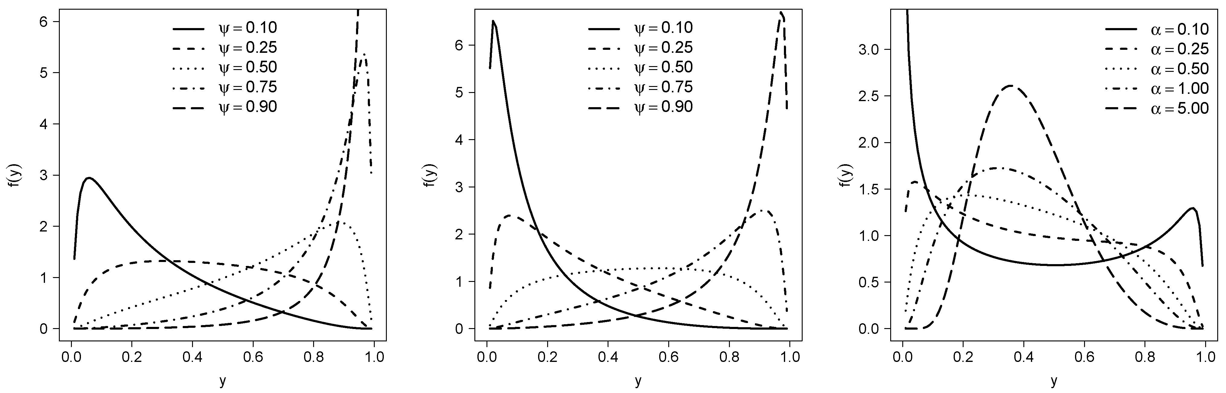
2. The Generalized Johnson Distribution
- We note that is the th quantile for the PGJSB model, where . Based on this idea, we also can reparametrize the model defining . The pdf for this reparametrization isIn this work, we will refer to this specific parametrization as RPGJSB1.
- Although is a parameter that needs to be estimated from the sample, we can consider , as fixed. With this definition, the cdf in (1) evaluated in is given by . Therefore, fixing , , we have that represents the th quantile of the distribution; further, as in the work of Lemonte and Bazán [9], also can be interpreted as a dispersion parameter. We will refer to this parametrization as RPGJSB2.
3. The Inference and Its Associated Diagnostic Analysis
3.1. Inference
3.2. Residuals
3.3. Local Influence
3.3.1. Perturbation of the Case Weights
3.3.2. Perturbation of the Response
3.3.3. Perturbation of the Predictor
4. Simulation Study
5. Data Analysis
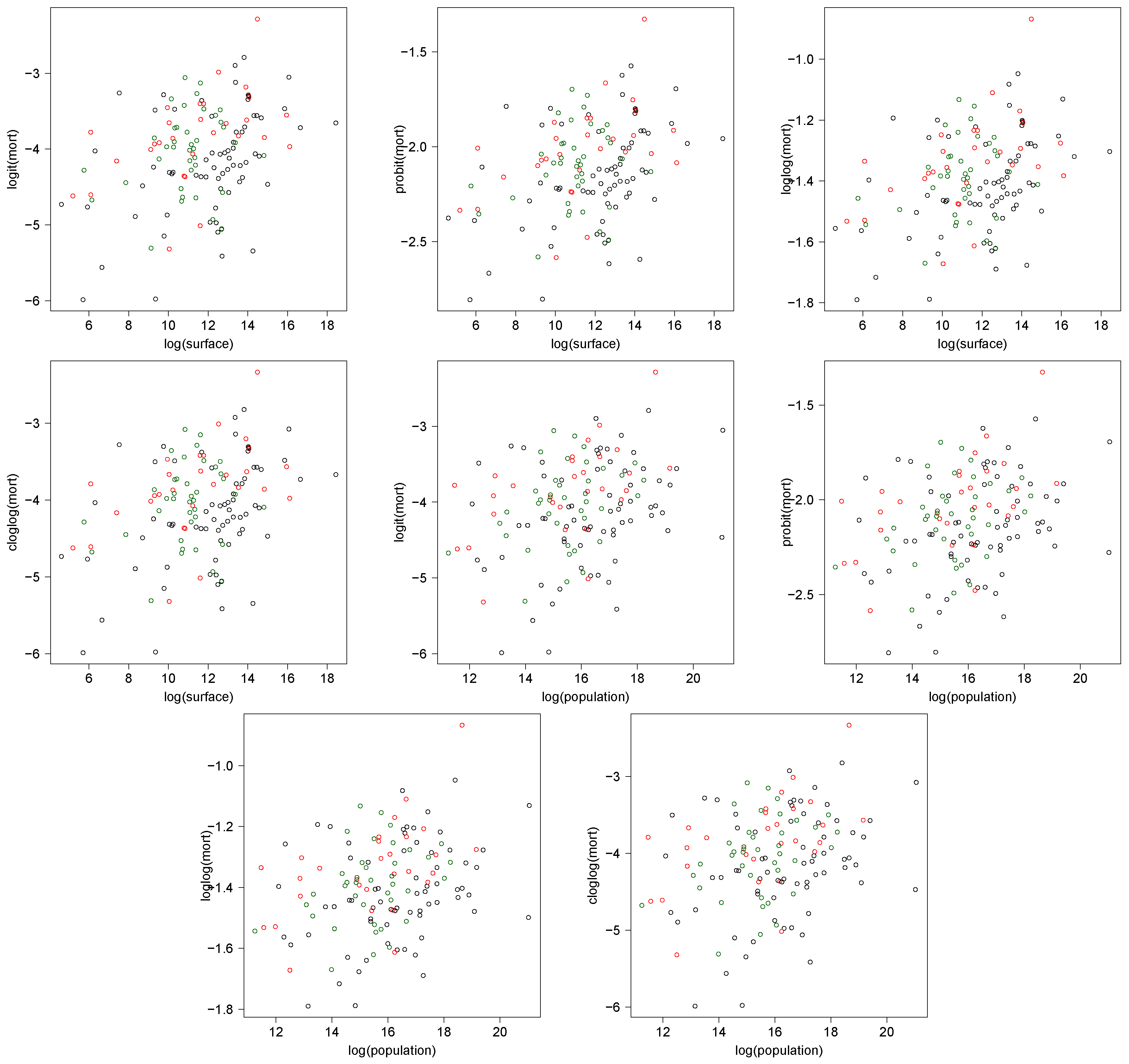
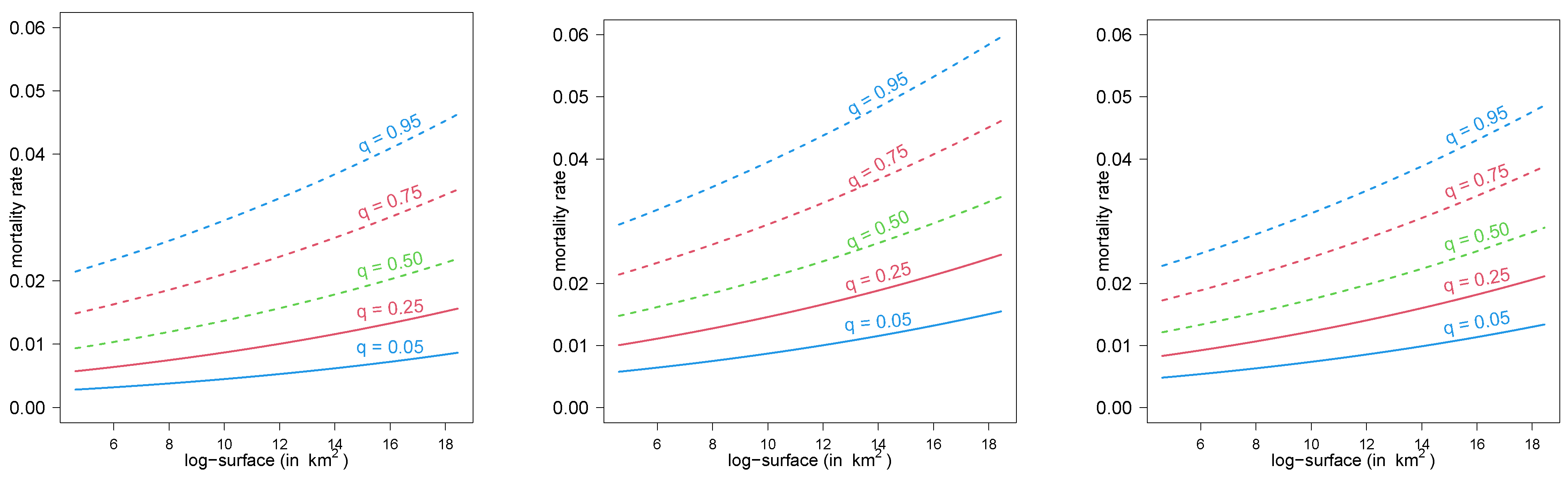
5.1. COVID-19 Data Set
- mort: mortality rate (reported deaths/reported cases since the pandemic started). Mean = 0.020, Median = 0.018, standard deviation = 0.013, minimum = 0.003, and maximum = 0.092.
- surface: area of the country (in km).
- population: official estimated population of the country.
- cont: continent to which the country belongs (categorized as 1: Africa, Asia, or Oceania; 2: the Americas; 3: Europe; with 69, 29, and 39 countries, respectively. This categorization was based on our previous analysis).
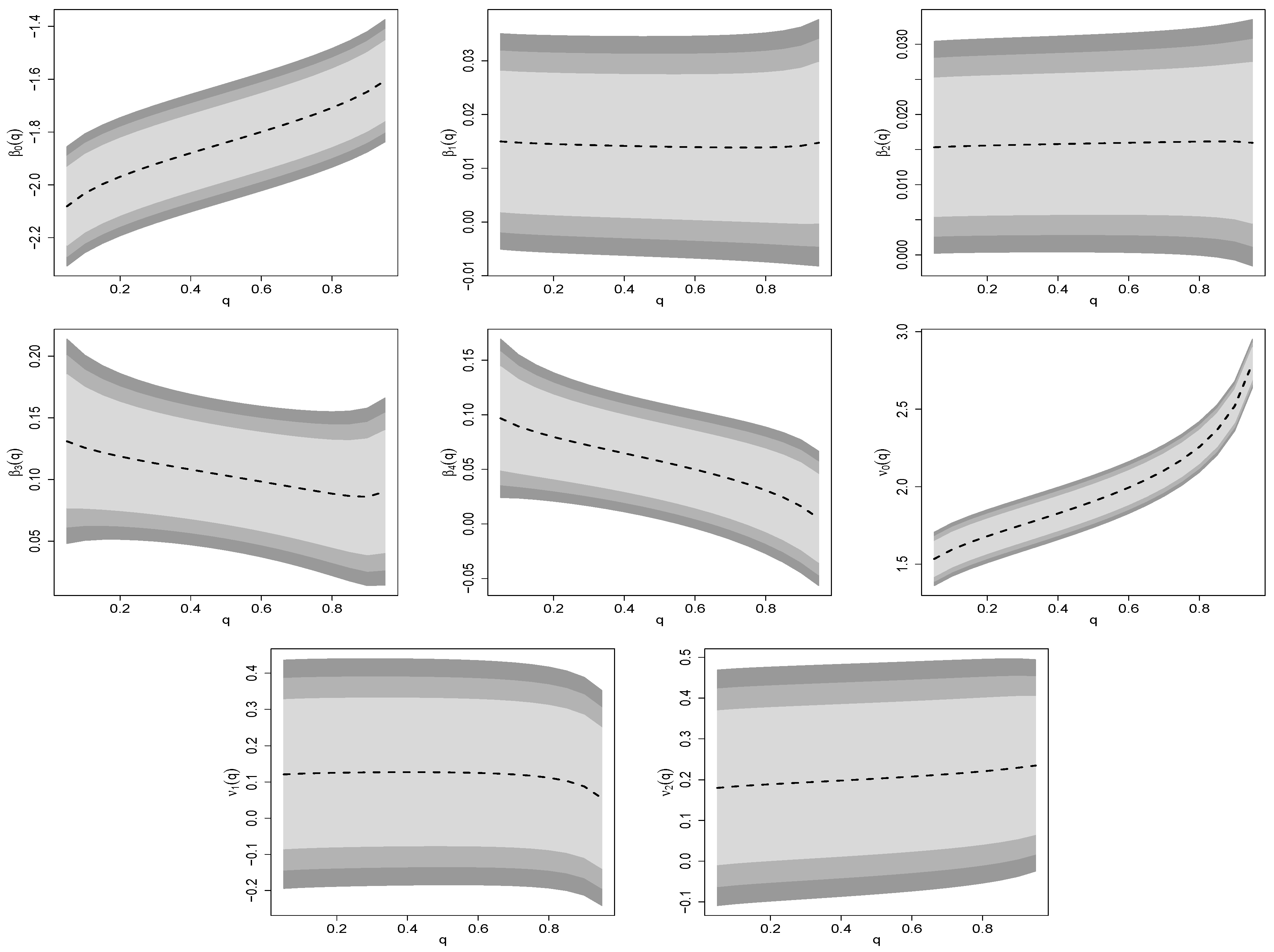
5.1.1. Estimation
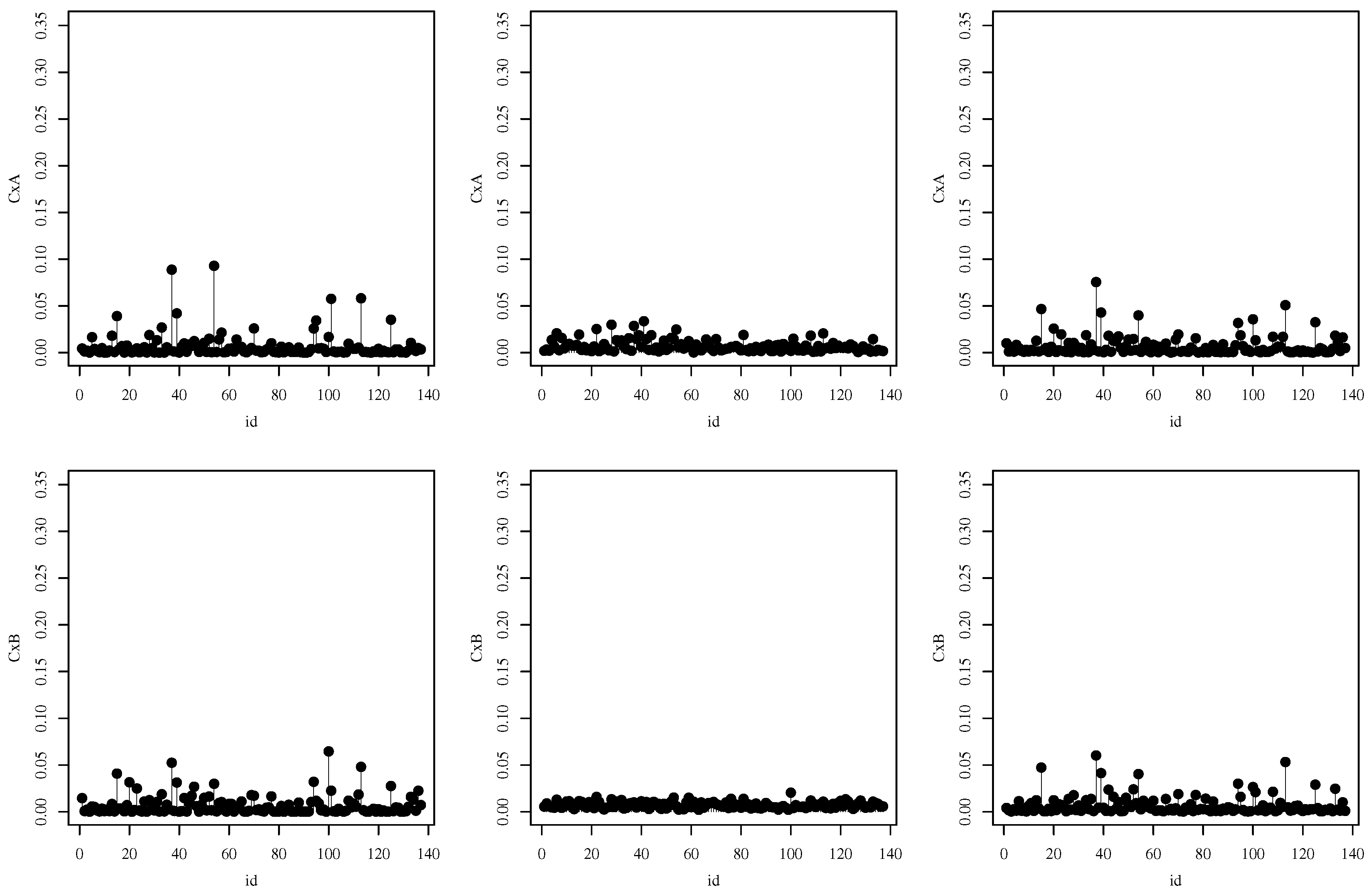
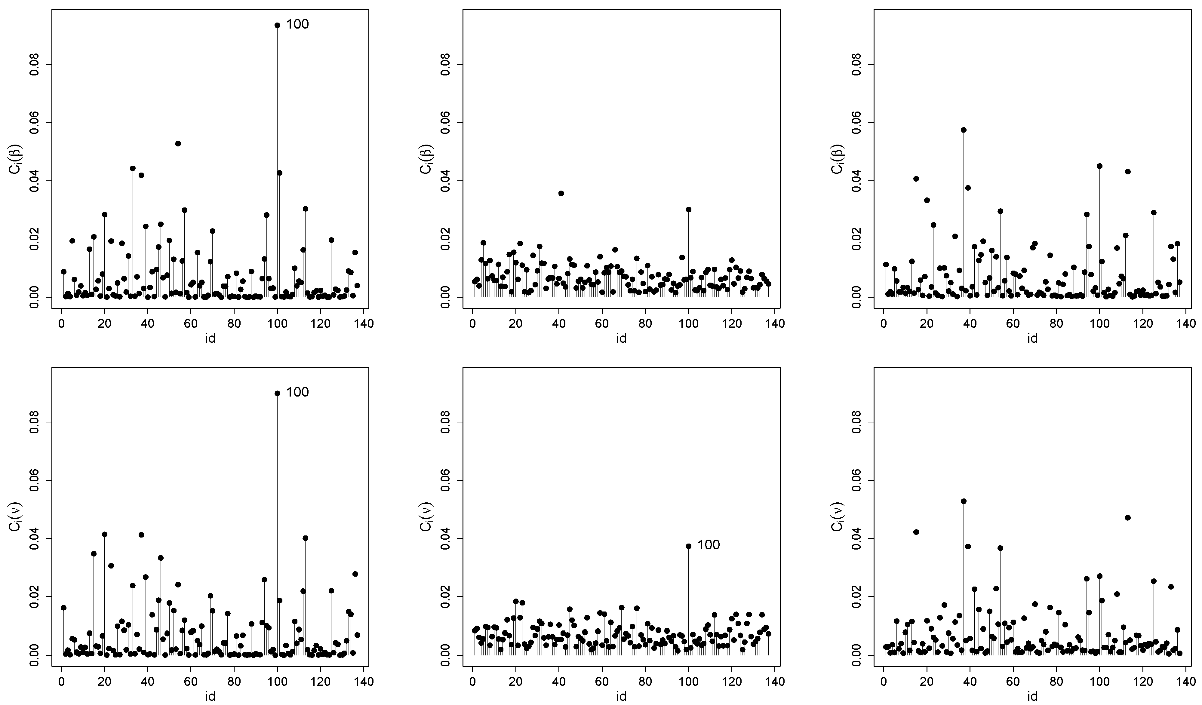
5.1.2. Local Influence Analysis
6. Conclusions
Author Contributions
Funding
Institutional Review Board Statement
Informed Consent Statement
Data Availability Statement
Conflicts of Interest
Abbreviations
| AD | Anderson–Darling (test) |
| AIC | Akaike information criterion |
| BIC | Bayesian information criterion |
| cdf | cumulative distribution function |
| CP | coverage probabilities |
| CVM | Cramér–Von-Mises (test) |
| GJS | generalized Johnson distribution |
| KS | Kolmogorov–Smirnov (test) |
| LD | likelihood displacement |
| ML | maximum likelihood |
| probability distribution function | |
| PJSB | power Johnson distribution |
| PGJSB | power generalized Johnson distribution |
| PGJSB1 | model 1 with reparametrization power generalized Johnson distribution |
| PGJSB2 | model 2 with reparametrization power generalized Johnson distribution |
| RQRs | randomized quantile residuals |
| SW | Shapiro–Wilks (test) |
Appendix A. Details of Local Influence
Appendix A.1. Perturbation of the Response
Appendix A.2. Perturbation of the Predictor
Appendix B. COVID-19 Data Set
Appendix B.1. AIC and BIC Criteria

| Normal | Logistic | Cauchy | |||||||||||
|---|---|---|---|---|---|---|---|---|---|---|---|---|---|
| Criteria | Logit | Probit | Loglog | Cloglog | Logit | Probit | Loglog | Cloglog | Logit | Probit | Loglog | Cloglog | |
| 0.05 | −871.9 | −871.7 | −871.5 | −871.9 | −871.4 | −871.3 | −871.3 | −871.3 | −840.3 | −841.5 | −842.4 | −840.1 | |
| 0.10 | −871.8 | −871.6 | −871.5 | −871.8 | −871.2 | −871.2 | −871.2 | −871.2 | −839.9 | −841.0 | −842.0 | −839.7 | |
| 0.15 | −871.7 | −871.6 | −871.5 | −871.8 | −871.2 | −871.2 | −871.1 | −871.2 | −839.7 | −840.8 | −841.8 | −839.5 | |
| 0.20 | −871.7 | −871.6 | −871.4 | −871.7 | −871.1 | −871.1 | −871.1 | −871.1 | −839.6 | −840.7 | −841.6 | −839.4 | |
| 0.25 | −871.6 | −871.5 | −871.4 | −871.7 | −871.1 | −871.1 | −871.1 | −871.1 | −839.5 | −840.6 | −841.6 | −839.3 | |
| 0.30 | −871.6 | −871.5 | −871.4 | −871.6 | −871.1 | −871.1 | −871.1 | −871.0 | −839.4 | −840.6 | −841.5 | −839.2 | |
| 0.35 | −871.5 | −871.5 | −871.4 | −871.6 | −871.0 | −871.0 | −871.0 | −871.0 | −839.4 | −840.5 | −841.5 | −839.2 | |
| 0.40 | −871.5 | −871.5 | −871.4 | −871.6 | −871.0 | −871.0 | −871.0 | −871.0 | −839.4 | −840.5 | −841.4 | −839.1 | |
| 0.45 | −871.5 | −871.4 | −871.3 | −871.5 | −871.0 | −871.0 | −871.0 | −870.9 | −839.3 | −840.5 | −841.4 | −839.1 | |
| AIC | 0.50 | −871.5 | −871.4 | −871.3 | −871.5 | −870.9 | −871.0 | −871.0 | −870.9 | −839.3 | −840.4 | −841.4 | −839.1 |
| 0.55 | −871.4 | −871.4 | −871.3 | −871.5 | −870.9 | −870.9 | −870.9 | −870.9 | −839.3 | −840.4 | −841.4 | −839.1 | |
| 0.60 | −871.4 | −871.4 | −871.3 | −871.5 | −870.9 | −870.9 | −870.9 | −870.9 | −839.3 | −840.4 | −841.3 | −839.0 | |
| 0.65 | −871.4 | −871.4 | −871.3 | −871.4 | −870.9 | −870.9 | −870.9 | −870.8 | −839.2 | −840.4 | −841.3 | −839.0 | |
| 0.70 | −871.3 | −871.3 | −871.3 | −871.4 | −870.8 | −870.9 | −870.9 | −870.8 | −839.2 | −840.3 | −841.3 | −839.0 | |
| 0.75 | −871.3 | −871.3 | −871.2 | −871.4 | −870.8 | −870.8 | −870.9 | −870.8 | −839.2 | −840.3 | −841.2 | −838.9 | |
| 0.80 | −871.3 | −871.3 | −871.2 | −871.3 | −870.8 | −870.8 | −870.8 | −870.8 | −839.1 | −840.2 | −841.2 | −838.9 | |
| 0.85 | −871.2 | −871.3 | −871.2 | −871.3 | −870.7 | −870.8 | −870.8 | −870.7 | −839.1 | −840.2 | −841.1 | −838.8 | |
| 0.90 | −871.2 | −871.2 | −871.2 | −871.3 | −870.7 | −870.7 | −870.7 | −870.7 | −839.0 | −840.1 | −841.1 | −838.8 | |
| 0.95 | −871.2 | −871.2 | −871.1 | −871.2 | −870.6 | −870.7 | −870.7 | −870.6 | −839.9 | −840.6 | −840.9 | −839.7 | |
| 0.05 | −839.7 | −839.6 | −839.4 | −839.8 | −839.2 | −839.2 | −839.1 | −839.2 | −808.2 | −809.4 | −810.3 | −808.0 | |
| 0.10 | −839.7 | −839.5 | −839.4 | −839.7 | −839.1 | −839.1 | −839.1 | −839.1 | −807.8 | −808.9 | −809.8 | −807.6 | |
| 0.15 | −839.6 | −839.5 | −839.3 | −839.7 | −839.1 | −839.0 | −839.0 | −839.0 | −807.6 | −808.7 | −809.6 | −807.4 | |
| 0.20 | −839.5 | −839.4 | −839.3 | −839.6 | −839.0 | −839.0 | −839.0 | −839.0 | −807.5 | −808.6 | −809.5 | −807.2 | |
| 0.25 | −839.5 | −839.4 | −839.3 | −839.6 | −839.0 | −839.0 | −839.0 | −838.9 | −807.4 | −808.5 | −809.5 | −807.2 | |
| 0.30 | −839.5 | −839.4 | −839.3 | −839.5 | −838.9 | −838.9 | −838.9 | −838.9 | −807.3 | −808.5 | −809.4 | −807.1 | |
| 0.35 | −839.4 | −839.4 | −839.3 | −839.5 | −838.9 | −838.9 | −838.9 | −838.9 | −807.3 | −808.4 | −809.4 | −807.1 | |
| 0.40 | −839.4 | −839.3 | −839.2 | −839.5 | −838.9 | −838.9 | −838.9 | −838.9 | −807.2 | −808.4 | −809.3 | −807.0 | |
| 0.45 | −839.4 | −839.3 | −839.2 | −839.4 | −838.8 | −838.9 | −838.9 | −838.8 | −807.2 | −808.4 | −809.3 | −807.0 | |
| BIC | 0.50 | −839.3 | −839.3 | −839.2 | −839.4 | −838.8 | −838.8 | −838.8 | −838.8 | −807.2 | −808.3 | −809.3 | −807.0 |
| 0.55 | −839.3 | −839.3 | −839.2 | −839.4 | −838.8 | −838.8 | −838.8 | −838.8 | −807.2 | −808.3 | −809.2 | −806.9 | |
| 0.60 | −839.3 | −839.3 | −839.2 | −839.3 | −838.8 | −838.8 | −838.8 | −838.7 | −807.1 | −808.3 | −809.2 | −806.9 | |
| 0.65 | −839.3 | −839.2 | −839.2 | −839.3 | −838.7 | −838.8 | −838.8 | −838.7 | −807.1 | −808.2 | −809.2 | −806.9 | |
| 0.70 | −839.2 | −839.2 | −839.1 | −839.3 | −838.7 | −838.7 | −838.8 | −838.7 | −807.1 | −808.2 | −809.2 | −806.8 | |
| 0.75 | −839.2 | −839.2 | −839.1 | −839.2 | −838.7 | −838.7 | −838.7 | −838.7 | −807.0 | −808.2 | −809.1 | −806.8 | |
| 0.80 | −839.2 | −839.2 | −839.1 | −839.2 | −838.7 | −838.7 | −838.7 | −838.6 | −807.0 | −808.1 | −809.1 | −806.8 | |
| 0.85 | −839.1 | −839.1 | −839.1 | −839.2 | −838.6 | −838.6 | −838.7 | −838.6 | −806.9 | −808.1 | −809.0 | −806.7 | |
| 0.90 | −839.1 | −839.1 | −839.0 | −839.1 | −838.6 | −838.6 | −838.6 | −838.6 | −806.9 | −808.0 | −808.9 | −806.7 | |
| 0.95 | −839.0 | −839.1 | −839.0 | −839.1 | −838.5 | −838.5 | −838.6 | −838.5 | −807.7 | −808.5 | −808.8 | −807.5 | |
| Normal | Logistic | Cauchy | |||||||||||
|---|---|---|---|---|---|---|---|---|---|---|---|---|---|
| Criteria | Logit | Probit | Loglog | Cloglog | Logit | Probit | Loglog | Cloglog | Logit | Probit | Loglog | Cloglog | |
| 0.05 | −869.0 | −872.3 | −873.4 | −868.7 | −857.4 | −863.8 | −867.6 | −856.9 | −758.5 | −770.5 | −779.3 | −757.6 | |
| 0.10 | −869.8 | −872.7 | −873.5 | −869.6 | −860.0 | −865.7 | −869.1 | −859.6 | −779.2 | −789.0 | −796.4 | −778.4 | |
| 0.15 | −870.4 | −872.9 | −873.5 | −870.1 | −862.1 | −867.2 | −870.1 | −861.7 | −795.1 | −803.3 | −809.4 | −794.5 | |
| 0.20 | −870.8 | −873.1 | −873.4 | −870.6 | −864.0 | −868.5 | −871.0 | −863.6 | −808.5 | −815.2 | −820.1 | −808.0 | |
| 0.25 | −871.2 | −873.2 | −873.4 | −871.0 | −865.7 | −869.7 | −871.8 | −865.3 | −819.6 | −825.0 | −828.9 | −819.1 | |
| 0.30 | −871.6 | −873.3 | −873.3 | −871.4 | −867.2 | −870.7 | −872.3 | −866.9 | −828.4 | −832.6 | −835.7 | −828.0 | |
| 0.35 | −871.9 | −873.4 | −873.1 | −871.7 | −868.7 | −871.6 | −872.8 | −868.4 | −835.0 | −838.1 | −840.4 | −834.6 | |
| 0.40 | −872.2 | −873.4 | −873.0 | −872.0 | −870.0 | −872.3 | −873.0 | −869.8 | −839.3 | −841.4 | −843.0 | −839.0 | |
| 0.45 | −872.4 | −873.4 | −872.8 | −872.3 | −871.2 | −872.7 | −872.9 | −871.0 | −841.2 | −842.5 | −843.3 | −841.0 | |
| AIC | 0.50 | −872.6 | −873.4 | −872.5 | −872.5 | −872.1 | −872.9 | −872.6 | −872.0 | −840.6 | −841.0 | −841.1 | −840.4 |
| 0.55 | −872.9 | −873.3 | −872.2 | −872.8 | −872.7 | −872.8 | −871.8 | −872.7 | −837.1 | −836.6 | −836.0 | −837.0 | |
| 0.60 | −873.0 | −873.2 | −871.8 | −873.0 | −872.9 | −872.0 | −870.4 | −872.9 | −830.1 | −828.7 | −827.5 | −830.1 | |
| 0.65 | −873.2 | −873.0 | −871.3 | −873.2 | −872.4 | −870.5 | −868.1 | −872.4 | −818.9 | −816.7 | −814.8 | −818.9 | |
| 0.70 | −873.3 | −872.7 | −870.8 | −873.3 | −870.8 | −867.9 | −864.6 | −871.0 | −802.3 | −799.2 | −796.6 | −802.4 | |
| 0.75 | −873.3 | −872.3 | −870.0 | −873.4 | −867.7 | −863.5 | −859.3 | −868.0 | −778.5 | −774.5 | −771.2 | −778.6 | |
| 0.80 | −873.2 | −871.7 | −868.9 | −873.3 | −862.2 | −856.5 | −851.1 | −862.6 | −744.2 | −739.3 | −735.4 | −744.3 | |
| 0.85 | −873.0 | −870.8 | −867.5 | −873.1 | −852.8 | −845.3 | −838.5 | −853.3 | −693.1 | −687.5 | −682.9 | −693.4 | |
| 0.90 | −872.3 | −869.3 | −865.2 | −872.5 | −836.9 | −827.1 | −818.5 | −837.6 | −611.5 | −605.2 | −600.1 | −611.8 | |
| 0.95 | −870.7 | −866.3 | −861.1 | −871.1 | −810.5 | −797.4 | −786.0 | −811.6 | −453.7 | −446.8 | −431.4 | −454.1 | |
| 0.05 | −839.8 | −843.1 | −844.2 | −839.5 | −828.2 | −834.6 | −838.4 | −827.7 | −729.3 | −741.3 | −750.1 | −728.4 | |
| 0.10 | −840.6 | −843.5 | −844.3 | −840.4 | −830.8 | −836.5 | −839.9 | −830.4 | −750.0 | −759.8 | −767.2 | −749.2 | |
| 0.15 | −841.2 | −843.7 | −844.3 | −840.9 | −832.9 | −838.0 | −840.9 | −832.5 | −765.9 | −774.1 | −780.2 | −765.3 | |
| 0.20 | −841.6 | −843.9 | −844.2 | −841.4 | −834.8 | −839.3 | −841.8 | −834.4 | −779.3 | −786.0 | −790.9 | −778.8 | |
| 0.25 | −842.0 | −844.0 | −844.2 | −841.8 | −836.5 | −840.5 | −842.6 | −836.1 | −790.4 | −795.8 | −799.7 | −789.9 | |
| 0.30 | −842.4 | −844.1 | −844.1 | −842.2 | −838.0 | −841.5 | −843.1 | −837.7 | −799.2 | −803.4 | −806.5 | −798.8 | |
| 0.35 | −842.7 | −844.2 | −843.9 | −842.5 | −839.5 | −842.4 | −843.6 | −839.2 | −805.8 | −808.9 | −811.2 | −805.4 | |
| 0.40 | −843.0 | −844.2 | −843.8 | −842.8 | −840.8 | −843.1 | −843.8 | −840.6 | −810.1 | −812.2 | −813.8 | −809.8 | |
| 0.45 | −843.2 | −844.2 | −843.6 | −843.1 | −842.0 | −843.5 | −843.7 | −841.8 | −812.0 | −813.3 | −814.1 | −811.8 | |
| BIC | 0.50 | −843.4 | −844.2 | −843.3 | −843.3 | −842.9 | −843.7 | −843.4 | −842.8 | −811.4 | −811.8 | −811.9 | −811.2 |
| 0.55 | −843.7 | −844.1 | −843.0 | −843.6 | −843.5 | −843.6 | −842.6 | −843.5 | −807.9 | −807.4 | −806.8 | −807.8 | |
| 0.60 | −843.8 | −844.0 | −842.6 | −843.8 | −843.7 | −842.8 | −841.2 | −843.7 | −800.9 | −799.5 | −798.3 | −800.9 | |
| 0.65 | −844.0 | −843.8 | −842.1 | −844.0 | −843.2 | −841.3 | −838.9 | −843.2 | −789.7 | −787.5 | −785.6 | −789.7 | |
| 0.70 | −844.1 | −843.5 | −841.6 | −844.1 | −841.6 | −838.7 | −835.4 | −841.8 | −773.1 | −770.0 | −767.4 | −773.2 | |
| 0.75 | −844.1 | −843.1 | −840.8 | −844.2 | −838.5 | −834.3 | −830.1 | −838.8 | −749.3 | −745.3 | −742.0 | −749.4 | |
| 0.80 | −844.0 | −842.5 | −839.7 | −844.1 | −833.0 | −827.3 | −821.9 | −833.4 | −715.0 | −710.1 | −706.2 | −715.1 | |
| 0.85 | −843.8 | −841.6 | −838.3 | −843.9 | −823.6 | −816.1 | −809.3 | −824.1 | −663.9 | −658.3 | −653.7 | −664.2 | |
| 0.90 | −843.1 | −840.1 | −836.0 | −843.3 | −807.7 | −797.9 | −789.3 | −808.4 | −582.3 | −576.0 | −570.9 | −582.6 | |
| 0.95 | −841.5 | −837.1 | −831.9 | −841.9 | −781.3 | −768.2 | −756.8 | −782.4 | −424.5 | −417.6 | −402.2 | −424.9 | |
Appendix B.2. Estimated Parameters
| p-Values for Quantile Residuals | |||||||||
|---|---|---|---|---|---|---|---|---|---|
| Parameter | Estimated | s.e. | t-Value | p-Value | KS | SW | AD | CVM | |
| 0.1 | −2.0810 | 0.1154 | −18.03 | <0.0001 | 0.441 | 0.260 | 0.128 | 0.099 | |
| 0.0150 | 0.0102 | 1.46 | 0.0716 | ||||||
| 0.0153 | 0.0077 | 1.99 | 0.0234 | ||||||
| 0.1310 | 0.0423 | 3.10 | 0.0010 | ||||||
| 0.0967 | 0.0371 | 2.61 | 0.0045 | ||||||
| 1.5341 | 0.0881 | 17.41 | <0.0001 | ||||||
| 0.1210 | 0.1608 | 0.75 | 0.2259 | ||||||
| 0.1801 | 0.1474 | 1.22 | 0.1110 | ||||||
| 0.25 | −1.9443 | 0.1140 | −17.06 | <0.0001 | 0.573 | 0.324 | 0.164 | 0.119 | |
| 0.0144 | 0.0103 | 1.40 | 0.0814 | ||||||
| 0.0156 | 0.0078 | 2.01 | 0.0223 | ||||||
| 0.1158 | 0.0331 | 3.50 | 0.0002 | ||||||
| 0.0756 | 0.0290 | 2.61 | 0.0046 | ||||||
| 1.7178 | 0.0873 | 19.69 | <0.0001 | ||||||
| 0.1263 | 0.1600 | 0.79 | 0.2149 | ||||||
| 0.1914 | 0.1462 | 1.31 | 0.0953 | ||||||
| 0.75 | −1.7334 | 0.1144 | −15.16 | <0.0001 | 0.396 | 0.070 | 0.048 | 0.035 | |
| 0.0139 | 0.0108 | 1.29 | 0.0989 | ||||||
| 0.0161 | 0.0082 | 1.97 | 0.0244 | ||||||
| 0.0909 | 0.0330 | 2.76 | 0.0029 | ||||||
| 0.0364 | 0.0289 | 1.26 | 0.1041 | ||||||
| 2.1731 | 0.0843 | 25.78 | <0.0001 | ||||||
| 0.1174 | 0.1564 | 0.75 | 0.2264 | ||||||
| 0.2170 | 0.1412 | 1.54 | 0.0622 | ||||||
| 0.9 | -1.6473 | 0.1163 | −14.16 | <0.0001 | 0.169 | 0.005 | 0.006 | 0.005 | |
| 0.0142 | 0.0113 | 1.26 | 0.1044 | ||||||
| 0.0161 | 0.0086 | 1.87 | 0.0304 | ||||||
| 0.0860 | 0.0367 | 2.34 | 0.0096 | ||||||
| 0.0162 | 0.0311 | 0.52 | 0.3018 | ||||||
| 2.5206 | 0.0818 | 30.81 | <0.0001 | ||||||
| 0.0877 | 0.1534 | 0.57 | 0.2837 | ||||||
| 0.2296 | 0.1363 | 1.68 | 0.0460 | ||||||
Appendix B.3. Additional Information for Local Influence


References
- Ferrari, S.L.; Cribari-Neto, F. Beta regression for modelling rates and proportions. J. Appl. Stat. 2004, 31, 799–815. [Google Scholar] [CrossRef]
- Ospina, R.; Ferrari, S.L.P. Inflated beta distributions. Stat. Pap. 2008, 51, 111–126. [Google Scholar] [CrossRef] [Green Version]
- Bayes, C.L.; Bazán, J.L.; García, C. A new robust regression model for proportions. Bayesian Anal. 2012, 7, 841–866. [Google Scholar] [CrossRef]
- Migliorati, S.; Di Brisco, A.M.; Ongaro, A. A New Regression Model for Bounded Responses. Bayesian Anal. 2018, 13, 845–872. [Google Scholar] [CrossRef]
- Koenker, R.; Bassett, G. Regression quantiles. Econometrica 1978, 46, 33–50. [Google Scholar] [CrossRef]
- Lemonte, A.J.; Moreno-Arenas, G. On a heavy-tailed parametric quantile regression model for limited range response variables. Comput. Stat. 2020, 35, 379–398. [Google Scholar] [CrossRef]
- Su, S. Flexible parametric quantile regression model. Stat. Comput. 2015, 25, 635–650. [Google Scholar] [CrossRef]
- Mazucheli, J.; Menezes, A.F.B.; Fernandes, L.B.; Oliveira, R.P.; Ghitany, M.E. The unit-Weibull distribution as an alternative to the Kumaraswamy distribution for the modelling of quantiles conditional on covariates. J. Appl. Stat. 2020, 47, 954–974. [Google Scholar] [CrossRef]
- Lemonte, A.J.; Bazán, J.L. New class of Johnson SB distributions and its associated regression model for rates and proportions. Biom. J. 2016, 58, 727–746. [Google Scholar] [CrossRef] [PubMed]
- Johnson, N.L. Systems of frequency curves generated by the methods of translation. Biometrika 1949, 36, 149–176. [Google Scholar] [CrossRef]
- Cancho, V.G.; Bazán, J.L.; Dey, D.K. A new class of regression model for a bounded response with application in the study of the incidence rate of colorectal cancer. Stat. Methods Med. Res. 2020, 29, 2015–2033. [Google Scholar] [CrossRef] [PubMed]
- Bayes, C.L.; Bazán, J.L.; De Castro, M. A quantile parametric mixed regression model for bounded response variables. Stat. Interface 2017, 10, 483–493. [Google Scholar] [CrossRef]
- Durrans, S.R. Distributions of fractional order statistics in hydrology. Water Resour. Res. 1992, 28, 1649–1655. [Google Scholar] [CrossRef]
- Lehmann, E.L. The power of rank tests. Ann. Math. Stat. 1953, 24, 23–43. [Google Scholar] [CrossRef]
- Fletcher, R. Practical Methods of Optimization, 2nd ed.; John Wiley & Sons.: New York, NY, USA, 1987. [Google Scholar]
- Cox, D.; Hinkley, D. Theoretical Statistics; Chapman and Hall: London, UK, 1974. [Google Scholar]
- Dunn, P.K.; Smyth, G.K. Randomized quantile residuals. J. Comput. Graph. Stat. 1996, 5, 236–244. [Google Scholar]
- Yap, B.W.; Sim, C.H. Comparisons of various normality tests. J. Stat. Comput. Simul. 2011, 81, 2141–2155. [Google Scholar] [CrossRef]
- Cook, R.D. Assessment of Local Influence. J. R. Soc. B Stat. Methodol. 1986, 48, 133–155. [Google Scholar] [CrossRef]
- R Core Team. R: A Language and Environment for Statistical Computing; R Foundation for Statistical Computing: Vienna, Austria, 2021; Available online: https://www.R-project.org/ (accessed on 10 January 2022).
- Du, R.H.; Liang, L.R.; Yang, C.Q.; Wang, W.; Cao, T.Z.; Li, M.; Guo, G.Y.; Du, J.; Zheng, C.L.; Zhu, Q.; et al. Predictors of mortality for patients with COVID-19 pneumonia caused by SARS-CoV-2: A prospective cohort study. Eur. Respir. J. 2020, 55, 2000524. [Google Scholar] [CrossRef] [Green Version]
- Ji, J.S.; Liu, Y.; Liu, R.; Zha, Y.; Chang, X.; Zhang, L.; Zhang, Y.; Zeng, J.; Dong, T.; Xu, X.; et al. Survival analysis of hospital length of stay of novel coronavirus (COVID-19) pneumonia patients in Sichuan, China. medRxiv 2020. [Google Scholar] [CrossRef]
- Li, X.; Xu, S.; Yu, M.; Wang, K.; Tao, Y.; Zhou, Y.; Shi, J.; Zhou, M.; Wu, B.; Yang, Z. Risk factors for severity and mortality in adult COVID-19 inpatients in Wuhan. J. Allergy Clin. Immunol. 2020, 146, 110–118. [Google Scholar] [CrossRef]
- Livingston, E.; Bucher, K. Coronavirus disease 2019 (COVID-19) in Italy. J. Am. Med Assoc. 2020, 323, 1335. [Google Scholar] [CrossRef] [PubMed] [Green Version]
- WHO. Coronavirus Disease (COVID-19) Dashboard; World Health Organization: Geneva, Switzerland, 2021; Available online: https://covid19.who.int/ (accessed on 25 May 2021).


| Logistic | Normal | ||||||||||
|---|---|---|---|---|---|---|---|---|---|---|---|
| Link | |||||||||||
| logit | 0.1 | 4.9 | 2.6 | 2.2 | 0.4 | −0.7 | 4.4 | 2.4 | 1.5 | 0.3 | −1.4 |
| 0.5 | 4.8 | 2.1 | 2.2 | 0.4 | −0.7 | 4.6 | 2.1 | 1.5 | 0.3 | −1.4 | |
| 0.9 | 4.7 | 1.8 | 2.2 | 0.4 | −0.7 | 4.8 | 1.9 | 1.5 | 0.3 | −1.4 | |
| loglog | 0.1 | 1.3 | 0.8 | 0.8 | −0.3 | 0.1 | 1.2 | 0.7 | −0.1 | −0.3 | 1.1 |
| 0.5 | 2.1 | 0.9 | 1.0 | −0.2 | 0.1 | 2.0 | 0.9 | 0.0 | −0.3 | 1.0 | |
| 0.9 | 2.8 | 1.0 | 1.1 | −0.2 | 0.1 | 2.8 | 1.0 | 0.1 | −0.2 | 1.0 | |
| Link | Parameter | Bias | CP | Bias | CP | Bias | CP | ||||||||
| logistic | logit | 0.1 | −0.034 | 0.753 | 0.728 | 0.938 | −0.017 | 0.538 | 0.529 | 0.946 | −0.007 | 0.345 | 0.339 | 0.946 | |
| −0.015 | 0.238 | 0.229 | 0.934 | −0.007 | 0.166 | 0.163 | 0.942 | −0.003 | 0.104 | 0.102 | 0.947 | ||||
| 0.041 | 0.381 | 0.367 | 0.935 | 0.020 | 0.269 | 0.263 | 0.942 | 0.009 | 0.171 | 0.170 | 0.947 | ||||
| −0.001 | 0.088 | 0.085 | 0.939 | 0.000 | 0.061 | 0.060 | 0.946 | 0.000 | 0.039 | 0.038 | 0.946 | ||||
| −0.004 | 0.355 | 0.331 | 0.947 | −0.002 | 0.232 | 0.224 | 0.946 | −0.002 | 0.140 | 0.138 | 0.948 | ||||
| 0.5 | −0.017 | 0.485 | 0.472 | 0.941 | 0.001 | 0.322 | 0.319 | 0.946 | −0.003 | 0.204 | 0.205 | 0.950 | |||
| −0.005 | 0.146 | 0.142 | 0.939 | 0.000 | 0.096 | 0.095 | 0.946 | −0.001 | 0.061 | 0.061 | 0.949 | ||||
| 0.046 | 0.452 | 0.443 | 0.946 | 0.027 | 0.296 | 0.294 | 0.948 | 0.007 | 0.183 | 0.182 | 0.949 | ||||
| 0.002 | 0.107 | 0.106 | 0.946 | 0.002 | 0.068 | 0.068 | 0.949 | 0.000 | 0.042 | 0.042 | 0.951 | ||||
| 0.004 | 0.352 | 0.331 | 0.952 | −0.001 | 0.231 | 0.224 | 0.948 | 0.000 | 0.142 | 0.139 | 0.947 | ||||
| 0.9 | −0.001 | 0.620 | 0.591 | 0.930 | −0.002 | 0.369 | 0.363 | 0.942 | 0.002 | 0.237 | 0.236 | 0.950 | |||
| 0.004 | 0.177 | 0.169 | 0.932 | 0.002 | 0.112 | 0.111 | 0.943 | 0.001 | 0.072 | 0.072 | 0.948 | ||||
| 0.060 | 0.461 | 0.443 | 0.943 | 0.024 | 0.289 | 0.283 | 0.943 | 0.007 | 0.184 | 0.182 | 0.946 | ||||
| 0.006 | 0.103 | 0.100 | 0.938 | 0.002 | 0.066 | 0.065 | 0.946 | 0.000 | 0.043 | 0.043 | 0.945 | ||||
| 0.010 | 0.362 | 0.334 | 0.946 | 0.003 | 0.234 | 0.224 | 0.949 | 0.002 | 0.140 | 0.139 | 0.949 | ||||
| loglog | 0.1 | 0.008 | 0.175 | 0.168 | 0.931 | 0.002 | 0.116 | 0.113 | 0.938 | 0.000 | 0.071 | 0.071 | 0.949 | ||
| 0.001 | 0.039 | 0.037 | 0.935 | 0.000 | 0.026 | 0.025 | 0.937 | 0.000 | 0.016 | 0.016 | 0.948 | ||||
| 0.020 | 0.413 | 0.398 | 0.944 | 0.005 | 0.280 | 0.275 | 0.946 | −0.001 | 0.165 | 0.167 | 0.950 | ||||
| 0.000 | 0.096 | 0.092 | 0.939 | −0.002 | 0.067 | 0.065 | 0.942 | −0.001 | 0.039 | 0.039 | 0.949 | ||||
| 0.153 | 1.175 | 2.515 | 0.964 | 0.035 | 0.349 | 0.324 | 0.961 | 0.014 | 0.178 | 0.174 | 0.956 | ||||
| 0.5 | −0.002 | 0.130 | 0.128 | 0.944 | −0.003 | 0.090 | 0.090 | 0.951 | 0.001 | 0.061 | 0.061 | 0.946 | |||
| 0.000 | 0.031 | 0.030 | 0.945 | −0.001 | 0.021 | 0.021 | 0.949 | 0.000 | 0.014 | 0.014 | 0.947 | ||||
| 0.007 | 0.386 | 0.376 | 0.944 | 0.003 | 0.264 | 0.261 | 0.947 | 0.006 | 0.175 | 0.175 | 0.950 | ||||
| −0.003 | 0.093 | 0.091 | 0.945 | −0.002 | 0.063 | 0.062 | 0.949 | 0.000 | 0.041 | 0.041 | 0.950 | ||||
| 0.143 | 1.070 | 2.042 | 0.965 | 0.041 | 0.306 | 0.290 | 0.962 | 0.012 | 0.177 | 0.174 | 0.951 | ||||
| 0.9 | −0.005 | 0.178 | 0.175 | 0.939 | −0.004 | 0.141 | 0.139 | 0.942 | −0.002 | 0.082 | 0.082 | 0.947 | |||
| −0.001 | 0.042 | 0.041 | 0.940 | −0.001 | 0.033 | 0.032 | 0.943 | 0.000 | 0.019 | 0.019 | 0.947 | ||||
| 0.012 | 0.387 | 0.374 | 0.940 | 0.010 | 0.296 | 0.288 | 0.944 | 0.004 | 0.174 | 0.173 | 0.949 | ||||
| −0.002 | 0.094 | 0.091 | 0.940 | 0.000 | 0.071 | 0.069 | 0.944 | 0.000 | 0.041 | 0.041 | 0.949 | ||||
| 0.133 | 0.968 | 1.596 | 0.965 | 0.042 | 0.311 | 0.290 | 0.961 | 0.014 | 0.177 | 0.174 | 0.952 | ||||
| Link | Parameter | Bias | CP | Bias | CP | Bias | CP | ||||||||
| normal | logit | 0.1 | −0.004 | 0.725 | 0.711 | 0.939 | 0.000 | 0.470 | 0.473 | 0.952 | −0.002 | 0.289 | 0.291 | 0.951 | |
| −0.005 | 0.202 | 0.198 | 0.939 | −0.002 | 0.133 | 0.134 | 0.951 | −0.002 | 0.081 | 0.082 | 0.949 | ||||
| 0.912 | 2.171 | 0.730 | 0.847 | 0.243 | 1.024 | 0.450 | 0.946 | 0.045 | 0.270 | 0.248 | 0.954 | ||||
| 0.000 | 0.083 | 0.079 | 0.932 | 0.001 | 0.055 | 0.054 | 0.945 | 0.000 | 0.032 | 0.032 | 0.951 | ||||
| −1.763 | 4.569 | 1.650 | 0.867 | −0.462 | 2.167 | 1.019 | 0.960 | −0.082 | 0.612 | 0.565 | 0.956 | ||||
| 0.5 | −0.006 | 0.464 | 0.452 | 0.942 | −0.005 | 0.330 | 0.324 | 0.945 | 0.002 | 0.196 | 0.194 | 0.946 | |||
| −0.004 | 0.135 | 0.131 | 0.940 | −0.002 | 0.094 | 0.092 | 0.941 | 0.000 | 0.056 | 0.056 | 0.946 | ||||
| 0.944 | 2.251 | 0.703 | 0.841 | 0.215 | 0.966 | 0.450 | 0.949 | 0.040 | 0.281 | 0.250 | 0.952 | ||||
| 0.002 | 0.082 | 0.079 | 0.939 | 0.001 | 0.056 | 0.055 | 0.947 | 0.000 | 0.034 | 0.033 | 0.950 | ||||
| −1.806 | 4.729 | 1.597 | 0.862 | −0.398 | 2.046 | 1.012 | 0.961 | −0.071 | 0.625 | 0.564 | 0.954 | ||||
| 0.9 | −0.028 | 0.595 | 0.550 | 0.910 | −0.001 | 0.393 | 0.375 | 0.934 | −0.004 | 0.244 | 0.242 | 0.947 | |||
| −0.002 | 0.165 | 0.153 | 0.912 | 0.003 | 0.111 | 0.106 | 0.933 | 0.000 | 0.069 | 0.069 | 0.949 | ||||
| 0.923 | 2.248 | 0.712 | 0.852 | 0.235 | 1.009 | 0.450 | 0.947 | 0.047 | 0.279 | 0.253 | 0.949 | ||||
| 0.006 | 0.088 | 0.084 | 0.937 | 0.001 | 0.057 | 0.055 | 0.941 | 0.001 | 0.035 | 0.035 | 0.949 | ||||
| −1.733 | 4.706 | 1.576 | 0.871 | −0.434 | 2.133 | 1.008 | 0.961 | −0.083 | 0.614 | 0.563 | 0.956 | ||||
| loglog | 0.1 | 0.005 | 0.156 | 0.152 | 0.935 | 0.005 | 0.115 | 0.114 | 0.942 | 0.001 | 0.070 | 0.069 | 0.946 | ||
| 0.000 | 0.035 | 0.034 | 0.936 | 0.001 | 0.026 | 0.026 | 0.945 | 0.000 | 0.016 | 0.015 | 0.946 | ||||
| 0.085 | 0.834 | 0.530 | 0.963 | 0.024 | 0.371 | 0.351 | 0.951 | 0.006 | 0.209 | 0.209 | 0.952 | ||||
| −0.004 | 0.077 | 0.076 | 0.942 | −0.001 | 0.059 | 0.058 | 0.946 | −0.001 | 0.035 | 0.035 | 0.951 | ||||
| 1.090 | 23.978 | 3.284 | 0.965 | 0.103 | 1.677 | 1.200 | 0.958 | 0.027 | 0.661 | 0.658 | 0.961 | ||||
| 0.5 | 0.002 | 0.116 | 0.114 | 0.942 | 0.000 | 0.084 | 0.083 | 0.946 | 0.000 | 0.054 | 0.053 | 0.948 | |||
| 0.000 | 0.026 | 0.025 | 0.942 | 0.000 | 0.019 | 0.019 | 0.947 | 0.000 | 0.012 | 0.012 | 0.947 | ||||
| 0.123 | 0.990 | 0.539 | 0.954 | 0.017 | 0.379 | 0.348 | 0.955 | 0.009 | 0.212 | 0.212 | 0.952 | ||||
| −0.004 | 0.082 | 0.079 | 0.939 | −0.002 | 0.059 | 0.059 | 0.946 | −0.001 | 0.036 | 0.036 | 0.950 | ||||
| 0.612 | 16.917 | 3.114 | 0.964 | 0.091 | 1.453 | 1.150 | 0.963 | 0.017 | 0.654 | 0.645 | 0.957 | ||||
| 0.9 | −0.016 | 0.224 | 0.219 | 0.935 | −0.007 | 0.169 | 0.167 | 0.939 | −0.004 | 0.095 | 0.095 | 0.943 | |||
| −0.002 | 0.051 | 0.050 | 0.937 | −0.001 | 0.040 | 0.039 | 0.940 | −0.001 | 0.022 | 0.022 | 0.946 | ||||
| 0.125 | 0.934 | 0.538 | 0.958 | 0.029 | 0.386 | 0.357 | 0.951 | 0.008 | 0.208 | 0.207 | 0.951 | ||||
| 0.000 | 0.083 | 0.080 | 0.940 | 0.000 | 0.061 | 0.060 | 0.948 | 0.000 | 0.035 | 0.034 | 0.952 | ||||
| 0.428 | 12.877 | 2.696 | 0.964 | 0.088 | 1.443 | 1.192 | 0.957 | 0.034 | 0.657 | 0.647 | 0.961 | ||||
| Link | 100 | 200 | 500 | 100 | 200 | 500 | 100 | 200 | 500 | |
| logistic | logit | 100.00 | 100.00 | 100.00 | 100.00 | 100.00 | 100.00 | 100.00 | 100.00 | 100.00 |
| loglog | 99.71 | 100.00 | 100.00 | 99.83 | 100.00 | 100.00 | 99.85 | 100.00 | 100.00 | |
| normal | logit | 90.77 | 98.40 | 100.00 | 89.43 | 98.65 | 99.99 | 90.38 | 98.59 | 99.99 |
| loglog | 99.43 | 99.99 | 100.00 | 99.01 | 99.98 | 100.00 | 99.05 | 99.98 | 100.00 | |
| p-Values for Quantile Residuals | |||||||||
|---|---|---|---|---|---|---|---|---|---|
| Parameter | Estimated | s.e. | -Value | -Value | KS | SW | AD | CVM | |
| 0.5 | −1.8396 | 0.1136 | −16.19 | <0.0001 | 0.626 | 0.249 | 0.133 | 0.094 | |
| 0.0140 | 0.0105 | 1.34 | 0.0899 | ||||||
| 0.0159 | 0.0079 | 2.01 | 0.0223 | ||||||
| 0.1032 | 0.0308 | 3.35 | 0.0004 | ||||||
| 0.0575 | 0.0272 | 2.12 | 0.0171 | ||||||
| 1.9051 | 0.0862 | 22.11 | <0.0001 | ||||||
| 0.1268 | 0.1587 | 0.80 | 0.2121 | ||||||
| 0.2028 | 0.1445 | 1.40 | 0.0802 | ||||||
| q | ||||||
|---|---|---|---|---|---|---|
| Parameter | 0.10 | 0.25 | 0.50 | 0.75 | 0.90 | |
| RC | 239.95 | 243.30 | 253.85 | 267.69 | 279.66 | |
| RCSE | 18.10 | 18.71 | 19.62 | 20.63 | 21.45 | |
| p-value | <0.0001 | <0.0001 | <0.0001 | <0.0001 | <0.0001 | |
| RC | 298.10 | 295.33 | 296.05 | 292.45 | 276.05 | |
| RCSE | 224.15 | 228.55 | 233.01 | 233.17 | 223.76 | |
| p-value | 0.1751 | 0.1879 | 0.1979 | 0.2067 | 0.2151 | |
| RC | 313.98 | 310.46 | 305.38 | 300.83 | 300.56 | |
| RCSE | 161.89 | 158.80 | 155.11 | 150.94 | 147.41 | |
| p-value | 0.0508 | 0.0491 | 0.0479 | 0.0469 | 0.046 | |
| RC | 398.39 | 402.09 | 431.38 | 472.57 | 475.72 | |
| RCSE | 104.18 | 103.37 | 108.53 | 113.21 | 109.20 | |
| p-value | 0.0002 | 0.0001 | 0.0001 | 0.0001 | 0.0002 | |
| RC | 406.56 | 446.90 | 569.98 | 895.37 | 2014.00 | |
| RCSE | 139.08 | 150.33 | 184.91 | 270.23 | 566.60 | |
| p-value | 0.0041 | 0.0037 | 0.0039 | 0.0044 | 0.0054 | |
| RC | 96.05 | 92.62 | 90.77 | 89.93 | 89.73 | |
| RCSE | 0.02 | 0.01 | 0.06 | 0.13 | 0.21 | |
| p-value | 0.4717 | 0.1467 | 0.0439 | 0.0120 | 0.0029 | |
| RC | 112.14 | 113.02 | 116.81 | 138.60 | 224.79 | |
| RCSE | 0.41 | 0.90 | 1.91 | 3.98 | 8.62 | |
| p-value | 0.1048 | 0.0950 | 0.0879 | 0.0820 | 0.0767 | |
| RC | 15.21 | 11.87 | 6.52 | 0.32 | 4.46 | |
| RCSE | 0.18 | 0.17 | 0.92 | 2.27 | 4.21 | |
| p-value | 0.1493 | 0.1440 | 0.1399 | 0.1362 | 0.1329 | |
Publisher’s Note: MDPI stays neutral with regard to jurisdictional claims in published maps and institutional affiliations. |
© 2022 by the authors. Licensee MDPI, Basel, Switzerland. This article is an open access article distributed under the terms and conditions of the Creative Commons Attribution (CC BY) license (https://creativecommons.org/licenses/by/4.0/).
Share and Cite
Gallardo, D.I.; Bourguignon, M.; Gómez, Y.M.; Caamaño-Carrillo, C.; Venegas, O. Parametric Quantile Regression Models for Fitting Double Bounded Response with Application to COVID-19 Mortality Rate Data. Mathematics 2022, 10, 2249. https://doi.org/10.3390/math10132249
Gallardo DI, Bourguignon M, Gómez YM, Caamaño-Carrillo C, Venegas O. Parametric Quantile Regression Models for Fitting Double Bounded Response with Application to COVID-19 Mortality Rate Data. Mathematics. 2022; 10(13):2249. https://doi.org/10.3390/math10132249
Chicago/Turabian StyleGallardo, Diego I., Marcelo Bourguignon, Yolanda M. Gómez, Christian Caamaño-Carrillo, and Osvaldo Venegas. 2022. "Parametric Quantile Regression Models for Fitting Double Bounded Response with Application to COVID-19 Mortality Rate Data" Mathematics 10, no. 13: 2249. https://doi.org/10.3390/math10132249
APA StyleGallardo, D. I., Bourguignon, M., Gómez, Y. M., Caamaño-Carrillo, C., & Venegas, O. (2022). Parametric Quantile Regression Models for Fitting Double Bounded Response with Application to COVID-19 Mortality Rate Data. Mathematics, 10(13), 2249. https://doi.org/10.3390/math10132249