Application of ANN in Induction-Motor Fault-Detection System Established with MRA and CFFS

Abstract

This paper proposes a fault-detection system for faulty induction motors (bearing faults, interturn shorts, and broken rotor bars) based on multiresolution analysis (MRA), correlation and fitness values-based feature selection (CFFS), and artificial neural network (ANN). First, this study compares two feature-extraction methods: the MRA and the Hilbert Huang transform (HHT) for induction-motor-current signature analysis. Furthermore, feature-selection methods are compared to reduce the number of features and maintain the best accuracy of the detection system to lower operating costs. Finally, the proposed detection system is tested with additive white Gaussian noise, and the signal-processing method and feature-selection method with good performance are selected to establish the best detection system. According to the results, features extracted from MRA can achieve better performance than HHT using CFFS and ANN. In the proposed detection system, CFFS significantly reduces the operation cost (95% of the number of features) and maintains 93% accuracy using ANN.

1. Introduction

With the fourth industrial revolution developing, the way factories operate will no longer be the same. Factory automation can save manpower and avoid equipment failures with online fault-detection systems [1,2,3]. In factories, motors can cause production equipment failure and a significant impact on the economy [4]. Therefore, establishing a motor-detection system could solve the failure problems before severe damages are caused to factory productions. This study analyzes and builds a fault-detection system for common cases of motor failure [5]: (1) bearing fault, (2) interturn short circuit, and (3) broken rotor bar, based on motor-current signature analysis (MCSA) [6].

In recent years, many signal-processing methods have received high attention in the problem of fault-detection systems. For example, R. Romero-Troncoso improved the fast Fourier transform (FFT) by fractional resampling and proposed a multirate signal-processing technique for induction-motor fault detection [7]. M. Riera-Guasp et al. proposed the Gabor analysis of the current via the chirp z-transform to obtain high-resolution time–frequency images of transient motor currents [8]. V. Climente-Alarcon used a combination of Wigner–Ville distribution (WVD) and particle-filtering feature extraction to study in detail the evolution of principal slot harmonics (PSH) in induction motors under different load profiles [9]. M. Z. Ali et al. proposed a threshold-based fault-diagnosis method for induction motors, first using discrete wavelet transform to process the stator current, and then calculating the threshold value of the motor load through a curve-fitting equation [10]. The above signal-processing methods have their own advantages, but the current signal may obtain nonlinear and nonstationary noise signals in the time and frequency domains due to the faulty motor, which limits the performance of these methods. For example, FFT and GT are sensitive to noise [7]. The cross-term interference of nonstationary signals limits the performance of WVD [11]. The predefined wavelet-based parameters cause the WT may not be able to adaptively process nonstationary signals [12].

In recent years, several studies have demonstrated the advantages of multiresolution analysis (MRA) [13,14] and Hilbert Huang transform (HHT) [15,16,17] in analyzing nonlinear and nonstationary noise signals of induction motors. Therefore, this study compares two signal-processing approaches: (1) MRA, (2) HHT. The result of the research could help establish the best fault-detection system for induction motors. (1) MRA can analyze undetectable fault information in the time and frequency domain with current signals that are composed of detail coefficients and approximation coefficients. MRA is used to analyze motor-failure-current signals and extract the important features for fault-detection system from noisy signals; (2) HHT is widely used to analyze nonlinear and nonstationary signals. In conclusion, the HHT is used to analyze the noisy current signals that are caused by a faulty motor in order to find the noise frequency through the Hilbert transform to improve the accuracy of the fault-detection system.

The fault-detection system established with the features extracted from signal-processing approaches. Therefore, this study uses feature engineering to improve the system. Feature engineering can be divided into three categories [18]: feature construction [19,20], feature extraction [21,22,23], and feature selection [24,25,26]. Feature construction can increase the number of features by creating the new features based on old features. If the new features are important information, the fault-detection system may achieve better performance. Feature extraction can decrease the dimension of features from high-dimensional features with transfer function, and also avoid a situation where the accuracy of the system would be reduced when the Hughes phenomenon occurs. Feature selection has two methods: filter and wrapper. The filter selects the features based on feature correlation. The wrapper selects the features based on the evaluation function. Therefore, this study uses correlation and fitness values-based feature selection (CFFS) [27] to select the features. The CFFS is improved from correlation-based feature selection (CFS) [28]. CFFS uses Relief [29,30] and ReliefF [31] to calculate the correlation. CFFS selects the features based on evaluation function (performance of artificial neural network (ANN)) and features correlation. In conclusion, the CFFS obtains the advantages from the filter method and the wrapper method.

The selected classifier is the last part of fault-detection system. In [32], most classifier types are compiled, the advantages and disadvantages are discussed, and it is shown that ANNs are supervised by machine learning and achieve robust performance for irrelevant input data and noise and nonlinear data. This study also trains the neural network with Levenberg–Marquardt (LM) [33,34]. LM has advantages when training the neural network with small or medium data, so it is widely used for training feedforward networks [35,36,37]. Therefore, this study uses an artificial neural network with LM to establish a fault-detection system, selects important features via feature-selection method, and adds additive white Gaussian noise with a different signal-to-noise ratio (SNR) to test the efficiency of the fault-detection system.

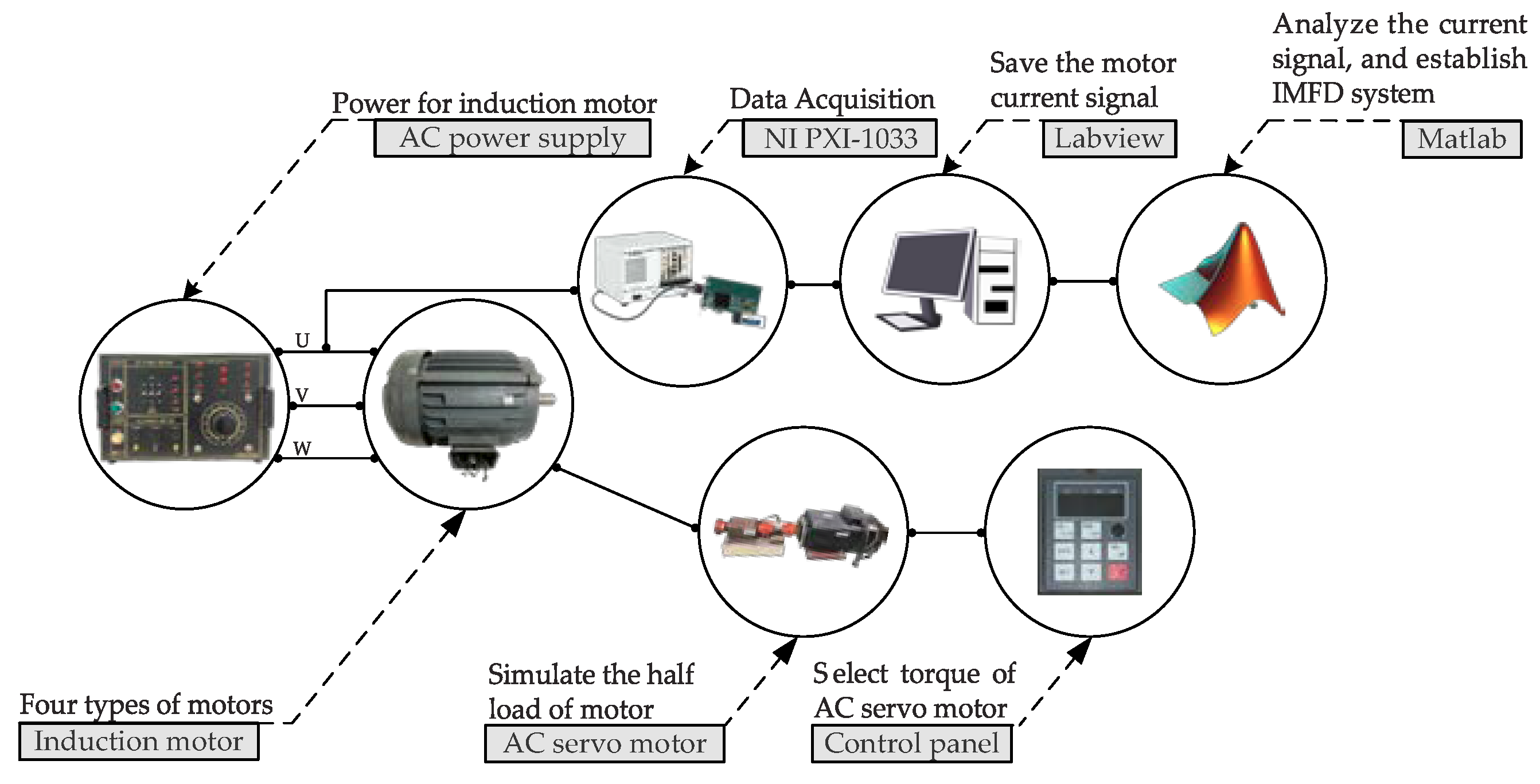
2. Measure and Analyze the Current Signals

The classes of motor faults and damages are shown in Figure 1. As the equipment layout is shown in Figure 2, this study uses the AC power supply with 3 phases and 220 volts for motors. The control panel could adjust the load of the servo motor, which has a 220 V rated voltage, a 60 Hz power frequency, a 2 Hp output, a 1764 rpm rated speed, and a 0.8 power factor. The data-acquisition equipment (PXI-1033) captures the current from all types of motors. Labview can save each observation for 2 s and save sampling frequency for 1 kHz. Corresponding to four types (one healthy motor and three faulty motors) Labview can collect 400 observations for each case, save each observation for 2 s, and save the sampling frequency at 1 kHz.

After measuring the data, this study establishes the fault-detection system with Matlab as shown in Figure 3. This classification system is divided into five parts: (a) NI PXI-1033 is used to capture 400 observations of current signals for four types of motors. The current signals will be processed by normalization, benefiting system operation. (b) A total of 1600 observations (4 classes) of normalized current signals were analyzed using MRA and HHT, while features were captured by Matlab. In this section, a fault dataset of 4 types of induction motors with 1600 observations and 4 classes is established. The number of extracted features is described in detail in the next subsection. (c) Critical features are selected by feature-selection approaches to lower the number of features. (d) In the dataset, each type is divided into 300 observations for training and 100 observations for testing. The artificial neural network is trained by the LM to build the fault-detection system. (e) Finally, the accuracy of the fault-detection system can be calculated.

2.1. MRA and Feature Distribution of Current Signals

The MRA is used to analyze the current signals of four motors. According to [38], the MRA function in (1) demonstrates that signal f(t) can be decomposed into approximation coefficient a_j and detail coefficient d_j. φ(t) is the scaling function. ψ(t) is the wavelet function, where g₀ and h₀ are filter coefficients.

$$f(t)={\displaystyle \sum _k{a}_{j0,k}{\phi }_{j0,k}(t)}+{\displaystyle \sum _j{\displaystyle \sum _k{d}_{j,k}}}{\psi }_{j,k}(t)$$

(1)

$$\phi (t)={\displaystyle \sum _k{g}_0(k)}+{\phi }_k(2t-k)$$

(2)

$$\psi (t)=\sqrt{2}{\displaystyle \sum _k{h}_0(t)}+{\phi }_k(2t-k)$$

(3)

Firstly, the MRA decomposes the signal and uses detail coefficients and approximation coefficients to compose the signal, as shown in Figure 4, where x-axis is the time and y-axis is the amplitude. Then, 60 features extracted from the signal will be composed with d1–5 and a5, as shown in

Table 1. Feature extraction of the MRA.

	a5	d5	d4	d3	d2	d1
Tmax	F1	F2	F3	F4	F5	F6
Tmin	F7	F8	F9	F10	F11	F12
Tmean	F13	F14	F15	F16	F17	F18
Tmse	F19	F20	F21	F22	F23	F24
Tstd	F25	F26	F27	F28	F29	F30
Fmax	F31	F32	F33	F34	F35	F36
Fmin	F37	F38	F39	F40	F41	F42
Fmean	F43	F44	F45	F46	F47	F48
Fmse	F49	F50	F51	F52	F53	F54
Fstd	F55	F56	F57	F58	F59	F60

, namely (1) Tmax; (2) Tmin; (3) Tmean; (4) Tmse; (5) Tstd; (6) Fmax; (7) Fmin; (8) Fmean; (9) Fmse; (10) Fstd. Features are summarily presented below. The frequency domain is analyzed with FFT. Finally, Figure 5 shows the feature distribution of IM.

(1)

Tmax: maximum of each coefficient in time domain;

(2)

Tmin: minimum of each coefficient in time domain;

(3)

Tmean: average of each coefficient in time domain;

(4)

Tmse: root mean square of each coefficient in time domain;

(5)

Tstd: standard of each coefficient in time domain;

(6)

Fmax: maximum of each coefficient in frequency domain;

(7)

Fmin: minimum of each coefficient in frequency domain;

(8)

Fmean: average of each coefficient in frequency domain;

(9)

Fmse: root mean square of each coefficient in frequency domain;

(10)

Fstd: standard of each coefficient in frequency domain.

2.2. Hilbert–Huang Transform and Feature Distribution of Current Signals

This study uses Hilbert–Huang transform (HHT) to analyze the current signals of four classes of motors. According to [39], the HHT decomposes the signal into several intrinsic mode functions (IMF) c_i by empirical mode decomposition (EMD) and calculates ${\mathit{H}}_{\mathit{i}}\left(\mathit{t}\right)$ from c_i with Hilbert transform (HT) in (4), as shown. (5) and (6) calculate the instantaneous amplitude ${\mathit{a}}_{\mathit{i}}\left(\mathit{t}\right)$ and instantaneous phase angle ${\theta }_{\mathit{i}}\left(\mathit{t}\right)$. Finally, (7) differentiates the instantaneous phase angle ${\theta }_{\mathit{i}}\left(\mathit{t}\right)$ and obtains instantaneous frequency ${\omega }_{\mathit{i}}\left(\mathit{t}\right)$.

$$H_i(t)=\frac{1}{\pi }{\displaystyle \underset{-\infty }{\overset{\infty }{\int }}\frac{c_i}{t-\tau }d\tau }$$

(4)

$$a_i(t)=\sqrt{c_i^2(t)+H_i^2(t)}$$

(5)

$${\theta }_i(t)={\tan }^{-1}\frac{H_i(t)}{c_i(t)}$$

(6)

$${\omega }_i(t)=\frac{d{\theta }_i(t)}{dt}$$

(7)

Firstly, the HHT decomposes the signal into seven (limitation of the signal) intrinsic mode functions, IMF1 (c1) to IMF7 (c7) by EMD, as shown in Figure 6, where x-axis is the amplitude, y-axis is the time. Then, instantaneous frequencies w1 to w7 are calculated with c1 to c7, as shown in Figure 7, where x-axis is the time, y-axis is the frequency. In w1, most of the bandwidths are around 60 Hz (fundamental frequency), and some of the bandwidths are close to 1 kHz, because the value of AC current emerged close to zero has a great slope. Furthermore, 70 features are extracted from c1 to c7 and w1 to w7, as shown in

Table 2. Feature extraction of the HHT.

		max	min	mean	mse	std
EMD	c1	F1	F2	F3	F4	F5
	c2	F6	F7	F8	F9	F10
	c3	F11	F12	F13	F14	F15
	c4	F16	F17	F18	F19	F20
	c5	F21	F22	F23	F24	F25
	c6	F26	F27	F28	F29	F30
	c7	F31	F32	F33	F34	F35
HT	w1	F36	F37	F38	F39	F40
	w2	F41	F42	F43	F44	F45
	w3	F46	F47	F48	F49	F50
	w4	F51	F52	F53	F54	F55
	w5	F56	F57	F58	F59	F60
	w6	F61	F62	F63	F64	F65
	w7	F66	F67	F68	F69	F70

, namely (1) max; (2) min; (3) mean; (4) mse; (5) std. Features are summarily presented below. Finally, Figure 8. shows the feature distribution of IM.

(1)

max: maximum of w1 to w7 and c1 to c7;

(2)

min: minimum of w1 to w7 and c1 to c7;

(3)

mean: average of w1 to w7 and c1 to c7;

(4)

mse: root mean square of w1 to w7 and c1 to c7;

(5)

std: standard of w1 to w7 and c1 to c7.

3. Feature-Selection Approaches for Features of the MRA and HHT

3.1. ReliefF

The ReliefF algorithm shows as Algorithm 1. ReliefF is improved for multiclass classification situations. This study uses ReliefF to calculate the correlation between feature and classification. The algorithm selects the feature $\left(F_h\right)$ from all of the features, and $F_h$ is selected as one value of the set. Then, the feature $\left(F_h\right)$ chooses the nearest values of the same classification and other classifications. In addition, function (8) is used to calculate the correlation, and features with greater correlation will be considered more important.

Algorithm 1: ReliefF

1: repeat

2:   Choose one of the features $F_h$;

3:   Choose one value $f_h$ randomly from $F_h$;

4:   Choose the nearest values $f_{nh}$ and $f_{nmb}$ with $f_h$;

5:   Calculate the $F_h$ correlation $R_{fFh}$ in (8);

6: until obtain all correlations $R_{fF}$ with ReliefF for feature selection

7: Choose the best performance of feature set for establish ANN

$$R_{fF}=W_i-(\frac{1}{km})diff(f_h,f_{nh})+(\frac{p(m\not\subset n)}{1-p(n)})(\frac{1}{km})\times diff(f_h,f_{nmb})$$

(8)

where

$$RfF \left(\begin{array}{c}{\mathit{R}}_{fF1}\\ ⋮\\ {\mathit{R}}_{fFi}\\ ⋮\\ {\mathit{R}}_{fFm}\end{array}\right),$$

is the correlation between feature and classification.

3.2. CFS

The CFS algorithm is shown as Algorithm 2. CFS calculates the Merit value for selecting the features under three conditions: (I) feature correlation and (II) correlation between feature and classification. The algorithm calculates the correlation R_f between features with Relief that is shown in (9). Next, ReliefF is used to calculate the correlation R_fF between feature and classification in (8). In addition, (III) calculates the Merit value in (10).

Algorithm 2: CFS

1: (I) The feature correlation:

2: repeat

3:   Choose two of the features $F_h$ and $F_i$;

4:   Choose one value $f_h$ randomly from $F_h$;

5:   Choose the nearest values $f_{nh}$ and $f_{nm}$ with $f_h$;

6:   Calculate the correlation between $F_h$ and $F_i$ with (9);

7: until obtain all correlation $R_F$ with Relief.

8: (II) The correlation between feature and classification:

9: Use ReliefF to calculate RfF in (8);

10: (III) Calculate the Merit value:

11: repeat

14:   Calculate the Merit value in (10);

15: until obtain the whole Merit value.

16: Choose the best performance of feature set for establish ANN.

$$R_f=W_i-(\frac{1}{k})diff{(f_h,f_{nh})}^2+(\frac{1}{k})\times diff{(f_h,f_{nm})}^2$$

(9)

where

$$Rf\left(\begin{array}{cccccc}1& {\mathit{R}}_{\mathit{f}12}& {\mathit{R}}_{\mathit{f}13}& \cdots & \cdots & {\mathit{R}}_{\mathit{f}1\mathit{m}}\\ 0& 1& {\mathit{R}}_{\mathit{f}23}& \cdots & \cdots & ⋮\\ ⋮& 0& \ddots & \cdots & {\mathit{R}}_{fhm}& ⋮\\ ⋮& 0& 0& \ddots & \cdots & ⋮\\ ⋮& ⋮& ⋮& 0& 1& ⋮\\ 0& \cdots & \cdots & \cdots & 0& 1\end{array}\right),$$

is the correlation between features;

$$\mathrm{Merit}=\frac{n_f\times {\overline{R}}_{{}_{fFi}}}{\sqrt{n_f+n_f(k-1)\times }{\overline{R}}_{{}_{fij}}}$$

(10)

3.3. CFFS

The CFFS algorithm is shown as Algorithm 3. CFFS is the feature-selection approach improved by CFS, which is proposed in our previous study [28]. CFFS selects the features under four conditions. The algorithm calculates (I) correlation between features in (9), (II) correlation between features and classification in (8), (III) Merit value in (10). Then, (IV) fitness value W_fi is calculated for Merit_new value in (11).

$$\mathrm{Merit}\_\mathrm{new}=\mathrm{Merit}\times W_{fi}$$

(11)

The fitness value was calculated by PSO. The PSO is used to optimize the weights of features [40,41] and selects the best-known solution in swarms. Therefore, this study could establish the best induction-motor fault-detection system with the features selected by CFFS and the weights of these features after training ANN.

Algorithm 3: CFFS

1: (I) The correlation between features:

2: Use Relief to calculate the correlation;

3: (II) The correlation between feature and classification:

4: Use ReliefF to calculate the correlation;

5: (III) Calculate the Merit value:

6: Use CFS to calculate the Merit value;

7: (IV) Calculate the Merit_new value:

8: repeat

9:    Select the feature set to training ANN with PSO;

10:   Calculate the fitness value Wfi from PSO;

11:   Calculate the Merit_new value in (11);

12: until obtain all the Merit_new value.

13: Choose the best performance of feature set for establish ANN.

To compare the feature-selection approach’s performance, this study chooses the 1st to the 10th feature-selection approach orders through the MRA and the HHT, which are shown in

Table 3. Features order.

Signal Processing	Feature-Selection Approach	Features Order of 1st to 10th
		1st	2nd	3rd	4th	5th	6th	7th	8th	9th	10th
MRA	ReliefF	F35	F24	F54	F60	F27	F57	F30	F21	F51	F58
	CFS	F35	F54	F60	F24	F57	F51	F58	F30	F27	F21
	CFFS	F35	F57	F58	F27	F24	F51	F60	F30	F22	F54
HHT	ReliefF	F5	F4	F61	F32	F56	F12	F40	F58	F44	F10
	CFS	F39	F40	F38	F5	F4	F13	F64	F65	F14	F45
	CFFS	F39	F5	F4	F13	F64	F43	F25	F46	F24	F45

. The MRA–ReliefF, MRA–CFS, and MRA–CFFS have the same 9 features (F35, F24, F54, F60, F27, F57, F30, F51, and F58). The HHT–ReliefF, HHT–CFS, and HHT–CFFS only have the same 2 features (F5 and F4). The important features mentioned above are marked in Figure 5 and Figure 8 (the red dot ●). Inferring to Table 3, the features extracted from the MRA with feature-selection approaches are more similar than the HHT. According to the result, the performance of feature selection is affected by the features extracted from signal processing.

4. The Result of Induction-Motor Fault Detection

This section demonstrates the results of the fault-detection system and analyzes the current signals using MRA and HHT. As shown in Figure 9, the feature-selection method is used to reduce the number of features to test the efficiency of IMFD with noise current signals (including SNR: 40 dB, 30 dB, 20 dB, and 10 dB): (a) Use Matlab to add the AWGN into current signals; (b) analyze the data; (c) select the features. The feature order after adding noise is the same as the feature-selection method applied to the original signal. (d) Training the fault-detection system. (e) Finally, obtain the accuracy of this fault-detection system. ReliefF and CFS both select features based on feature correlation, whereby the feature orders of ReliefF and CFS are the same. CFFS selects the features based on feature correlation and the performance of the fault-detection system, whereby feature orders will change every time according to accuracy. Therefore, the accuracies of the MRA–ReliefF, MRA–CFS, HHT–ReliefF, and HHT–CFS are at an average level through 50 rounds of training and testing. The MRA–CFFS and HHT–CFFS only undergo the training and testing process once, whereby the accuracy curves are more unstable than the accuracy curves of the MRA–ReliefF, MRA–CFS, HHT–ReliefF, and HHT–CFS. In conclusion, this study compares the accuracy curve of all results and proposed the best model to establish the fault-detection system.

4.1. Parameter Setting of ANN

The ANN is composed of the input layer, hidden layer, output layer, and neurons. In the hidden layer, the input is computed via weights, biases, and activation functions. The classification result is computed by the output layer. In ANN, the weight and bias of each neuron are adjusted by calculating the error between the output and the target. Updating the weights and biases during the iteration will reduce the cross-entropy loss. The parameter settings of the ANN used in this study are shown in

Table 4. Parameter setting of ANN.

Parameters	Value
Hidden layer size	10
Output layer size	4
Training ratio	75/100
Testing ratio	25/100
Training function	Levenberg-Marquardt
Learning rate	0.007
Iteration	50
Activation function	Softmax
Performance function	Cross-Entropy
Transfer function	Hyperbolic tangent sigmod

.

4.2. Compare the Signal-Processing Aproaches: The MRA, and the HHT

The accuracies of the MRA–ReliefF (Figure 10) are displayed at 60 feature numbers and the accuracies of the HHT–ReliefF (Figure 11) are displayed at 70 feature numbers under different noise conditions. The comparison results are summarized below. The accuracies under different noise conditions of the MRA–ReliefF is higher than the accuracies of the HHT–ReliefF.

(1)

In ∞ dB, MRA: 94.8%, HHT: 85.8%;

(2)

In 40 dB, MRA: 92.2%, HHT: 84.4%;

(3)

In 30 dB, MRA: 92%, HHT: 81.9%;

(4)

In 20 dB, MRA: 88.2%, HHT: 68.4%;

(5)

In 10 dB, MRA: 69.2%, HHT: 43.9%.

The accuracies of the MRA–CFS (Figure 12) are displayed at 60 feature numbers and the accuracies of the HHT–CFS (Figure 13) are displayed at 70 feature numbers under different noise conditions. The comparison results are summarized below. The accuracies under different noise conditions of the MRA–CFS are higher than the accuracy of the HHT–CFS.

(1)

In ∞ dB, MRA: 94.8%, HHT: 85.9%;

(2)

In 40 dB, MRA: 94.5%, HHT: 83.4%;

(3)

In 30 dB, MRA: 93.7%, HHT: 81.9%;

(4)

In 20 dB, MRA: 87.7%, HHT: 68%;

(5)

In 10 dB, MRA: 70.3%, HHT: 44.1%.

The accuracies of the MRA–CFFS (Figure 14) are displayed at 60 feature numbers and the accuracies of the HHT–CFFS (Figure 15) are displayed at 70 feature numbers under different noise conditions. The comparison results are summarized below. The accuracies under different noise conditions of the MRA–CFFS are higher than the accuracy of the HHT–CFFS.

(1)

In ∞ dB, MRA: 92%, HHT: 83.5%;

(2)

In 40 dB, MRA: 91.8%, HHT: 82.7%;

(3)

In 30 dB, MRA: 91.3%, HHT: 81.5%;

(4)

In 20 dB, MRA: 91%, HHT: 73.3%;

(5)

In 10 dB, MRA: 89.8%, HHT: 66%.

4.3. Compare the Feature-Selection Approaches: ReliefF, CFS, and CFFS

The highest efficiencies of the MRA with different feature-selection approaches under different noise conditions are shown in

Table 5. Result of the MRA–ReliefF.

SNR	Feature Numbers	Accuracy (%)	The Elements of the Feature Vector
∞	10	92.8	F35, F24, F54, F60, F27, F57, F30, F21, F51, F58
40	10	92.7	F35, F24, F54, F60, F27, F57, F30, F21, F51, F58
30	10	90.4	F35, F24, F54, F60, F27, F57, F30, F21, F51, F58
20	14	87.6	F35, F24, F54, F60, F27, F57, F30, F21, F51, F58, F34, F36, F28, F22
10	22	70.3	F35, F24, F54, F60, F27, F57, F30, F21, F51, F58, F34, F36, F28, F22, F52, F33, F9, F3, F49, F19, F31, F13

,

Table 6. Result of the MRA–CFS.

SNR	Feature Numbers	Accuracy (%)	The Elements of the Feature Vector
∞	7	92.02	F35, F54, F60, F24, F57, F51, F58
40	7	91.9	F35, F54, F60, F24, F57, F51, F58
30	7	90.7	F35, F54, F60, F24, F57, F51, F58
20	11	88.3	F35, F54, F60, F24, F57, F51, F58, F30, F27, F21, F52
10	20	70.3	F35, F54, F60, F24, F57, F51, F58, F30, F27, F21, F52, F34, F36, F28, F22, F33, F49, F59, F55, F31

and

Table 7. Result of the MRA–CFFS.

SNR	Feature Numbers	Accuracy (%)	The Elements of the Feature Vector
∞	3	93	F35, F57, F58
40	3	93	F35, F57, F58
30	3	93	F35, F57, F58
20	4	92.8	F35, F57, F58, F27
10	6	92	F35, F57, F58, F27, F24, F51

. The comparison is summarized as below. The accuracies of the CFFS are slightly higher than the accuracy of ReliefF and the CFS under ∞ dB, 40 dB, and 30 dB. Under severe noise conditions such as 20 dB and 10 dB, the CFFS achieves a better performance than ReliefF and the CFS.

(1)

In ∞ dB, ReliefF: 10 features and 92.8%, CFS: 7 features aFnd 92.02%, CFFS: 3 features and 93%;

(2)

In 40 dB, ReliefF: 10 features and 92.7%, CFS: 7 features and 91.9%, CFFS: 3 features and 93%;

(3)

In 30 dB, ReliefF: 10 features and 90.4%, CFS: 7 features and 90.7%, CFFS: 3 features and 93%;

(4)

In 20 dB, ReliefF: 14 features and 87.6%, CFS: 11 features and 88.3%, CFFS: 4 features and 92.8%;

(5)

In 10 dB, ReliefF: 22 features and 70.3%, CFS: 20 features and 70.3%, CFFS: 6 features and 92%.

The highest efficiencies of the HHT with different feature-selection approaches under different noise conditions are shown in

Table 8. Result of the HHT–ReliefF.

SNR	Feature Numbers	Accuracy (%)	The Elements of the Feature Vector
∞	9	78.2	F5, F4, F61, F32, F56, F12, F40, F58, F44
40	9	77.6	F5, F4, F61, F32, F56, F12, F40, F58, F44
30	9	72.9	F5, F4, F61, F32, F56, F12, F40, F58, F44
20	9	60.4	F5, F4, F61, F32, F56, F12, F40, F58, F44
10	9	43.8	F5, F4, F61, F32, F56, F12, F40, F58, F44

,

Table 9. Result of the HHT–CFS.

SNR	Feature Numbers	Accuracy (%)	The Elements of the Feature Vector
∞	13	81.3	F39, F40, F38, F5, F4, F13, F64, F65, F14, F45, F63, F15, F46
40	13	79.6	F39, F40, F38, F5, F4, F13, F64, F65, F14, F45, F63, F15, F46
30	13	75.2	F39, F40, F38, F5, F4, F13, F64, F65, F14, F45, F63, F15, F46
20	13	62.9	F39, F40, F38, F5, F4, F13, F64, F65, F14, F45, F63, F15, F46
10	13	44.6	F39, F40, F38, F5, F4, F13, F64, F65, F14, F45, F63, F15, F46

and

Table 10. Result of the HHT–CFFS.

SNR	Feature Numbers	Accuracy (%)	The Elements of the feature Vector
∞	7	74.8	F39, F5, F4, F13, F64, F43, F25
40	6	73.5	F39, F5, F4, F13, F64, F43
30	6	73	F39, F5, F4, F13, F64, F43
20	6	72.3	F39, F5, F4, F13, F64, F43
10	6	71.5	F39, F5, F4, F13, F64, F43

. The comparison is summarized below. The accuracies of the CFFS are slightly lower than the accuracy of ReliefF and the CFS under ∞ dB, 40 dB, and 30 dB. Under severe noise conditions such as 20 dB and 10 dB, the CFFS achieves a better performance than ReliefF and the CFS.

(1)

In ∞ dB, ReliefF: 9 features and 78.2%, CFS: 13 feature and 81.3%, CFFS: 7 features and 74.8%;

(2)

In 40 dB, ReliefF: 9 features and 77.6%, CFS: 13 features and 79.6%, CFFS: 6 features and 73.5%;

(3)

In 30 dB, ReliefF: 9 features and 72.9%, CFS: 13 features and 75.2%, CFFS: 6 features and 73%;

(4)

In 20 dB, ReliefF: 9 features and 60.4%, CFS: 13 features and 62.9%, CFFS: 6 features and 72.3%;

(5)

In 10 dB, ReliefF: 9 features and 43.8%, CFS: 13 features and 44.6%, CFFS: 6 features and 71.5%.

According to the comparison of the signal-processing approaches and feature-selection approaches, the performance of the MRA is better than the HHT, and the CFFS can establish an effective fault-detection system than ReliefF and CFS. The result could be inferred by the feature distribution of MRA (Figure 5) and the HHT (Figure 8). The features of MRA (Figure 5) have more significant features than the HHT (Figure 8). For establishing the fault-detection system, the selected signal-processing approach has an impact on the system, and the system established with the feature-selection approach could reduce the considerable feature numbers.

5. Conclusions

The study proposes the CFFS with the advantage of filter and wrapper; therefore, the CFFS has significant performance in the fault-detection system. According to the results of this research, the choice of signal processing and feature-selection approach is a crucial influence on the accuracy of the fault-detection system. MRA is one useful method to analyze the faulty motor in this paper, which provides good features for the CFFS, which has a significant effect on the system, reducing 57 (95%) of the features from MRA and achieving 93% accuracy. The system established with CFFS also achieves excellent performance under 40 to 10 dB AWGN, reducing about 54 to 57 (90% to 95%) features and maintaining an accuracy of about 92% to 93%. In this research, the low-dimensional feature is suitable to use CFFS. In other words, CFFS uses in other cases with high-dimensional features could have higher operating costs; this factor is the limitation for CFFS. Therefore, this study establishes the fault-detection system with MRA and CFFS for the faulty motors in this study.

References

1. Zhang, P.; Shu, S.; Zhou, M. An online fault detection model and strategies based on SVM-grid in clouds. IEEE/CAA J. Autom. Sin. 2018, 5, 445–456. [Google Scholar] [CrossRef]
2. Wang, H.; Lu, S.; Qian, G.; Ding, J.; Liu, Y.; Wang, Q. A two-step strategy for online fault detection of high-resistance connection in BLDC motor. IEEE Trans. Power Electron. 2020, 35, 3043–3053. [Google Scholar] [CrossRef]
3. Mao, W.; Chen, J.; Liang, X.; Zhang, X. A new online detection approach for rolling bearing incipient fault via self-adaptive deep feature matching. IEEE Trans. Instrum. Meas. 2019, 69, 443–456. [Google Scholar] [CrossRef]
4. Antonino-Daviu, J.; Aviyente, S.; Strangas, E.G.; Riera-Guasp, M. Scale invariant feature extraction algorithm for the automatic diagnosis of rotor asymmetries in induction motors. IEEE Trans. Ind. Inform. 2013, 9, 100–108. [Google Scholar] [CrossRef]
5. Bazurto, A.J.; Quispe, E.C.; Mendoza, R.C. Causes and failures classification of industrial electric motor. In Proceedings of the 2016 IEEE Andescon, Arequipa, Peru, 19–21 October 2016; pp. 1–4. [Google Scholar]
6. Rodriguez-Donate, C.; Romero-Troncoso, R.J.; Garcia-Perez, A.; Razo-Montes, D.A. FPGA based embedded system for induction motor failure monitoring at the start-up transient vibrations with wavelets. IEEE Trans. Instrum. Meas. 2010, 59, 63–72. [Google Scholar]
7. Romero-Troncoso, R. Multirate signal processing to improve FFT-based analysis for detecting faults in induction motors. IEEE Trans. Ind. Electron. 2016, 13, 1291–1300. [Google Scholar] [CrossRef]
8. Riera-Guasp, M.; Pineda-Sanchez, M.; Pérez-Cruz, J.; Puche-Panadero, R.; Roger-Folch, J.; Antonino-Daviu, J.A. Diagnosis of induction motor faults via Gabor analysis of the current in transient regime. IEEE Trans. Instrum. Meas. 2012, 61, 1583–1596. [Google Scholar] [CrossRef]
9. Climente-Alarcon, V.; Antonino-Daviu, J.A.; Haavisto, A.; Arkkio, A. Diagnosis of induction motors under varying speed operation by principal slot harmonic tracking. IEEE Trans. Ind. Appl. 2015, 51, 3591–3599. [Google Scholar] [CrossRef] [Green Version]
10. Ali, M.Z.; Liang, X. Threshold-based induction motors single- and multifaults diagnosis using discrete wavelet transform and measured stator current signal. Can. J. Electr. Comput. Eng. 2020, 43, 136–145. [Google Scholar] [CrossRef]
11. Fan, H.; Shao, S.; Zhang, X.; Wan, X.; Cao, X.; Ma, H. Intelligent fault diagnosis of rolling bearing using FCM clustering of EMD-PWVD vibration images. IEEE Access 2020, 8, 45194–145206. [Google Scholar] [CrossRef]
12. Huo, Z.; Zhang, Y.; Francq, P.; Shu, L.; Huang, J. Incipient fault diagnosis of roller bearing using optimized wavelet transform based multi-speed vibration signatures. IEEE Access 2017, 5, 19442–19456. [Google Scholar] [CrossRef] [Green Version]
13. Trujillo-Guajardo, L.A.; Rodriguez-Maldonado, J.; Moonem, M.A.; Platas-Garza, M.A. A multiresolution Taylor–Kalman approach for broken rotor bar detection in cage induction motors. IEEE Trans. Instrum. Meas. 2018, 67, 1317–1328. [Google Scholar] [CrossRef]
14. Rabbi, S.F.; Little, M.L.; Saleh, S.A.; Rahman, M.A. A novel technique using multiresolution wavelet packet decomposition for real time diagnosis of hunting in line start IPM motor drives. IEEE Trans. Ind. Appl. 2017, 53, 3005–3019. [Google Scholar] [CrossRef]
15. Mishra, M.; Rout, P.K. Detection and classification of micro-grid faults based on HHT and machine learning techniques. IET Gener. Transm. Distrib. 2017, 12, 388–397. [Google Scholar] [CrossRef]
16. Alvarez-Gonzalez, F.; Griffo, A.; Wang, B. Permanent magnet synchronous machine stator windings fault detection by Hilbert-Huang transform. In Proceedings of the International Conference on Power Electronics, Machines and Drives, Liverpool, UK, 17–19 April 2018; pp. 3505–3509. [Google Scholar]
17. Esfahani, E.T.; Wang, S.; Sundararajan, V. Multisensor wireless system for eccentricity and bearing fault detection in induction motors. IEEE/ASME Trans. Mech. 2014, 19, 818–826. [Google Scholar] [CrossRef]
18. Espinosa, A.G.; Rosero, J.A.; Cusido, J.; Romeral, L.; Ortega, J.A. Fault detection by means of Hilbert–Huang transform of the stator current in a PMSM with demagnetization. IEEE Trans. Energy Convers. 2010, 25, 312–318. [Google Scholar] [CrossRef] [Green Version]
19. Oyamada, M. Extracting feature engineering knowledge from data science notebooks. In Proceedings of the IEEE International Conference on Big Data (Big Data), Los Angeles, CA, USA, 9–12 December 2019. [Google Scholar]
20. Al-Otaibi, R.; Jin, N.; Wilcox, T.; Flach, P. Feature construction and calibration for clustering daily load curves from smart-meter data. IEEE Trans. Ind. Inform. 2016, 12, 6452–6654. [Google Scholar] [CrossRef] [Green Version]
21. Neshatian, K.; Zhang, M.; Andreae, P. A filter approach to multiple feature construction for symbolic learning classifiers using genetic programming. IEEE Trans. Evol. Comput. 2012, 16, 645–661. [Google Scholar] [CrossRef]
22. Imani, M.; Ghassemian, H. Band clustering-based feature extraction for classification of hyperspectral images using limited training samples. IEEE Geosci. Remote Sens. Lett. 2014, 11, 1325–1329. [Google Scholar] [CrossRef]
23. Godse, R.; Bhat, S. Mathematical morphology-based feature-extraction technique for detection and classification of faults on power transmission line. IEEE Access 2020, 8, 38459–38471. [Google Scholar] [CrossRef]
24. Yang, H.; Meng, C.; Wang, C. Data-driven feature extraction for analog circuit fault diagnosis using 1-D convolutional neural network. IEEE Access 2020, 8, 18305–18315. [Google Scholar] [CrossRef]
25. Panigrahy, P.S.; Santra, D.; Chattopadhyay, P. Feature engineering in fault diagnosis of induction motor. In Proceedings of the 2017 3rd International Conference on Condition Assessment Techniques in Electrical Systems (CATCON), Rupnagar, India, 16–18 November 2017. [Google Scholar]
26. Rauber, T.W.; de Assis Boldt, F.; Varejão, F.M. Heterogeneous feature models and feature selection applied to bearing fault diagnosis. IEEE Trans. Ind. Electron. 2015, 62, 637–646. [Google Scholar] [CrossRef]
27. Van, M.; Kang, H.J. Bearing-fault diagnosis using non-local means algorithm and empirical mode decomposition-based feature extraction and two-stage feature selection. Sci. Meas. Technol. 2015, 9, 671–680. [Google Scholar] [CrossRef]
28. Lee, C.Y.; Wen, M.S. Establish induction motor fault diagnosis system based on feature selection approaches with MRA. Processes 2020, 8, 1055. [Google Scholar] [CrossRef]
29. Hu, B.; Li, X.; Sun, S.; Ratcliffe, M. Attention recognition in EEG-based affective learning research using CFS+KNN algorithm. IEEE/ACM Trans. Comput. Biol. Bioinform. 2018, 15, 38–45. [Google Scholar] [CrossRef]
30. Fu, R.; Wang, P.; Gao, Y.; Hua, X. A new feature selection method based on Relief and SVM-RFE. In Proceedings of the 2014 12th International Conference on Signal Processing (ICSP), Hangzhou, China, 19–23 October 2014. [Google Scholar]
31. Fu, R.; Wang, P.; Gao, Y.; Hua, X. A combination of relief feature selection and fuzzy k-nearest neighbor for plant species identification. In Proceedings of the 2016 International Conference on Advanced Computer Science and Information Systems (ICACSIS), Malang, Indonesia, 15–16 October 2016. [Google Scholar]
32. Huang, Z.; Yang, C.; Zhou, X.; Huang, T. A hybrid feature selection method based on binary state transition algorithm and ReliefF. IEEE J. Biomed. Health Inform. 2019, 23, 1888–1898. [Google Scholar] [CrossRef]
33. Singh, A.; Thakur, N.; Sharma, A. A review of supervised machine learning algorithms. In Proceedings of the 2016 3rd International Conference on Computing for Sustainable Global Development (INDIACom), New Delhi, India, 16–18 March 2016; pp. 1310–1315. [Google Scholar]
34. Wilamowski, B.M.; Yu, H. Improved computation for Levenberg-Marquardt training. IEEE Trans. Neural Netw. 2010, 21, 930–937. [Google Scholar] [CrossRef]
35. Fu, X.; Li, S.; Fairbank, M.; Wunsch, D.C.; Alonso, E. Training recurrent neural networks with the Levenberg—Marquardt Algorithm for optimal control of a grid-connected converter. IEEE Trans. Neural Netw. Learn. Syst. 2014, 26, 1900–1912. [Google Scholar] [CrossRef] [Green Version]
36. Lv, C.; Xing, Y.; Zhang, J.; Na, X.; Li, Y.; Liu, T.; Cao, D.; Wang, F.-Y. Levenberg–Marquardt backpropagation training of multilayer neural networks for state estimation of a safety-critical cyber-physical system. IEEE Trans. Ind. Inform. 2018, 14, 3436–3446. [Google Scholar] [CrossRef] [Green Version]
37. Ngia, L.S.H.; Sjoberg, J. Efficient training of neural nets for nonlinear adaptive filtering using a recursive Levenberg–Marquardt algorithm. IEEE Trans. Signal Process. 2000, 48, 1915–1927. [Google Scholar] [CrossRef]
38. Mallat, G. A theory for multi-resolution signal decomposition (The wavelet representation). IEEE Trans. Pattern Anal. Mach. Intell. 1989, PAMI-11, 674–693. [Google Scholar] [CrossRef] [Green Version]
39. Yi, L.; Hao, A.; Shuangshuang, B. Hilbert-Huang transform and the application. In Proceedings of the 2020 IEEE International Conference on Artificial Intelligence and Information Systems (ICAIIS), Dalian, China, 20–22 March 2020; pp. 534–539. [Google Scholar]
40. Lee, C.Y.; Tuegeh, M. An optimal solution for smooth and non-smooth cost functions-based economic dispatch problem. Energies 2020, 13, 3721. [Google Scholar] [CrossRef]
41. Fernández-Martínez, J.L.; García-Gonzalo, E. Stochastic stability analysis of the linear continuous and discrete PSO models. IEEE Trans. Evol. Comput. 2011, 15, 405–423. [Google Scholar] [CrossRef]
Figure 1. Faulty motor failure sample. (a) Bearing fault (0.53 mm width and 1.96 mm length), (b) interturn short circuit (5 insulation destructive coils), (c) broken rotor bar (2 holes—10 mm depth and 8 mm diameter).
Mathematics 10 02250 g001
Figure 2. Equipment layout.
Mathematics 10 02250 g002
Figure 3. Schematic diagram of classification system. (a) capture the observations, (b) build fault detection dataset, (c) feature selection, (d) train the ANN, (e) classification result.
Mathematics 10 02250 g003
Figure 4. The MRA of current signal. (a) Normal motor, (b) bearing fault, (c) interturn short circuit, (d) broken rotor bar.
Mathematics 10 02250 g004
Figure 5. Feature distribution of the MRA. (a) Normal motor, (b) bearing fault, (c) interturn short circuit, (d) broken rotor bar.
Mathematics 10 02250 g005
Figure 6. The EMD of current signal. (a) Normal motor, (b) bearing fault, (c) interturn short circuit, (d) broken rotor bar.
Mathematics 10 02250 g006
Figure 7. Instantaneous frequency of EMD. (a) Normal motor, (b) bearing fault, (c) interturn short circuit, (d) broken rotor bar.
Mathematics 10 02250 g007
Figure 8. Feature distribution of the HHT. (a) Normal motor, (b) bearing fault, (c) interturn short circuit, (d) broken rotor bar.
Mathematics 10 02250 g008
Figure 9. Schematic diagram of current signal added the noise to establish fault-detection system. (a) capture the observations, (b) build fault detection dataset, (c) feature selection, (d) train the ANN, (e) classification result.
Mathematics 10 02250 g009
Figure 10. Accuracy curves of the MRA–ReliefF.
Mathematics 10 02250 g010
Figure 11. Accuracy curves of the HHT–ReliefF.
Mathematics 10 02250 g011
Figure 12. Accuracy curves of the MRA–CFS.
Mathematics 10 02250 g012
Figure 13. Accuracy curves of the HHT–CFS.
Mathematics 10 02250 g013
Figure 14. Accuracy curves of the MRA–CFFS.
Mathematics 10 02250 g014
Figure 15. Accuracy curves of the HHT–CFFS.
Mathematics 10 02250 g015