A Robust Single-Machine Scheduling Problem with Two Job Parameter Scenarios

Abstract

In many real-world environments, machine breakdowns or worker performance instabilities cause uncertainty in job processing times, while working environment changes or transportation delays will postpone finished production for customers. The factors that impact the task processing times and/or deadlines vary. In view of the uncertainty, job processing times and/or job due dates cannot be fixed numbers. Inspired by this fact, we introduce a scenario-dependent processing time and due date concept into a single-machine environment. The measurement minimizes the total job tardiness in the worst case. The same problem without the presence of processing time uncertainty has been an NP-hard problem. First, to solve this difficult model, an exact method, including a lower bound and some dominance properties, is proposed. Next, three scenario-dependent heuristic algorithms are proposed. Additionally, a population-based iterated greedy algorithm is proposed in the hope of increasing the diversity of the solutions. The results of all related algorithms are determined and compared using the appropriate statistical tools.

1. Introduction

The operational parameters of a scheduling problem cannot be fixed or predetermined. For example, the processing time might be influenced by machine breakdowns or altered by the number of ordered items (products), the release date might be delayed by unexpected factors, and the due date might have to be adjusted earlier/later for customers. Therefore, these parameters in a scheduling problem can be treated as uncertain. For example, the travel time of a caregiver might vary and the service time of an elder could be prolonged in the home health industry. In home healthcare situations, assigning caregivers and routes of services is a practical and important issue. For example, [1] supplied a framework to make a robust scheduling problem for an institution. Other examples were presented in the facility location problem by [2], in the discrete time/cost trade-off problem by [3], and in random quality deteriorating hybrid manufacturing by [4].

To address these situations, researchers attempt to search job sequences or job schedules to reduce the risk or to minimize one or several aspects of loss measures. This led to the robust approach to solve a scheduling model with scenario-dependent effects [5,6]. There were two deterministic methods (in contrast to stochastic methods) to model the uncertain parameters of a scheduling problem discussed in the relevant literature. The uncertain parameters were either bounded within an interval (continuous case) or described by a finite number of scenarios (discrete case) [5,6]. The discrete scenario robust scheduling problem was first studied by [6]. Taking a finite number of scenarios into consideration, they discussed three robust measures in a single-machine setting, i.e., the absolute robust, the robust deviation, and the relative robust deviation [7]. The main objective function is to seek an optimal job schedule among all possible permutations over all possible scenarios. Other studies pertinent to machine scheduling in the face of uncertainty for discrete cases include [8,9]. Additionally, some recent distributionally robust optimization scheduling problems with uncertain processing times or due dates include [10,11].

The total tardiness measure is very important in practice. Tardiness relates to backlog (of order) issues, which may cause customers to demand compensation for delays and loss of credit. In addition to the single-machine operation environment, the total tardiness minimization has been investigated in other work environments, e.g., flow-shop, job shop, parallel, and order scheduling problems (refer to [12,13], respectively). Readers can refer to the review papers by [14,15] on the total (weighted) tardiness criterion in the scheduling area. More recently, [16] introduced the scenario-dependent idea into a parallel-machine order scheduling problem where the tardiness criterion is minimized.

However, the performance measure total tardiness together with the uncertainty of parameters is rarely discussed in the literature for deterministic models of scheduling problems. Moreover, [17] noted that “single-machine models often have properties that have neither machines in parallel nor machines in series. The results that can be obtained for single machine models not only provide insights into a single machine environment, they also provide a basis for heuristics that are applicable to more complicated machine environments…” (see page 35 in [17]). Therefore, we introduce scenario-dependent due dates and scenario-dependent processing times to a single-machine setting, in which the criterion is the sum of tardiness of all given jobs.

This work provides several contributions: We introduce a scenario-dependent processing time and due date concept to a single-machine scheduling problem to minimize the sum of job tardiness in the worst case. We derive a lower bound and several properties to increase the power capability of a branch-and-bound (B&B) method for an exact solution. In addition, we propose three different values for a parameter in one local search heuristic method and a population-based iterative greedy algorithm for near-optimal solutions. The organization of this article is as follows: Section 2 states the formulation of the investigated problem. Section 3 derives one lower bound and eight dominances used in the B&B method, introduces three different values for a parameter in one local search heuristic method and a population-based iterative greedy (PBIG) method, and proposes details of the branch-and-bound method. Section 4 presents tuning parameters in the iterative greedy algorithm. Section 5 reports and analyses the related simulation results. The conclusions and suggestions are summarized in Section 6.

2. Problem Statement

In this section, the study under consideration is formally described. There is a set J of n jobs {J₁, J₂, …, J_n} to be processed on a single-machine environment. The machine can execute at most one job at a time, preemption is not allowed, and their ready times are zero. Another assumption is that there are two scenarios of job parameters (due dates and processing times) to capture the uncertainty of the two parameters discretely. Assume that $t_j^{\left(v\right)}$ represents the processing time while $d_j^{\left(v\right)}$ represents the due date of job $J_j$ for scenario v = 1, 2. Furthermore, for scenario v, let $C_j^{\left(\nu \right)}\left(\mathsf{\sigma }\right)$ represent the completion time of job $J_j$, where $\mathsf{\sigma }$ is a job sequence (schedule). The tardiness of $J_j$ is defined to be $T_j^{\left(\upsilon \right)}\left(\sigma \right)=\max \left\{0, C_j^{\left(\nu \right)}\left(\sigma \right)-d_j^{\left(v\right)}\right\}$, and the total tardiness for all n jobs is $\sum T_j^{\left(\upsilon \right)}\left(\sigma \right)$ for scenario v. Without considering the uncertainty of the parameters, the classic tardiness minimization scheduling problem in a single-machine environment, denoted by $1\left|\right|\sum T_j\left(\sigma \right)$, has been shown to be an NP-hard problem. Accordingly, the considered problem can be denoted by $\underset{\sigma }{\mathrm{MIN}}\underset{\nu }{\mathrm{MAX}}(1||\sum T_j^{\left(\upsilon \right)}\left(\sigma \right), t_j^{\left(\upsilon \right)})$ and as an NP-hard problem ([18,19]) That is, under the assumptions that $t_j^{\left(v\right)}$ and $d_j^{\left(v\right)}$ are uncertain and can be captured discretely by scenario v = 1, 2, we are required to find an optimal robust schedule ${\sigma }^{\ast }$ such that ${\sigma }^{\ast }\in \arg \underset{\sigma \in all permutations}{\min }\left\{\underset{\nu =1,2}{\max }{{\displaystyle \sum }}_{j=1}^n{T}_j^{\nu }\left(\sigma \right)\right\}$. In other words, the aim of this study is to seek a robust single-machine schedule incorporating scenario-dependent due dates and scenario-dependent processing times in which the tardiness measurement for the worst scenario can be minimized (optimal).

3. Heuristics and Branch-and-Bound Method

In this section, we derive some properties and a lower bound to use in the branch- and-bound method, develop three different values for a parameter in one local search heuristic method, and provide a population-based iterative greedy (PBIG) algorithm.

3.1. Properties

In this section, nine properties and one lower bound will be built with the purpose of aiding the search for optimal robust solutions quickly in a branch-and-bound method ([20,21,22]). Let ${\sigma }_1=\left(\delta ,i,j,{\delta }^{\prime }\right)$ and ${\sigma }_2=\left(\delta ,j,i,{\delta }^{\prime }\right)$ present two full schedules, where $\delta$ and ${\delta }^{\prime }$ denote two partial sequences. To conclude that ${\sigma }_1$ dominates ${\sigma }_2$, the following suffices:

$${max}_{v=1,2}\left\{T_i^{\left(v\right)}\left({\sigma }_1\right)+T_j^{\left(v\right)}\left({\sigma }_1\right)\right\}<{max}_{v=1,2}\left\{T_j^{\left(v\right)}\left({\sigma }_2\right)+T_i^{\left(v\right)}\left({\sigma }_2\right)\right\},$$

and

$$C_j^{\left(v\right)}\left({\sigma }_1\right)\le C_i^{\left(v\right)}\left({\sigma }_2\right), v=1, 2.$$

In addition, for scenario $\nu$, let $s^{\left(\upsilon \right)}$ denote the starting time of job i and the starting time of job j in the subsequence $\delta$, of ${\sigma }_1$ and ${\sigma }_2$. The details for proving Properties 2–9 are similar to those of Property 1; thus, only the proof for Property 1 is given here.

Property 1.

If$s^{\left(1\right)}+t_i^{\left(1\right)}+t_j^{\left(1\right)}<d_j^{\left(1\right)}$,$s^{\left(2\right)}+t_i^{\left(2\right)}+t_j^{\left(2\right)}<min\left\{d_j^{\left(2\right)},d_i^{\left(2\right)}\right\}$, and$s^{\left(1\right)}+t_i^{\left(1\right)}<d_i^{\left(1\right)}$<$s^{\left(1\right)}+t_i^{\left(1\right)}+t_j^{\left(1\right)}$, then${\sigma }_1$dominates${\sigma }_2$.

Proof. 

In the following, we compute the total tardiness of sequence ${\sigma }_1$ and sequence ${\sigma }_2$. The desired results are obtained.

By the definition of tardiness, for the sequence ${\sigma }_1$, the following are easily seen:

$$T_i^{\left(1\right)}\left({\sigma }_1\right)=max\left\{0, C_i^{\left(1\right)}\left({\sigma }_1\right)-d_i^{\left(1\right)}\right\}=max\left\{0, \left(s^{\left(1\right)}+t_i^{\left(1\right)}\right)-d_i^{\left(1\right)}\right\},$$

$$T_j^{\left(1\right)}\left({\sigma }_1\right)=max\left\{0, C_j^{\left(1\right)}\left({\sigma }_1\right)-d_j^{\left(1\right)}\right\}=max\left\{0, \left(s^{\left(1\right)}+t_i^{\left(1\right)}+t_j^{\left(1\right)}\right)-d_j^{\left(1\right)}\right\}.$$

Now, the given conditions $s^{\left(1\right)}+t_i^{\left(1\right)}<d_i^{\left(1\right)}$ and $s^{\left(1\right)}+t_i^{\left(1\right)}+t_j^{\left(1\right)}<d_j^{\left(1\right)}$ imply that

$$T_i^{\left(1\right)}\left({\sigma }_1\right)=0 \mathrm{and} T_j^{\left(1\right)}\left({\sigma }_1\right)=0, \mathrm{respectively}.$$

(1)

$$T_i^{\left(2\right)}\left({\sigma }_1\right)=max\left\{0, C_i^{\left(2\right)}\left({\sigma }_1\right)-d_i^{\left(2\right)}\right\}=max\left\{0, \left(s^{\left(2\right)}+t_i^{\left(2\right)}\right)-d_i^{\left(2\right)}\right\},$$

$T_j^{\left(2\right)}\left({\sigma }_1\right)=max\left\{0, C_j^{\left(2\right)}\left({\sigma }_1\right)-d_j^{\left(2\right)}\right\}=max\left\{0, \left(s^{\left(2\right)}+t_i^{\left(2\right)}+t_j^{\left(2\right)}\right)-d_j^{\left(2\right)}\right\}$. From the given condition $s^{\left(2\right)}+t_i^{\left(2\right)}+t_j^{\left(2\right)}<\min \left\{d_i^{\left(2\right)}, d_j^{\left(2\right)}\right\}$, then

$$T_i^{\left(2\right)}\left({\sigma }_1\right)=0=T_j^{\left(2\right)}\left({\sigma }_1\right).$$

(2)

Similarly, for the sequence ${\sigma }_2$, the given condition $s^{\left(1\right)}+t_i^{\left(1\right)}+t_j^{\left(1\right)}<d_j^{\left(1\right)}$ implies that

$$T_j^{\left(1\right)}\left({\sigma }_2\right)=max\left\{0, C_j^{\left(1\right)}\left({\sigma }_2\right)-d_j^{\left(1\right)}\right\}=max\left\{0, \left(s^{\left(1\right)}+t_j^{\left(1\right)}\right)-d_j^{\left(1\right)}\right\}=0.$$

(3)

The given condition $d_i^{\left(1\right)}<s^{\left(1\right)}+t_i^{\left(1\right)}+t_j^{\left(1\right)}$ implies that

$$T_i^{\left(1\right)}\left({\sigma }_2\right)=max\left\{C_i^{\left(1\right)}\left({\sigma }_2\right)-d_i^{\left(1\right)},0\right\}=max\left\{\left(s^{\left(1\right)}+t_j^{\left(1\right)}+t_i^{\left(1\right)}\right)-d_i^{\left(1\right)},0\right\}=\left[s^{\left(1\right)}+t_i^{\left(1\right)}+t_j^{\left(1\right)}-d_i^{\left(1\right)}\right]>0.$$

(4)

Thus, combining Equations (1) through (4), the desired inequality is the following:

$${max}_{v=1,2}\left\{T_i^{\left(v\right)}\left({\sigma }_1\right)+T_j^{\left(v\right)}\left({\sigma }_1\right)\right\}=0<{max}_{v=1,2}\left\{T_j^{\left(v\right)}\left({\sigma }_2\right)+T_i^{\left(v\right)}\left({\sigma }_2\right)\right\}=\left[s^{\left(1\right)}+t_i^{\left(1\right)}+t_j^{\left(1\right)}-d_i^{\left(1\right)}\right].\square$$

Property 2.

If$d_j^{\left(2\right)}>s^{\left(2\right)}+t_i^{\left(2\right)}+t_j^{\left(2\right)}$,$s^{\left(1\right)}+t_i^{\left(1\right)}+t_j^{\left(1\right)}<min\left\{d_j^{\left(1\right)},d_i^{\left(1\right)}\right\}$, and$s^{\left(2\right)}+t_i^{\left(2\right)}+t_j^{\left(2\right)}>d_i^{\left(2\right)}>s^{\left(2\right)}+t_i^{\left(2\right)}$, then${\sigma }_1$dominates${\sigma }_2$.

Property 3.

If$s^{\left(2\right)}+t_i^{\left(2\right)}+t_j^{\left(2\right)}<min\left\{d_j^{\left(2\right)},d_i^{\left(2\right)}\right\}$,$d_i^{\left(1\right)}$<$s^{\left(1\right)}+t_i^{\left(1\right)}$, and$s^{\left(1\right)}+t_i^{\left(1\right)}+t_j^{\left(1\right)}<d_j^{\left(1\right)}$, then${\sigma }_1$dominates${\sigma }_2$.

Property 4.

If$d_i^{\left(2\right)}$<$s^{\left(2\right)}+t_i^{\left(2\right)}$,$s^{\left(1\right)}+t_i^{\left(1\right)}+t_j^{\left(1\right)}<min\left\{d_j^{\left(1\right)},d_i^{\left(1\right)}\right\}$, and$s^{\left(2\right)}+t_i^{\left(2\right)}+t_j^{\left(2\right)}<d_j^{\left(2\right)}$, then${\sigma }_1$dominates${\sigma }_2$.

Property 5.

If$d_i^{\left(1\right)}$<$d_j^{\left(1\right)}$,$t_i^{\left(1\right)}<t_j^{\left(1\right)}$, and$s^{\left(2\right)}+t_i^{\left(2\right)}+t_j^{\left(2\right)}<min\left\{d_j^{\left(2\right)},d_i^{\left(2\right)}\right\}$, then${\sigma }_1$dominates${\sigma }_2$.

Property 6.

If$d_i^{\left(2\right)}$<$d_j^{\left(2\right)}$,$s^{\left(1\right)}+t_i^{\left(1\right)}+t_j^{\left(1\right)}<min\left\{d_j^{\left(1\right)},d_i^{\left(1\right)}\right\}$, and$t_i^{\left(2\right)}<t_j^{\left(2\right)}$, then${\sigma }_1$dominates${\sigma }_2$.

Property 7.

If$t_i^{\left(2\right)}<t_j^{\left(2\right)}$,$s^{\left(1\right)}+t_j^{\left(1\right)}<d_j^{\left(1\right)}$,$d_i^{\left(2\right)}<s^{\left(2\right)}+t_i^{\left(2\right)}$,$d_j^{\left(2\right)}<s^{\left(2\right)}+t_j^{\left(2\right)}$, and$s^{\left(1\right)}+t_i^{\left(1\right)}<d_i^{\left(1\right)}$<$s^{\left(1\right)}+t_j^{\left(1\right)}$, then${\sigma }_1$dominates${\sigma }_2$.

Property 8.

If$t_i^{\left(1\right)}<t_j^{\left(1\right)}$,$s^{\left(2\right)}+t_j^{\left(2\right)}<d_j^{\left(2\right)}$,$d_i^{\left(1\right)}<s^{\left(1\right)}+t_i^{\left(1\right)}$,$d_j^{\left(1\right)}<s^{\left(1\right)}+t_j^{\left(1\right)}$, and$s^{\left(2\right)}+t_i^{\left(2\right)}<d_i^{\left(2\right)}$<$s^{\left(2\right)}+t_j^{\left(2\right)}$, then${\sigma }_1$dominates${\sigma }_2$.

Property 9.

If$\forall$s = 1, 2,$t_i^{\left(s\right)}<t_j^{\left(s\right)}$, and$d_i^{\left(s\right)}<d_j^{\left(s\right)}$, then${\sigma }_1$dominates${\sigma }_2$.

3.2. A Lower Bound

Continuing the results of the dominance rules, the searching power of the B&B method is closely related to a lower bound to cut branching nodes. Next, we will introduce a simple lower bound for use in the B&B method. Let $\mathsf{\sigma }=\left\{J_{\left[1\right]},J_{\left[2\right]},\cdots ,J_{\left[k\right]},US\right\}$ be a schedule where the US denotes q (=n-k) unscheduled jobs under scenario v = 1, 2. Following the definition of the completion times in US, we have the following:

$$C_{\left[k+l\right]}^{\left(s\right)}\left(\mathrm{US}\right)=s^{\left(s\right)}+{{\displaystyle \sum }}_{i=1}^l{t}_{\left[k+i\right]}^{\left(s\right)}, l=1, \dots , q; s=1, 2.$$

The total tardiness of an active node can be obtained for the unscheduled k+l jobs under scenario v = 1, 2 and is the following:

$$T_{\left[k+l\right]}^{\left(v\right)}\left(\mathrm{US}\right)=\max \left\{s^{\left(v\right)}+{{\displaystyle \sum }}_{i=1}^l{t}_{\left(k+i\right)}^{\left(v\right)}-d_{\left(k+l\right)}^{\left(v\right)}, 0\right\}, l=1, \dots , q; v=1, 2.$$

where $t_{\left(k+1\right)}^{\left(v\right)}\le \dots \le t_{\left(k+q\right)}^{\left(v\right)}$ are increasing sequences of $t_{k+1}^{\left(v\right)},\dots , t_{k+q}^{\left(v\right)}$ and $d_{\left(k+1\right)}^{\left(v\right)}\le \dots \le d_{\left(k+q\right)}^{\left(v\right)}$ are increasing sequences of $d_{k+1}^{\left(1\right)},\dots , d_{k+q}^{\left(1\right)}$, v = 1, 2. Let AS =$\left\{J_{\left[1\right]},J_{\left[2\right]},\cdots ,J_{\left[k\right]}\right\}$; thus, we obtain the following lower bound:

$$\mathrm{Lower} \mathrm{bound}=({{\displaystyle \sum }}_{i=1}^k{T}_{\left[i\right]}^{\left(1\right)}\left(\mathrm{AS}\right)+{{\displaystyle \sum }}_{i=k+1}^q{T}_{\left[i\right]}^{\left(1\right)}\left(\mathrm{US}\right)+{{\displaystyle \sum }}_{i=1}^k{T}_{\left[i\right]}^{\left(2\right)}\left(\mathrm{AS}\right)+{{\displaystyle \sum }}_{i=k+1}^q{T}_{\left[i\right]}^{\left(2\right)}\left(\mathrm{US}\right))/2.$$

3.3. Three Different Values for a Parameter in One Local Search Heuristic

It is well known that the total tardiness single-machine problem can be optimized by the earliest due dates (EDD) first (see [17]). Applying the EDD rule to trade-off the scenario-dependent due dates (as in Step 1 in the Hmdd025 heuristic) for the optimal robust job sequences for the considered problem, we adopt three different values for a parameter in one local search heuristic. They are based on the weighted due dates from different scenarios and are as follows:

• Hmdd025 heuristic (denoted by HA_025):
• Step 0: Input $\mathsf{\alpha }=0.25$;
• Step 1: Compute mdd(i) =$\mathsf{\alpha }{d}_i^{\left(1\right)}+\left(1-\alpha \right)d_i^{\left(2\right)}$, i = 1, 2, …, n;
• Step 2: Find a schedule by the smallest to the largest values of {mdd(i), i = 1, 2, …, n}, say ${\sigma }_0$;
• Step 3: Improve ${\sigma }_0$ by a pairwise interchange method;
• Step 4: Output the final schedule and its corresponding total tardiness.

• Hmdd050 heuristic (denoted by HA_050):
• Step 0: Input $\mathsf{\alpha }=0.50$;
• Steps 1 to 4 are similar to Steps 1 to 4 of the Hmdd025 heuristic.

• Hmdd075 heuristic (denoted by HA_075):
• Step 0: Input $\mathsf{\alpha }=0.75$;
• Steps 1 to 4 are similar to Steps 1 to 4 of the Hmdd025 heuristic.

3.4. A Population-Based Iterated Greedy Algorithm

The classic counterpart model with no scenario-dependent parameters is shown to be an NP-hard problem [17]. This implies that our problem is also an NP-hard problem [18]. Thus, to solve this difficult problem, one must use a heuristic or metaheuristic. The [23,24] successfully introduced the iterative greedy (IG) algorithm to address discrete optimization problems. It has been extensively adopted by researchers as a result of its ease of execution and has been acknowledged to yield high-quality solutions [25,26]. In light of the above successful cases, we then employ a population-based IG algorithm, which can avoid falling into local extremum quickly and is capable of increasing the diversity of the solutions [27] in comparison to the original IG, which employs one single solution.

When performing the procedures of the population-based iterated greedy population-based (PBIG) algorithm, we create a group of m initial schedules as the current candidate solutions. For each candidate population, we perform several cycles, including the destruction and construction steps, for a given number of iterations (ITRN). In the destruction stage, we randomly remove a proportion of d/n jobs from the current schedule $\sigma$ to create a partial schedule ${\sigma }_{n-d}$ with a proportion of 1-d/n jobs. Let ${\sigma }_d$ be the schedule with a group of p/n-proportion jobs based on the sequence shown in $\mathsf{\sigma }$. Then, assign each job in ${\sigma }_d$ to reinsert in all possible subsequences in ${\sigma }_{n-d}$ by applying the Nawaz–Enscore–Ham (NEH) method and find the next seed with the minimum of maximum total tardiness until no job is found in ${\sigma }_p$. In addition, following a design similar to that of [24], the temperature formula ($\left[\mathrm{T}\times {{\displaystyle \sum }}_{v=1}^2{{\displaystyle \sum }}_{j=1}^n{t}_j^{\left(v\right)}\right]/\left(n\times 2\times 100\right)$) as an acceptance probability is applied to justify whether another newly created schedule can be rejected or not, where T is a control number with $0<T<1$. The details of the PBIG are summarized as following Algorithm 1:

Algorithm 1: Population-based iterated greedy (PBIG) algorithm.

Step 0: Input m, T, ITRN, and No_d(=d).

Step 1: Create m initial sequences ${\sigma }_1$, ${\sigma }_2,\dots , {\sigma }_m$ and find their values of the objective function, i.e., $\mathrm{obj}({\sigma }_1)$, obj(${\sigma }_2),\dots , \mathrm{obj}\left({\sigma }_m\right)$.

Set ${\sigma }^{\ast \ast }$ as the best sequence and its $\mathrm{obj}\left({\sigma }^{\ast \ast }\right)$.

Step 2: For each ${\sigma }_i$, i = 1, 2,…, m

Do i = 1, m

Set $\sigma ={\sigma }_i$ and its obj($\sigma )$

Do k = 1, ITRN

Divide $\sigma$ into partial sequences ${\sigma }_{n-d}$ and ${\sigma }_d$, where d is an integer.

Move each job in ${\sigma }_d$ to insert in all possible in ${\sigma }_{n-d}$ by the NEH

method to form a full best sequence ${\sigma }^{\ast }$ and compute its $\mathrm{obj}\left({\sigma }^{\ast }\right)$.

Acceptance rule:

If $\mathrm{obj}\left({\sigma }^{\ast }\right)$< $\mathrm{obj}\left(\mathsf{\sigma }\right)$, then

Replace $\sigma$ by ${\sigma }^{\ast }$;

If $\mathrm{obj}\left(\sigma \right)$ < $\mathrm{obj}\left({\sigma }^{\ast \ast }\right)$,then

Replace ${\sigma }^{\ast \ast }$ by $\sigma ;$

End if;

Else

Ifr≤ exp(obj($\sigma$)- obj(${\sigma }^{\ast }$))/T), then

Replace $\sigma$ by ${\sigma }^{\ast }$;/$\mathrm{Note}:0<r<1$ is a random number./

End if

End if

End do

End do

Output the final best sequence ${\sigma }^{\ast \ast }$ and its $\mathrm{obj}({\sigma }^{\ast \ast })$.

3.5. A Branch-and-Bound Method

The B&B method is well known and is widely used to search for optimal solutions in combinational optimization models [20,21,22]. Therefore, the B&B method was adopted to solve the problem being studied. The basic elements of B&B include an upper bound, dominance properties, and a lower bound. We considered the depth-first method to perform the B&B. The steps are provided as follows:

00: Input

Job processing times {$t_j^{\left(v\right)}$, i = 1, 2,…, n, v = 1, 2} and due dates {$d_j^{\left(v\right)}$, i = 1, 2,…, n, v = 1, 2}; objective function: Minimize $\underset{\nu =1,2}{\max }{{\displaystyle \sum }}_{j=1}^n{T}_j^{\nu }\left(\sigma \right)$.

The best solution is obtained from Section 3.3 and Section 3.4 as an upper bound.

01: Step 1

Start to branch from level 0 by appending each job to create a new node.

02: Step 2

For each new node:

(i)

Compute its lower bound based on the procedure of Section 3.2.

(ii)

Evaluate if this lower bound is larger than the incumbent upper bound.

(iii)

If yes, cut this node and all nodes below it in the branching tree.

03: Step 3

Apply properties in Section 3.1 to delete the unwanted nodes from the branching tree.

04: Step 4

Determine whether the node is full or not;

(i)

If yes, find its objective function as $\underset{\nu =1,2}{\max }{{\displaystyle \sum }}_{j=1}^n{T}_j^{\nu }\left(\sigma \right)$, and if $\underset{\nu =1,2}{\max }{{\displaystyle \sum }}_{j=1}^n{T}_j^{\nu }\left(\sigma \right)$ is smaller than the upper bound, replace the upper bound by $\underset{\nu =1,2}{\max }{{\displaystyle \sum }}_{j=1}^n{T}_j^{\nu }\left(\sigma \right)$.

(ii)

If not, branch from the node with the minimum lower bound to create a new node.

05 Step 5

Repeat Steps 2, 3, and 4 until all nodes have been explored.

06: Output

The optimal solution l schedule as σ.

4. Tuning Parameters of the PBIG

The vector (No_d, T, No_repeat, Isize) represents the number of removed jobs, the temperature, the frequency of repetitions, and the number of population groups used in the PBIG method. These four parameters must be tuned before we execute PBIG to solve the problem instances. Following a design the same or similar to that of [16,21,22], we generated one hundred test instances for the small-size problem n = 10 and the large-size problem n = 60. The maximum error percentage (max_EP) is defined as $\max \_\mathrm{EP}=\max \left\{\frac{H_i-O_i}{O_i}, i=1, 2,\dots , 100\right\}$ for the n = 10 case, where $O_i$ represents the optimal values received by running the B&B method and $H_i$ records the solution obtained by each heuristic. For the n = 60 case, the maximum relative deviation (max_TD) is defined as $\max \_\mathrm{TD}=\max \left\{\frac{H_i-bes{t}_i}{bes{t}_i}, i=1, 2,\dots , 100\right\}$, where $H_i$ is the value of the objective function found from each algorithm and $bes{t}_i$ is the smallest objective function between the four methods. It is noteworthy that adopting the maximum error percentage (max_EP) or the maximum relative deviation (max_TD) to explore the values of the parameters of the PBIG can obtain good and stable quality solutions.

4.1. Tuning Parameters for the Small-Size Problem

For testing No_d, fixed No_repeat = 50, T = 0.5, and Isize = 2, the test range of No_d was from 1 to 9 and each increment was 1 unit. The maximum error percentages (max_EP) are shown in Figure 1. Figure 1 shows that there is a lowest point when No_d = 4, and max_EP becomes larger as No_d increases after 4; thus, the appropriate fit of No_d is 4.

Figure 1. The max_EP plot as No_d varies.

To tune the parameter T (temperature), the parameter No_repeat was fixed at 50 times, No_d at 4, Isize at 2, and the test range of T was from 0.1 to 0.9. Each time, the increment was 0.1 units. The maximum error percentage is shown in Figure 2. Figure 2 shows that max_EP decreases with decreasing temperature but there is some undulation when T is approximately 0.6. Then, as T > 0.6, max_EP gradually stabilizes and the lowest point is when T is 0.8. Thus, the most suitable value of T is 0.8.

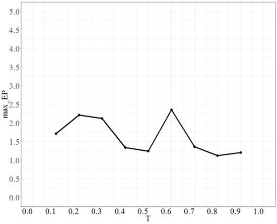
Figure 2. The behavior of max_EP as T changes.

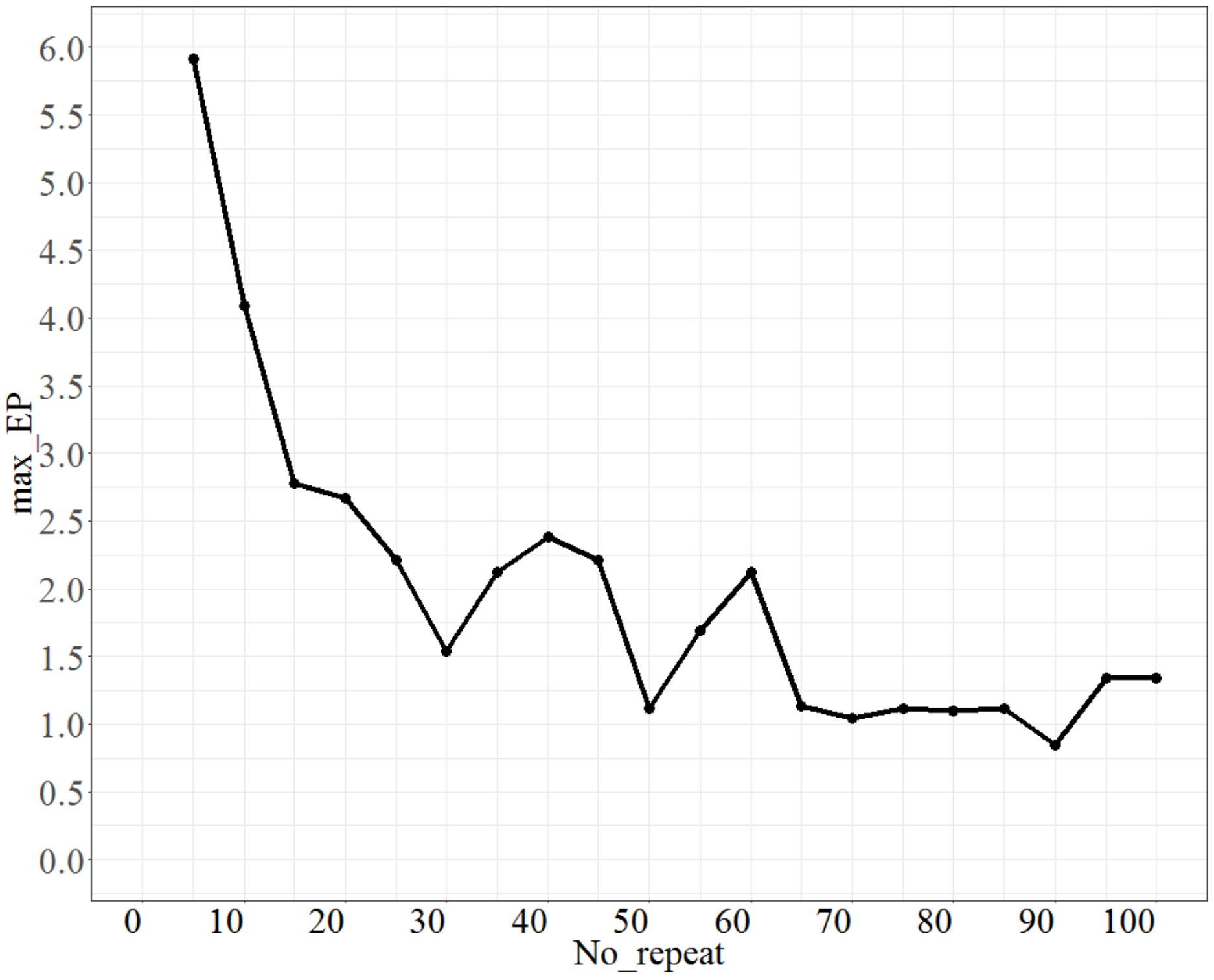
For testing No_repeat, No_d = 4, T = 0.8, Isize = 2, the test range of No_repeat was from 5 to 100, and each increment was 5 units. The max_EP is shown in Figure 3. As shown in Figure 3, as No_repeat increases, max_EP decreases significantly and approaches a stable state. However, the lowest maximum error percentage is at No_repeat = 90; thus, we set No_repeat to 90.

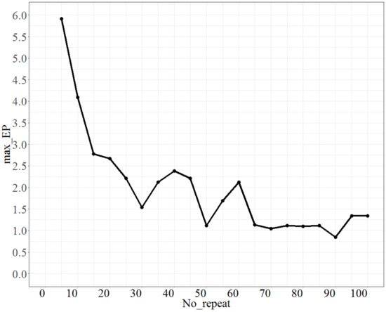
Figure 3. The behaviour of max_EPs as No_repeat changes.

Finally, the parameter Isize (the number of population groups) was calibrated; the parameter No_d was fixed at 4, T was fixed at 0.8, and No_repeat (the number of repetitions) was fixed at 90. The test range of Isize was from 2 to 10, and each increment was 1 unit. The max_EP is shown in Figure 4. As seen from Figure 4, the parameter Isize is relatively unstable, and the lowest value of max_EP is when Isize is 7; thus, Isize is chosen to be 7.

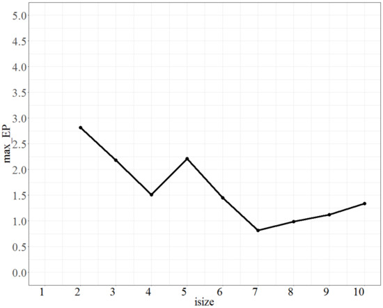
Figure 4. The max_EP plot as Isize varies.

Based on the tuning results, the parameters we selected for the small number of jobs were (4, 0.8, 90, 7) for (No_d, T, No_repeat, Isize).

4.2. Tuning Parameters for the Large-Size Problem

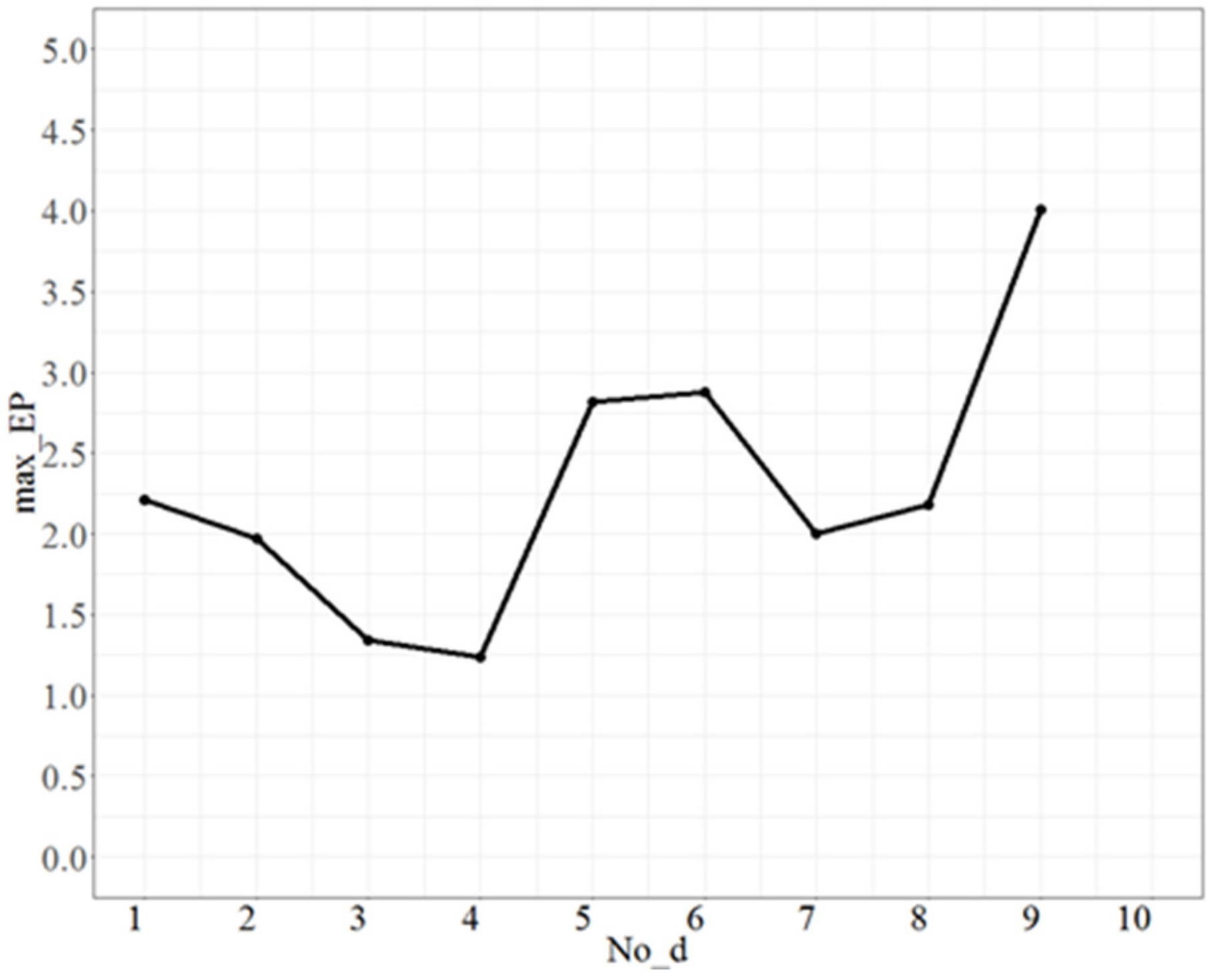
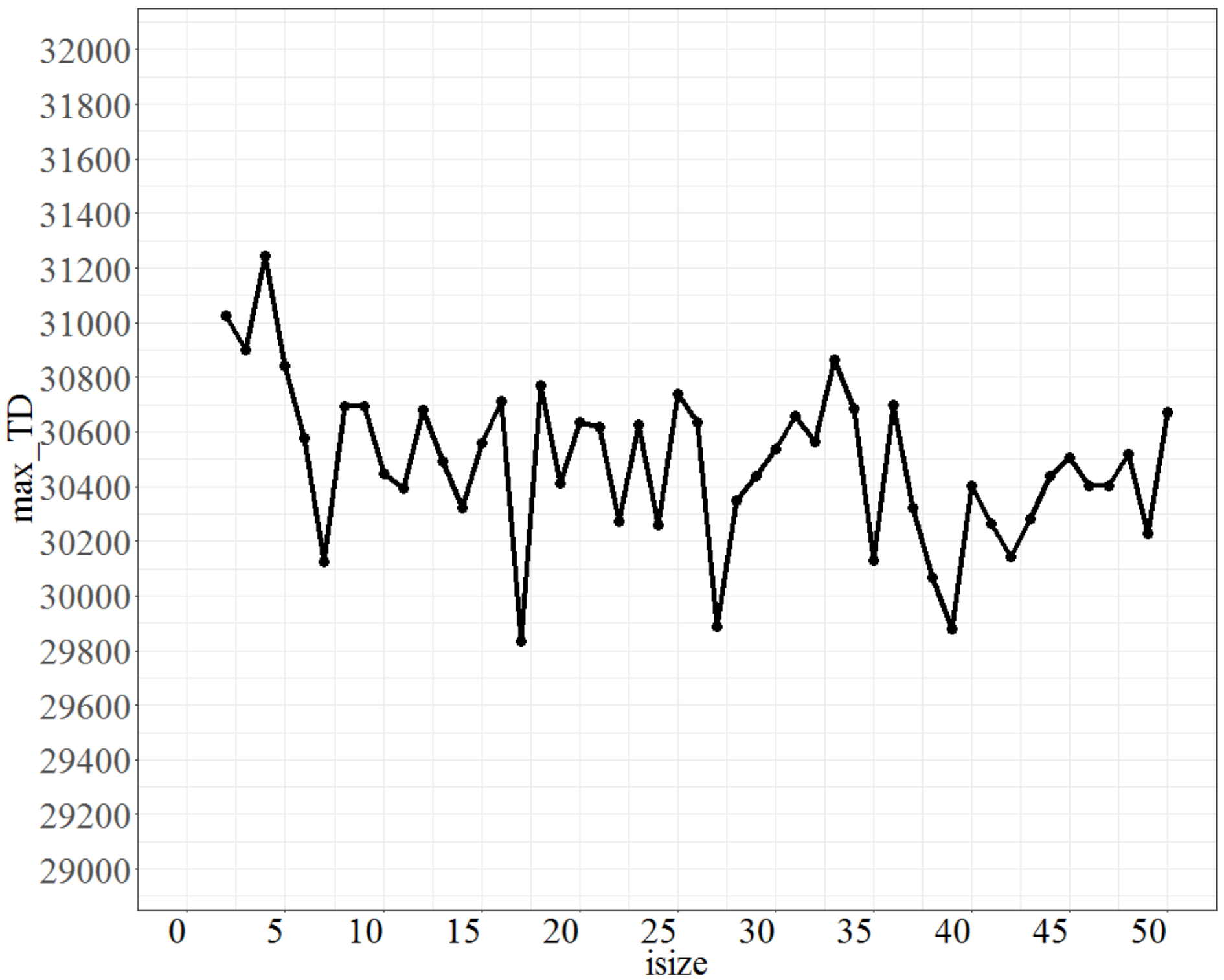
The parameters calibrated in the small-size problem were used as the basis of the tuning parameters for the large-size problem, i.e., No_repeat was 540 (= 90 * 6) times, T was 0.8, and Isize was 7. The test range of No_d was from 1 to 30, and each time, the increment was 1 unit. The maximum value (across 100 instances) of the objective function (total tardiness) is shown in Figure 5. Figure 5 shows that as No_d increases, the maximum value of the total tardiness, coded as max_TD, will increase. Because the errors are to be controlled within a predetermined 3%, the point No_d = 9, at which an approximately 3% increase in the max_TD is obtained from the lowest point (No_d at 5), was considered. Therefore, a No_d value of 9 is selected as the best fit.

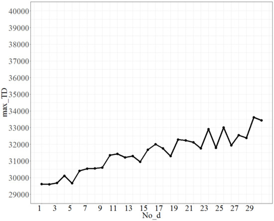
Figure 5. The plot of max_TD as No_d varies.

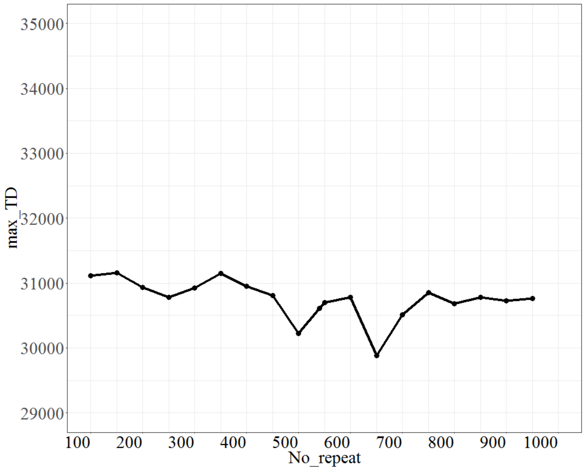
For testing No_repeat, the parameter No_d was fixed at 9, T at 0.8, and Isize at 7. The test range of No_repeat was from 100 to 950, and each increment was 50 units. The max_TD is shown in Figure 6. As shown in Figure 6, as No_repeat changes, max_TD reaches the lowest point for No_repeat at 500; thus, the best fit of No_repeat is 500.

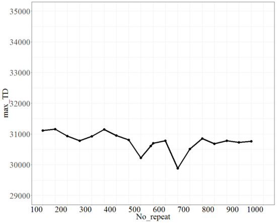
Figure 6. The plot of max_TD as No_repeat varies.

To test the parameter T (temperature), the parameter No_d was fixed at 9, No_repeat at 500, and Isize at 7. The value of T was increased by 0.1 units each time, ranging from 0.1 to 0.9. The max_TD is shown in Figure 7. Figure 7 shows that the max_TD increases as T increases from 0.3 to 0.5, and after 0.5 it drops rapidly to T = 0.8; thus, the parameter T is set to 0.8.

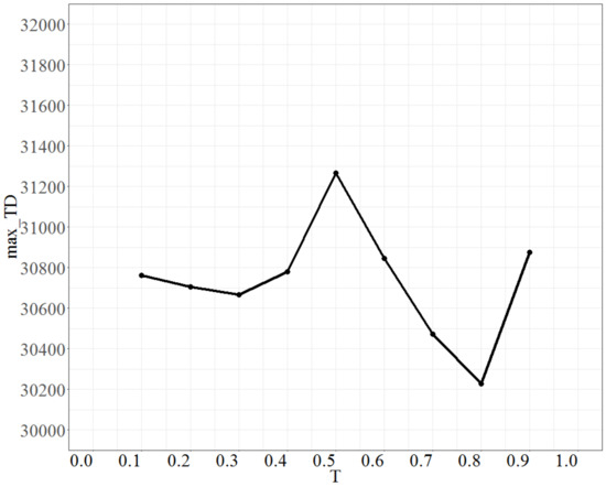
Figure 7. Plot of max_TD as T varies.

Finally, to tune the parameter Isize, the parameter No_d was fixed at 9, No_repeat at 500, and T at 0.8. The test range of Isize was from 1 to 50, and each increment was 1 unit. The max_TD values are shown in Figure 8. Figure 8 shows that Isize oscillates after 5, and that the oscillation range is set to be predetermined within 3% of the lowest maximum objective function, which is at Isize = 17; therefore, Isize at 7 is the best fit. Based on the tuning results, the preferred values of the parameters (No_d, No_repeat, T, Isize) are (9, 500, 0.8, 17) for a large number of jobs.

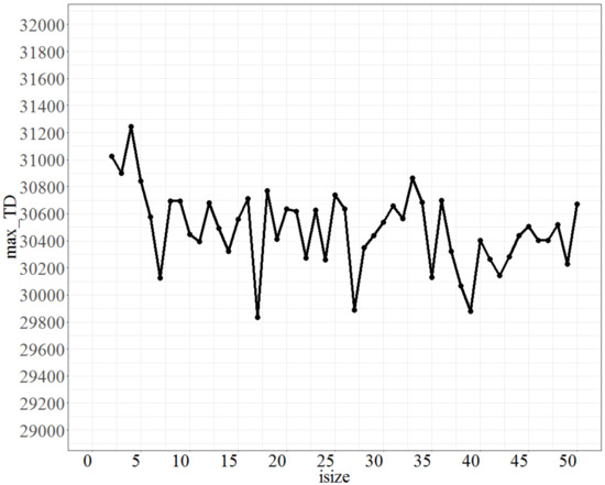
Figure 8. Plot of max_TD as Isize varies.

5. Computational Experiments and Analysis of Results

This section performs several problem instance tests to check the computational behaviors of the proposed heuristics and metaheuristics. The processing times, integers $t_j^{\left(1\right)}$ and $t_j^{\left(2\right)}$, were generated independently from two different uniform distributions (i.e., U [1, 100] and U [1, 200], respectively, see [16]), while the due dates, $d_j^{\left(v\right)}, \upsilon =1, 2$, are integers generated from a uniform distribution $TP{T}^{\left(\nu \right)}·U\left[1-\tau -\frac{\rho }{2}, 1-\tau +\frac{\rho }{2}\right]$, where $TP{T}^{\left(\nu \right)}={{\displaystyle \sum }}_{j=1}^n{t}_j^{\left(\nu \right)}$, $\rho and \tau$ represent the range of the due dates and the tardiness factor (see [28]), respectively. The values of $\tau$ were designed as 0.25 and 0.5, and the values of $\rho$ were 0.25, 0.5, and 0.75. For each combination of $\tau$ and $\rho$, 100 instances were generated as the test bank. In addition, as the number of explored nodes exceeds 10⁸, the branch-and-bound method is terminated and advances to the next set of instances. To determine the behavior of the B&B method, three local heuristics, and the PBIG algorithm, the experiments were examined for job sizes n = 8, 10, and 12 for the small-size problem and n = 60, 80, and 100 for the large-size problem. In total, 1800 problem instances were generated to solve the proposed problem. The four proposed algorithms were coded in FORTRAN 90. They were executed on a 16 GB RAM, 3.60 GHz, Intel(R) Core™ i7-4790 personal computer (64 bits) with Windows 7.

We then presented the results obtained from the designed simulation experiments to determine the efficiency of the proposed B&B method, three local heuristics, and the PBIG method. Figure 9 and Table 1, Table 2, Table 3, Table 4, Table 5 and Table 6 report the experimental results for the small-size case, while Figure 10 and Figure 11 and Table 4, Table 5, Table 6 and Table 7 summarize the experimental results for the large-size case.

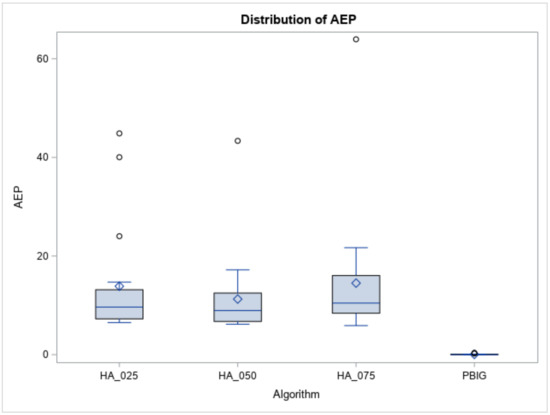
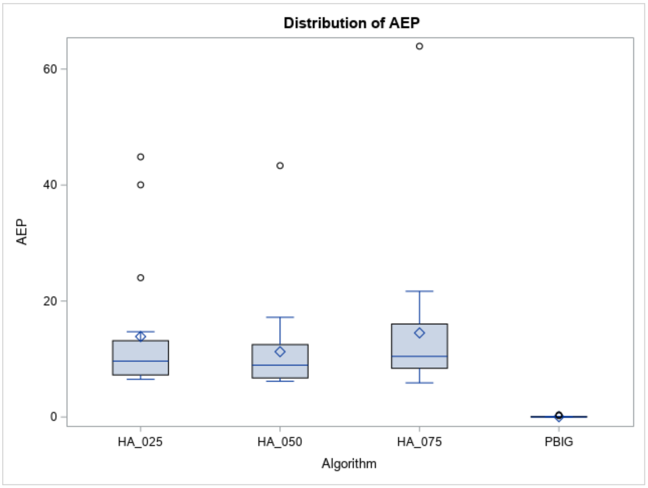
Figure 9. The distribution of the AEP.

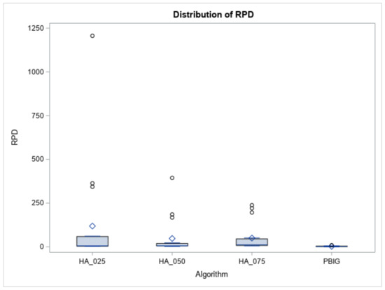
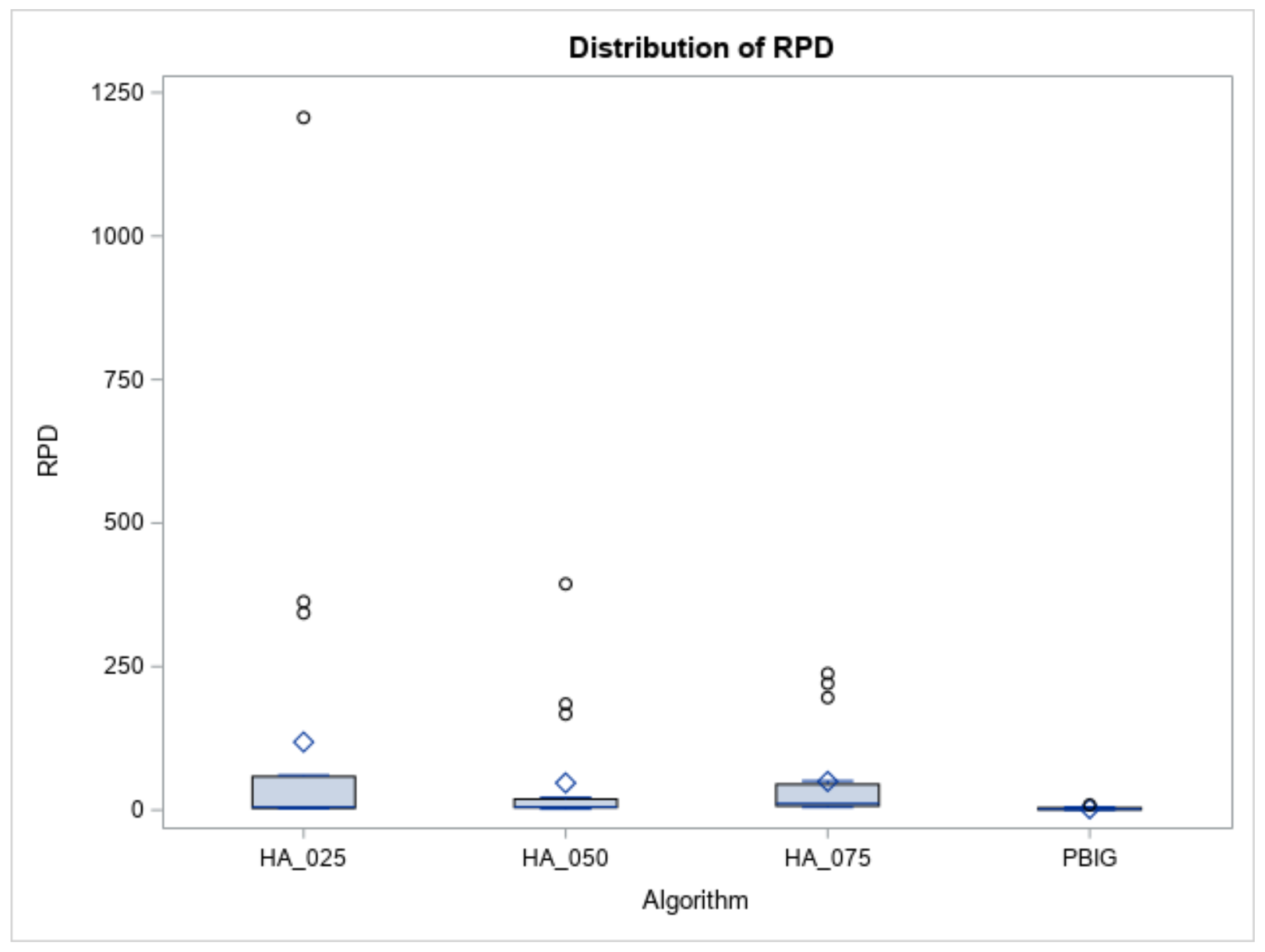
Figure 10. Boxplot of RPDs for heuristics and the PBIG algorithm.

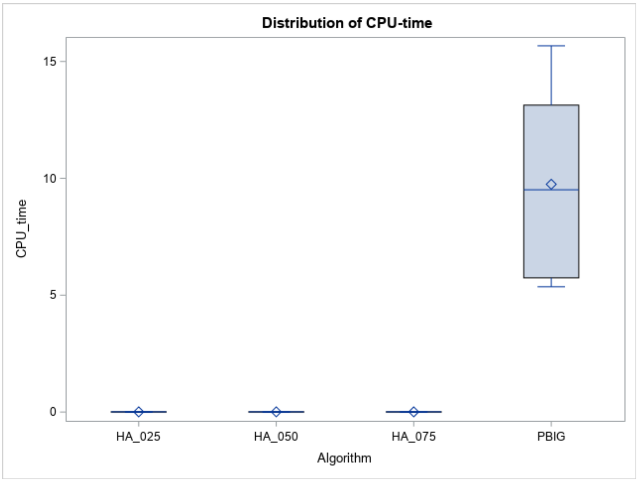
Figure 11. CPU times of heuristics and the algorithm for large n.

The $O_{i}s$ represent the optimal values received by running the B&B method, and the $H_{i}s$ record the solution obtained by each heuristic (or algorithm) for the test instances for the small-size case. To evaluate the performances of the three heuristics and the PBIG algorithm, the average error percentage (AEP =$100\left[mean\left(H\_i-O\_i\right)/O\_i\right]\%$) is used.

Table 1. The behavior of the B&B.

			Node		CPU_Time
n	$\mathit{\tau }$	$\mathit{\rho }$	Mean	Max	Mean	Max
8	0.25	0.25	1364.95	8041	0.00	0.03
		0.5	924.09	5872	0.00	0.03
		0.75	649.00	3344	0.00	0.02
	0.5	0.25	2169.63	12,975	0.01	0.03
		0.5	1441.85	11,199	0.00	0.03
		0.75	850.82	5707	0.00	0.02
10	0.25	0.25	18,383.94	155,332	0.08	0.58
		0.5	11,381.24	89,998	0.05	0.37
		0.75	6970.97	44,421	0.03	0.19
	0.5	0.25	47,294.00	634,898	0.18	2.25
		0.5	29,192.77	673,842	0.12	2.42
		0.75	25,154.69	717,700	0.10	2.59
12	0.25	0.25	319,906.05	4,022,178	1.91	22.11
		0.5	181,384.58	1,733,253	1.35	13.63
		0.75	77,810.74	603,931	0.63	4.62
	0.5	0.25	2,155,579.66	44,957,346	13.91	265.44
		0.5	517,837.47	19,204,302	3.74	125.30
		0.75	108,610.00	2,626,869	1.00	19.44
		mean	194,828.14	4,195,067	1.28	25.51

Table 1. The behavior of the B&B.

			Node		CPU_Time
n	$\mathit{\tau }$	$\mathit{\rho }$	Mean	Max	Mean	Max
8	0.25	0.25	1364.95	8041	0.00	0.03
		0.5	924.09	5872	0.00	0.03
		0.75	649.00	3344	0.00	0.02
	0.5	0.25	2169.63	12,975	0.01	0.03
		0.5	1441.85	11,199	0.00	0.03
		0.75	850.82	5707	0.00	0.02
10	0.25	0.25	18,383.94	155,332	0.08	0.58
		0.5	11,381.24	89,998	0.05	0.37
		0.75	6970.97	44,421	0.03	0.19
	0.5	0.25	47,294.00	634,898	0.18	2.25
		0.5	29,192.77	673,842	0.12	2.42
		0.75	25,154.69	717,700	0.10	2.59
12	0.25	0.25	319,906.05	4,022,178	1.91	22.11
		0.5	181,384.58	1,733,253	1.35	13.63
		0.75	77,810.74	603,931	0.63	4.62
	0.5	0.25	2,155,579.66	44,957,346	13.91	265.44
		0.5	517,837.47	19,204,302	3.74	125.30
		0.75	108,610.00	2,626,869	1.00	19.44
		mean	194,828.14	4,195,067	1.28	25.51

Table 1 presents the capability of the B&B method. All tested problem instances could be solved before 10⁸ nodes. The computation CPU times, including the average execution times and maximum execution times (in seconds), increased dramatically as n increased (Columns 6 and 7, Table 1). As n increased, the mean and maximum nodes also increased (Columns 4 and 5, Table 1). Table 2 reports the results of CPU times and node numbers for the small-size n, $\tau$, and $\rho$.

Table 2. Summary of the results of the B&B method.

		Node		CPU_Time
		Mean	Max	Mean	Max
n	8	1233.390	7856.333	0.002	0.027
	10	23,062.935	386,031.833	0.093	1.400
	12	560,188.083	12,191,313.167	3.757	75.090
$\tau$	0.25	68,752.840	740,707.778	0.450	4.620
	0.5	320,903.432	7,649,426.444	2.118	46.391
$\rho$	0.25	424,116.372	8,298,461.667	2.682	48.407
	0.5	123,693.667	3,619,744.333	0.877	23.630
	0.75	36,674.370	666,995.333	0.293	4.480

Table 2. Summary of the results of the B&B method.

		Node		CPU_Time
		Mean	Max	Mean	Max
n	8	1233.390	7856.333	0.002	0.027
	10	23,062.935	386,031.833	0.093	1.400
	12	560,188.083	12,191,313.167	3.757	75.090
$\tau$	0.25	68,752.840	740,707.778	0.450	4.620
	0.5	320,903.432	7,649,426.444	2.118	46.391
$\rho$	0.25	424,116.372	8,298,461.667	2.682	48.407
	0.5	123,693.667	3,619,744.333	0.877	23.630
	0.75	36,674.370	666,995.333	0.293	4.480

Regarding the behaviors of the three heuristics and the PBIG, their AEPs are displayed in Table 3. All AEPs of the three heuristics and the PBIG algorithm increased slightly as n increased. Overall, the PBIG algorithm, with a mean AEP of less than 0.14% for n = 8, 10, and 12, performed the best. Figure 9 indicates the AEPs (output results) of the three heuristics and the PBIG algorithm. Since the computer execution times are all less than 0.1 s, they are not reported here.

Table 3. The AEPs of the heuristics and the PBIG algorithm.

		HA_025	HA_050	HA_075	PBIG
n	8	10.301	8.121	9.948	0.004
	10	14.283	9.408	12.235	0.027
	12	17.045	16.276	21.333	0.130
$\tau$	0.25	18.925	13.966	19.432	0.011
	0.5	8.827	8.570	9.578	0.096
$\rho$	0.25	7.850	7.623	7.642	0.020
	0.5	10.806	8.890	12.193	0.046
	0.75	22.972	17.291	23.681	0.094

Table 3. The AEPs of the heuristics and the PBIG algorithm.

		HA_025	HA_050	HA_075	PBIG
n	8	10.301	8.121	9.948	0.004
	10	14.283	9.408	12.235	0.027
	12	17.045	16.276	21.333	0.130
$\tau$	0.25	18.925	13.966	19.432	0.011
	0.5	8.827	8.570	9.578	0.096
$\rho$	0.25	7.850	7.623	7.642	0.020
	0.5	10.806	8.890	12.193	0.046
	0.75	22.972	17.291	23.681	0.094

For the behaviors of the proposed four algorithms, we performed an analysis of variance (ANOVA) on the AEPs. As shown in Table 4 (Columns 2 and 3), the Kolmogorov–Smirnov test was significant, with a p value $<$0.01. This implies that the samples of AEPs do not follow the normal distribution. Therefore, based on the ranks of AEPs, the Kruskal–Wallis test was utilized to determine if the populations of AEPs came from the same population or not. Column 2 of Table 5 confirmed that the proposed three heuristics and the PBIG algorithm were indeed significantly different, with a p value < 0.001.

Table 4. Normality Tests for small n and large n.

	Small n		Large n
Method of Normality Test	Statistic	p Value	Statistic	p Value
Shapiro–Wilk normality test	0.7957	<0.0001	0.6225	<0.0001
Kolmogorov–Smirnov test	0.1753	<0.0100	0.1805	<0.0100
Cramer–von Mises normality test	0.5897	<0.0050	0.6418	<0.0050
Anderson–Darling normality test	3.5444	<0.0050	4.2936	<0.0050

Table 4. Normality Tests for small n and large n.

	Small n		Large n
Method of Normality Test	Statistic	p Value	Statistic	p Value
Shapiro–Wilk normality test	0.7957	<0.0001	0.6225	<0.0001
Kolmogorov–Smirnov test	0.1753	<0.0100	0.1805	<0.0100
Cramer–von Mises normality test	0.5897	<0.0050	0.6418	<0.0050
Anderson–Darling normality test	3.5444	<0.0050	4.2936	<0.0050

Table 5. Kruskal–Wallis Test.

Kruskal–Wallis Test
	Small n	Large n
Chi-square	40.8017	29.6735
DF	3	3
Pr > Chi-square	<0.0001	<0.0001

Table 5. Kruskal–Wallis Test.

Kruskal–Wallis Test
	Small n	Large n
Chi-square	40.8017	29.6735
DF	3	3
Pr > Chi-square	<0.0001	<0.0001

In addition, heuristics HA_025, HA_050, HA_075, and the PBIG were further used to conduct pairwise differences. The Dwass–Steel–Critchlow–Fligner (DSCF) procedure was applied (see [29]). Table 6 confirms that the mean ranks of AEPs were grouped into two subsets under the level of significance of 0.05. From Columns 3 and 4 of Table 6, the PBIG (with the AEP of 0.005) was placed in a better behavior group, while HA_025 (with the AEP of 0.014), HA_050 (with the AEP of 0.011), and HA_075 (with the AEP of 0.015) were placed in a worse performance set.

Table 6. DSCF pairwise comparison.

Pairwise Comparison	DSCF
	Small n		Large n
Between Algorithms	Statistic	p Value	Statistic	p Value
HA_025 vs. HA_050	1.2976	0.7955	0.1790	0.9993
HA_025 vs. HA_075	0.4922	0.9855	2.3714	0.3359
HA_025 vs. PBIG	7.2880	<0.0001	5.2350	0.0012
HA_050 vs. HA_075	1.5213	0.7044	3.0426	0.1371
HA_050 vs. PBIG	7.2880	<0.0001	5.5035	0.0006
HA_075 vs. PBIG	7.2880	<0.0001	6.7563	<0.0001

Table 6. DSCF pairwise comparison.

Pairwise Comparison	DSCF
	Small n		Large n
Between Algorithms	Statistic	p Value	Statistic	p Value
HA_025 vs. HA_050	1.2976	0.7955	0.1790	0.9993
HA_025 vs. HA_075	0.4922	0.9855	2.3714	0.3359
HA_025 vs. PBIG	7.2880	<0.0001	5.2350	0.0012
HA_050 vs. HA_075	1.5213	0.7044	3.0426	0.1371
HA_050 vs. PBIG	7.2880	<0.0001	5.5035	0.0006
HA_075 vs. PBIG	7.2880	<0.0001	6.7563	<0.0001

Regarding the test performance on the large-sized jobs, we tested the number of jobs at n = 60, 80, and 100. For each combination of $\tau , \rho$, and n, we generated one hundred problem instances to evaluate the performances of the proposed methods. Overall, we examined and tested 1800 random problem instances. The measurement is the relative percent deviation (RPD), where RPD is defined as $100\left[mean\left(H_i-Bes{t}_i\right)/Bes{t}_i\right]\%$). It was noted that $H_i$ was the value of the objective function found in each algorithm, and $Bes{t}_i$ was the smallest objective function between the four methods. All of the average RPDs of the four algorithms are recorded in Table 7. As shown in Table 7, PBIG provided the lowest value of RPDs, no matter the value of n. Figure 10 displays the boxplots of the RPDs for the three heuristics and the PBIG algorithm.

Furthermore, using ANOVA to determine whether the RPDs follow a normal distribution or not, Table 4 (Columns 4 and 5) indicates that the normality assumption is not met, since the p value < 0.01. Therefore, Column 3 of Table 5 indicates that a Kruskal–Wallis test, which is based on ranks of RPDs, clearly states that “the RPD samples belong to different distributions” when the p value < 0.001. Thus, the DSCF procedure was adopted to compare the pairwise differences between the four methods. Columns 4 and 5 of Table 6 report that the PBIG algorithm was placed in a better set; meanwhile, the other three heuristics belong to another set for a large number of job cases. Furthermore, the boxplots in Figure 10 show that the RPDs of the PBIG had a smaller range than those of the three heuristics. This implies that the PBIG could find a stable and accurate solution when compared to the other three heuristic methods in the large-size problem cases. For the computational time or CPU times (in seconds), Figure 11 displays the boxplots of the times for the heuristics and PBIG algorithm. Three heuristics take less than one second, while PBIG takes less than 15 s.

Table 7. The RPD values of the four algorithms.

		HA_025	HA_050	HA_075	PBIG
n	60	214.519	72.929	47.249	2.521
	80	69.519	33.830	50.049	1.773
	100	71.282	35.274	52.304	2.665
τ	0.25	232.728	90.140	90.587	3.387
	0.5	4.152	4.549	9.148	1.253
ρ	0.25	4.678	4.578	6.358	1.855
	0.5	30.137	11.730	27.567	2.163
	0.75	320.506	125.724	115.677	2.941

Table 7. The RPD values of the four algorithms.

		HA_025	HA_050	HA_075	PBIG
n	60	214.519	72.929	47.249	2.521
	80	69.519	33.830	50.049	1.773
	100	71.282	35.274	52.304	2.665
τ	0.25	232.728	90.140	90.587	3.387
	0.5	4.152	4.549	9.148	1.253
ρ	0.25	4.678	4.578	6.358	1.855
	0.5	30.137	11.730	27.567	2.163
	0.75	320.506	125.724	115.677	2.941

6. Conclusions

In this article, we introduced scenario-dependent due dates and scenario-dependent processing times into a single-machine environment. We built one lower bound and eight dominances in the B&B method for finding a robust optimal schedule for a small number of jobs (up to n = 12). The reason for this was that the proposed properties and lower bound in the B&B method were not strong. Three different values for a parameter in one local search heuristic were proposed. Furthermore, a PBIG algorithm was provided to tackle this problem for large-sized job cases. We also used statistical methods to evaluate and examine the performances of all proposed algorithms. Undoubtedly, to search the robust job sequences, the PBIG algorithm performs the best not only in optimality but also in reliability (less dispersion), although the PBIG requires more CPU time.

Possible future studies include (1) the study of other scheduling problem characteristics such as job ready times, which may also incur uncertain features. (2) One future study may consider a scenario-dependent single-machine model with multiple objective functions. (3) This paper only addressed two scenarios, and we may extend it to more than two scenarios. One shortcoming of PBIG is that we use $\max \_\mathrm{EP}$ or max_TD to find the values of parameters, instead of AEP. Therefore, one more future study may consider other population-based genetic algorithms for this model.

References

- Shi, Y.; Boudouh, T.; Grunder, O. A robust optimization for a home health care routing and scheduling problem with consideration of uncertain travel and services times. Transp. Res. Part E 2019, 128, 52–95. [Google Scholar] [CrossRef]
- Assavapokee, T.; Realff, M.J.; Ammons, J.C.; Hong, I.-H. Scenario relaxation algorithm for finite scenario-based min–max regret and min–max relative regret robust optimization. Comput. Oper. Res. 2008, 35, 2093–2102. [Google Scholar] [CrossRef]
- Hazır, O.; Haouari, M.; Erel, E. Robust scheduling and robustness measures for the discrete time/cost trade-off problem. Eur. J. Oper. Res. 2010, 207, 633–643. [Google Scholar] [CrossRef]
- Ouaret, S.; Kenné, J.P.; Gharbi, A. Stochastic optimal control of random quality deteriorating hybrid manufacturing/remanufacturing systems. J. Manuf. Syst. 2018, 49, 172–185. [Google Scholar] [CrossRef]
- Daniels, R.L.; Kouvelis, P. Robust scheduling to hedge against processing time uncertainty in single-stage production. Manag. Sci. 1995, 41, 363–376. [Google Scholar] [CrossRef]
- Yang, J.; Yu, G. On the robust single machine scheduling problem. J. Comb. Optim. 2002, 6, 17–33. [Google Scholar] [CrossRef]
- Kouvelis, P.; Yu, G. Robust Discrete Optimization and Its Applications; Kluwer Acaemic Publishers: Alphen aan den Rijn, The Netherlands, 1997. [Google Scholar]
- Aytug, H.; Lawley, M.; McKay, K.; Mohan, S.; Uzsoy, R. Executing production scheduling in the face of uncertainties: A review and some future directions. Eur. J. Oper. Res. 2005, 161, 86–110. [Google Scholar] [CrossRef]
- Mastrolilli, M.; Mustsanas, N.; Svensson, O. Single machine scheduling with scenarios. Theor. Comput. Sci. 2013, 477, 57–66. [Google Scholar] [CrossRef]
- Niu, S.; Song, S.; Ding, J.Y.; Zhang, Y.; Chiong, R. Distributionally robust single machine scheduling with the total tardiness criterion. Comput. Oper. Res. 2019, 101, 13–28. [Google Scholar] [CrossRef]
- Yue, F.; Song, S.; Jia, P.; Wu, G.; Zhao, H. Robust single machine scheduling problem with uncertain job due dates for industrial mass production. J. Syst. Eng. Electron. 2020, 31, 350–358. [Google Scholar] [CrossRef]
- Framinan, J.M.; Perez-Gonzalez, P. Order scheduling with tardiness objective: Improved approximate solutions. Eur. J. Oper. Res. 2018, 266, 840–850. [Google Scholar] [CrossRef] [Green Version]
- Ta, Q.C.; Billunt, J.-C.; Bouquard, J.-L. Matheuristic algorithms for minimizing total tardiness in the m-machine flow-shop scheduling problem. J. Intell. Manuf. 2018, 29, 617–628. [Google Scholar] [CrossRef]
- Koulamas, C. The single-machine total tardiness scheduling problem: Review and extensions. Eur. J. Oper. Res. 2010, 202, 1–7. [Google Scholar] [CrossRef]
- Sen, T.; Sulek, J.M.; Dileepan, P. Static scheduling research to minimize weighted and unweighted tardiness: A state-of-the-art survey. Int. J. Prod. Econ. 2003, 83, 1–12. [Google Scholar] [CrossRef]
- Wu, C.C.; Bai, D.; Zhang, X.; Cheng, S.R.; Lin, J.C.; Wu, Z.L.; Lin, W.C. A robust customer order scheduling problem along with scenario-dependent component processing times and due dates. J. Manuf. Syst. 2021, 58, 291–305. [Google Scholar] [CrossRef]
- Pinedo, M.L. Scheduling: Theory, Algorithms, and Systems, 3rd ed.; Prentice Hall: Hoboken, NJ, USA, 2008. [Google Scholar]
- Aloulou, M.A.; Della Croce, F. Complexity of single machine scheduling problems under scenario-based uncertainty. Oper. Res. Lett. 2008, 36, 338–342. [Google Scholar] [CrossRef] [Green Version]
- Kasperski, A.; Zielinski, P. Minmax (regret) scheduling problems. In Sequencing and Scheduling with Inaccurate Data; Sotskov, Y.N., Werner, F., Eds.; Nova Science Publishers, Inc.: Hauppauge, NY, USA, 2014. [Google Scholar]
- Liu, F.; Wang, S.; Hong, Y.; Yue, X. On the Robust and Stable Flowshop Scheduling under Stochastic and Dynamic Disruptions. IEEE Trans. Eng. Manag. 2017, 64, 539–553. [Google Scholar] [CrossRef]
- Wang, D.J.; Qiu, H.; Wu, C.C.; Lin, W.C.; Lai, K.; Cheng, S.R. Dominance rule and opposition based particle swarm optimization for two-stage assembly scheduling with time cumulated learning effect. Soft Comput. 2019, 23, 9617–9628. [Google Scholar] [CrossRef]
- Wang, J.B.; Gao, M.; Wang, J.J.; Liu, L.; He, H. Scheduling with a position-weighted learning effect and job release dates. Eng. Optim. 2020, 52, 1475–1493. [Google Scholar] [CrossRef]
- Porta, J.; Parapar, J.; Doallo, R.; Barbosa, V.; Santé, I.; Crecente, R.; Díaz, C. A population-based iterated greedy algorithm for the delimitation and zoning of rural settlements. Comput. Environ. Urban Syst. 2013, 39, 12–26. [Google Scholar] [CrossRef]
- Ruiz, R.; Stützle, T. A simple and effective iterated greedy algorithm for the permutation flowshop scheduling problem. Eur. J. Oper. Res. 2007, 177, 2033–2049. [Google Scholar] [CrossRef]
- Dubois-Lacoste, J.; Pagnozzi, F.; Stützle, T. An iterated greedy algorithm with optimization of partial solutions for the makespan permutation flowshop problem. Comput. Oper. Res. 2017, 81, 160–166. [Google Scholar] [CrossRef]
- Msakni, M.K.; Khallouli, W.; Al-Salem, M.; Ladhari, T. Minimizing the total completion time in a two-machine flowshop problem with time delays. Eng. Optim. 2016, 48, 1164–1181. [Google Scholar] [CrossRef]
- Bouamama, S.; Blum, C.; Boukerram, A. A population-based iterated greedy algorithm for the minimum weight vertex cover problem. Appl. Soft Comput. 2012, 12, 1632–1639. [Google Scholar] [CrossRef]
- Fisher, M.L. A dual algorithm for the one-machine scheduling problem. Math. Program. 1976, 11, 229–251. [Google Scholar] [CrossRef]
- Hollander, M.D.; Wolfe, A.; Chicken, E. Nonparametric Statistical Methods, 3rd ed.; John Wiley & Sons, Inc.: Hoboken, NJ, USA, 2014. [Google Scholar]
Publisher’s Note: MDPI stays neutral with regard to jurisdictional claims in published maps and institutional affiliations. |
© 2022 by the authors. Licensee MDPI, Basel, Switzerland. This article is an open access article distributed under the terms and conditions of the Creative Commons Attribution (CC BY) license (https://creativecommons.org/licenses/by/4.0/).