Abstract
A moving spatial turbulence model is developed for rotorcraft maneuvering simulation under different flight conditions. The recursive algorithms are adopted to model its distributed longitudinal turbulence components, which are correlated with the lateral and vertical axes to form a local spatial turbulence field. The flow field is constrained around the rotorcraft by following its movement, and the corresponding turbulence components are updated at a constant spatial interval. The statistical properties along the longitudinal, lateral, and vertical directions have been validated against the von Kármán theory. A synthetic simulation environment consisting of a flight dynamics model and a pilot model is constructed to demonstrate the effectiveness of the turbulence model. Its performance is validated by comparing the power spectral densities of both rotorcraft responses and pilot controls in turbulence against flight test data. The piloted simulation results on an Approach-to-Hovering task show that the handling qualities ratings are susceptive to the level of turbulence and significantly increase when performing aggressive controls. The simulation also accurately predicts the expected effect of varied aircraft speed, wind speed, turbulence intensity, and stability augmentation system on piloted handling qualities rating for rotorcraft flight in turbulence.
MSC:
62-08
1. Introduction
Rotorcraft often encounter atmospheric turbulence when operating near the ground. The undulating turbulence properties and wind speed with altitude can lead to a variation of rotorcraft dynamics characteristics [1], posing a safety issue for rotorcraft operation under some circumstances due to the requirement of extra pilot efforts for rejection of turbulence and dealing with adverse motion characteristics of the vehicle. A turbulence model with a good level of accuracy is vital to study and reduce the potential adverse effects on rotorcraft operation by providing a high-fidelity simulation.
Three mainstream turbulence models have been developed for prediction of rotorcraft response to turbulence. The earliest developments were to produce spatially distributed turbulence components directly based on spectral functions. Campbell and Sanborn [2] proposed a Monte Carlo method to generate three-dimensional frozen turbulence. Three-dimensional Gaussian white noise signals were generated in the spatial-frequency domain, multiplied by transfer functions with desired spectra, and then were transformed back to form spatially distributed turbulence components. Robinson et al. [3] developed a full-field atmospheric turbulence model for use with piloted rotorcraft simulation. Spatial turbulence samples were generated using a summation of sinusoids to match the von Kármán spectra. Dang et al. [4] came up with a parallel method running on a number of processors to speed up the summation-of-sinusoids algorithms for turbulence simulation and rotorcraft-response prediction. The spatial turbulence models are capable of adapting to turbulence proprieties varied with altitude and vehicle speed. However, these models require heavy computations to achieve improved simulation accuracy and large storage for large or full-field turbulence. McFarland and Duisenberg [5] turned to produce a time-domain turbulence field by spectral functions in temporal frequency. Turbulence velocity components were generated in front of the main rotor with the assumed “frozen field” and floated downstream when the rotorcraft flew forward to form a two-dimensional flow field. The turbulence components at any point were obtained by the Gaussian interpolation in the lateral direction. Ji et al. [6] extended this work by developing high-order filters with the approximate von Kármán spectra [7] and establishing mathematically rigorous spatial correlation along the lateral and vertical axes [8] to form a three-dimensional turbulence field. Different from the physics-based approach, the Control Equivalent Turbulence Input (CETI) models [9,10,11] produced the time histories of control inputs to rotorcraft with specific Power Spectral Densities (PSD) to simulate the same effect of turbulence. The spectral functions were identified from flight test data in turbulent wind conditions. They were originally developed for control system optimization, in-flight simulation, and pilot training in hover/low-speed flight, and were later extended to forward flight [10] and multi-input/multi-output applications [11]. The temporal turbulence models generate a local turbulence field around a rotorcraft or the time histories of CETI and thus significantly reduce requirements of computation and storage. However, they cannot adapt to various flight speeds due to the fact that the spectral functions of turbulence components or control inputs are in temporal-frequency form and should be implemented under a steady airspeed for the time histories of turbulence components or CETI signals. Progress in Computational Fluid Dynamics (CFD) techniques offered another way to model a turbulence field over complex terrain [12]. Henriquez Huecas et al. [13] put forward a synthetic eddy method for use in flight simulation and handling qualities analysis. Eddies were generated with a random distribution within a control volume around a rotorcraft and were converted to form a time-varying turbulence field. Liu et al. [14] used a well-established large-eddy simulation model to generate highly resolved wind fields over a mountainous region. The application of the CFD methods in natural turbulence modeling for aircraft flight analysis is constrained by extensive computations required to generate a flow field.
This paper presents a moving spatial turbulence model with low requirements of computation and storage for efficient implementation and the capability of adapting to various flight conditions during maneuvering. The paper is structured as below. Section 2 will give the development and initial validation of the turbulence model. In Section 3, the turbulence model will be integrated into a simulation environment with a rotorcraft dynamics model and a pilot model. The validation of the simulation model will be given there. Rotorcraft maneuvering flight in turbulent wind with different flight speeds and altitudes will be investigated in Section 4. Finally, the results are discussed in Section 5, and the conclusions are drawn in Section 6.
2. Moving Spatial Turbulence Model
2.1. Recursive Algorithms for Spatial Turbulence Components
Turbulence components will be produced by passing spatially distributed white noise samples through recursive algorithms. The von Kármán spectra satisfy the Kolmogorov −5/3 decay law and correlate well with experimental data [15], and therefore are chosen to derive the recursive algorithms. The most challenging problem for the application of the von Kármán spectra arises from their irrational forms. However, high-order rational approximants to the spectra were easily obtained by the least-squares approximation method [7],
where are the approximate spectra for longitudinal, lateral, and vertical turbulence components, is the spatial frequency, are the standard deviations of the turbulence components, are the integral length scales, and is the circumference ratio. The coefficients are as follows,
Writing gives the frequency response functions
where and are the frequency response functions for longitudinal, lateral, and vertical turbulence components in spatial frequency.
The bilinear transform [16] will be used to convert Equation (2) to fucntions. Substituting into the longitudinal frequency response function, we get that
where and are
and the coefficients and are
In view that
where represents longitudinal turbulence component sample with unit variance, and represents white noise sample along the longitudinal direction with unit spectrum. Thus, the spectrum of the white noise sample is
However, the unit-variance white noise sample is more widely used in simulation practice, and the variance is
where is the spectrum of the white noise sample , and is the Nyquist frequency in the spatial domain.
Combining Equations (8) and (9) arrives at
As a consequence, the relationship between and is
The transform from the white noise sample to the longitudinal turbulence component sample is
Finally, substituting Equation (3) into Equation (12), after cross multiplying and simplifying, the difference equation for the longitudinal turbulence component sample is
where and are the longitudinal turbulence sample and spatially distributed white noise sample at the location , and
The difference equation for lateral turbulence component sample was obtained by conducting the same procedures for the lateral frequency response function in Equation (2). The recursive algorithm is
where is the lateral turbulence component sample with unit variance, and the coefficients , , and are
The difference equation for the vertical turbulence component sample is similar to that for the lateral case in Equation (15). Thus, Equations (13) and (15) give the recursive algorithms for spatially distributed turbulence components with unit variance. For a rotorcraft encountering a patch of turbulence at low altitude, the integral length scales are assumed constant and are determined by the intermediate height of the turbulence field and the underlying terrain roughness [1]
The turbulence intensities will vary with the altitude and the underlying terrain roughness as well as be influenced by the local wind speed
The wind speed varies with the altitude and is formulated by the power law [1],
where is the wind speed at the altitude of 10 m. The exponent is an empirically derived coefficient dependent upon the underlying terrain roughness,
The turbulence intensities , and are easily obtained with Equations (20) and (21) for a rotorcraft flying with varied flight altitude, and thus turbulence components along the longitudinal direction of airspeed are
2.2. Moving Spatial Turbulence Field
The turbulence components produced by the recursive algorithms in Equations (13) and (15) are correlated to form correlated spatial turbulence filters for their expansion in lateral and vertical axes. It was proven that the linear transformation with the Cholesky factor is optimal to relate dependent turbulence components with desired correlations [8]. For sets of dependent turbulence component samples along the longitudinal direction, the covariance matrices , and can be obtained by the spatial correlation of the von Kármán theory [15]
where , , , . and are the lateral and vertical coordinates of the and sets of dependent turbulence component samples, is the gamma function, and is the modified Bessel function of the second kind.
The lower triangular factors can be solved by the Cholesky factorization to the covariance matrices [16] as follows
Finally, dependent turbulence component samples are obtained through the transformation
with
where are the dependent turbulence components of the samples at the position , and are the independent turbulence components. Thus, combing the recursive algorithms in Equations (13) and (15) and the transformation in Equation (26), sets of correlated spatial filters can be formed with sets of independent white noise samples.
With the correlated spatial filters, a turbulence field of the cuboid ABCDEFGH is formed around a flying rotorcraft, as shown in Figure 1a. The length of the turbulence field is , the width is , and the height is . The turbulence field will move forward along the longitudinal direction of airspeed to keep around the vehicle, and it can also rotate along the lateral and vertical axes to keep the front surface ABCD perpendicular to the airspeed . The turbulence field is divided into nodes with the intervals and along the longitudinal, lateral, and vertical axes, as shown in Figure 1b. The sets of correlated spatial filters are placed on the grid nodes of the surface ABCD. The filters will update once the turbulence field moves forward one step and the new turbulence components are fixed at the inertial space where they are produced. Thus, every node of the grid will be filled with turbulence components by the forward movement of the turbulence field.
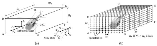
Figure 1.
Moving spatial turbulence field. (a) Geometry; (b) Grid.
The airspeed is the difference between the ground speed and the wind speed , as shown in Figure 2. The components and of the wind speed are obtained by transforming the wind speed magnitude into the North-East-Down (NED) axes with the wind direction
.
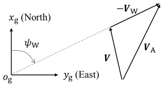
Figure 2.
Relationship among wind speed , ground speed , and airspeed .
A turbulence coordinate system is established at the center of the surface ABCD. The -axis points at the opposite direction of the airspeed, the -axis points to the right direction of the aircraft, and the -axis points up. The turbulence field is softly constrained to the movement of the aircraft at the Center of Gravity (CG) with
where and are the coordinates of the CG, is the radius of the main rotor. The initial condition of the CG of aircraft is
where represents time. At each simulation step, as the aircraft moves meters forward with respect to the air, the turbulence field has to move up steps with the step size to satisfy the constraint in Equation (28)
where ⌈ ⌉ is the ceiling operator. Since is not often equal to , the coordinate of the aircraft CG varies with the rotorcraft speed
where is the simulation number and is the simulation step. To keep the front surface ABCD perpendicular to the airspeed , the heading and climb angles of airspeed are defined
where and are the heading and climb angles of airspeed, and , and are the airspeed components in the NED system. Thus, the transformation matrix from the NED axes to the turbulence axes is
where and are the direction cosine matrices rotating round lateral and vertical axes, respectively.
With the kinetics of the turbulence field, the coordinates of each rotorcraft aerodynamic element, taking the fuselage for example, in the turbulence axes can be calculated by
where and are the coordinates of the fuselage and CG in the body axes, as well as and are the coordinates of the fuselage and CG in the turbulence axes.
With the coordinates , the turbulence components of the fuselage are obtained by the nearest interpolation to the turbulence field and denoted as . After transforming into the NED axes, the turbulence components of the fuselage for the flight dynamics model are,
where is the transformation matrix from the turbulence axes to the NED axes, and are the turbulence components of the fuselage in the NED axes.
With coordinates derived from the flight dynamics model and then repeating the above procedures, turbulence components of each aerodynamic element of the rotorcraft can be calculated and then transferred to the flight dynamics model for simulation.
2.3. Initial Validation of Turbulence Model
The statistical property of the moving spatial turbulence model is validated against the theoretical von Kármán model before taking a further insight into its effect on rotorcraft operations. The turbulence model is integrated with a hovering UH-60 rotorcraft flying toward freestream turbulence. The length of the rotorcraft is 19.76 m including the main rotor, the height is 5.13 m, and the main rotor diameter is 16.36 m. Therefore, the turbulence field is set with m, m, and m. The grid intervals are set with m, and the grid nodes are . The wind condition is set with m/s, m, and m to simulate turbulence over a suburban area [17].
Figure 3 shows a slice of turbulence components over the horizontal plane. It is observed that all three turbulence components vary randomly along the longitudinal and lateral axes, in which longitudinal and lateral components show more regularity over the flow field than the vertical components. This reflects the fact that the longitudinal and lateral integral length scales are larger than the vertical one, resulting in the corresponding turbulence components being more highly correlated over the flow field.
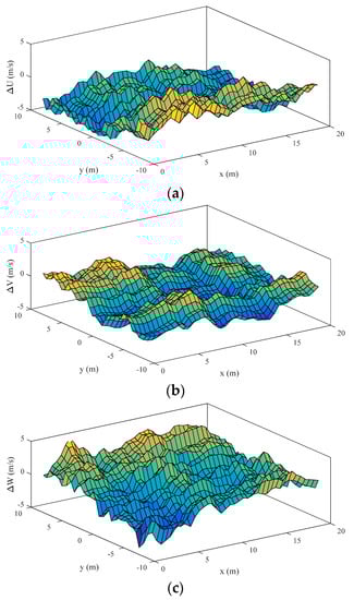
Figure 3.
A slice of turbulence components on the horizontal plane. (a) Longitudinal turbulence component; (b) Lateral turbulence component; (c) Vertical turbulence component.
Figure 4 presents the comparison between the simulated and theoretical correlation coefficients over the turbulence field, where and are the autocorrelation coefficients between the longitudinal, lateral, and vertical turbulence components, respectively. The longitudinal and lateral turbulence components present a stronger correlation than the vertical one, which is in accordance with the results in Figure 3. The simulated correlation coefficients along all three directions agree well with the theoretical results.
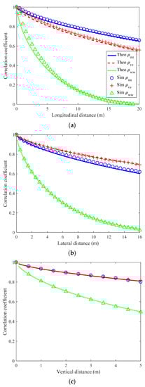
Figure 4.
Comparison between simulated and theoretical correlation coefficients. (a) Along longitudinal direction; (b) Along lateral direction; (c) Along vertical direction.
Figure 5 presents a comparison between simulated and theoretical turbulence spectra at a chosen point. It can be seen that the time histories of turbulence components experienced by a point in the turbulence field take the theoretical spectral characteristics in the frequency range of interest of handling qualities (1~10 rad/s).
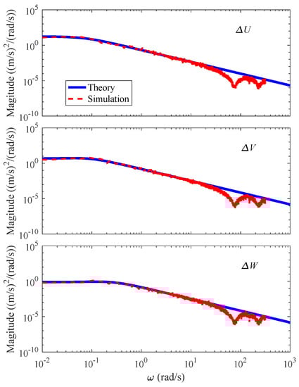
Figure 5.
Comparison between simulated and theoretical turbulence spectra at fuselage.
Simulations were also conducted for another wind condition with m/s, m, and m over a city center. The turbulence field grids are set to the same structure as above. Figure 6 shows the comparison between the simulated and theoretical correlation coefficients along lateral direction and Figure 7 presents the comparison between simulated theoretical spectra of vertical turbulence component at fuselage. It can be seen that both simulated correlation coefficients and spectra are in good agreement with the theoretical von Kármán model, demonstrating the performance of the proposed turbulence model over different terrains.
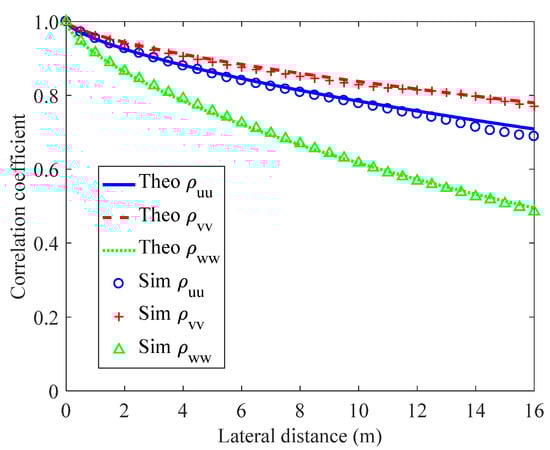
Figure 6.
Comparison between simulated and theoretical correlation coefficients along lateral direction for flight over a city center.
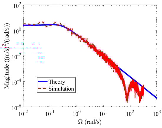
Figure 7.
Comparison between simulated and theoretical spectra of vertical turbulence component at fuselage for flight over a city center.
Finally, simulations were conducted with two different grid intervals to investigate the mesh convergence characteristics of the proposed model. The wind condition is set with m/s, m, and m to simulate turbulence over a city center. The turbulence field is set with m, m, and m. The lateral and vertical grid intervals are set with m, while the longitudinal grid interval is set with and 2 m, respectively. Figure 8 shows the comparison between simulated and theoretical spectra of vertical turbulence component at fuselage with different grid intervals. It is shown that simulated spectra agree well with the theoretical results at the low frequency range. However, the simulated spectra begin to collapse at a smaller frequency point from 36.4 rad/s to 18.2 rad/s as the grid interval increases from 1 m to 2 m, respectively. This is due to the fact that the turbulence samples of an aircraft are updated by the time step and thus the Nyquist frequency , as the aircraft is flying through the turbulence field with the relative speed To obtain high-fidelity simulation results in the frequency range in which handling qualities is of interest (about 1–10 rad/s), the grid interval should be small enough that for turbulence sample update is at least double than the upper threshold (10 rad/s).
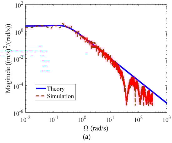
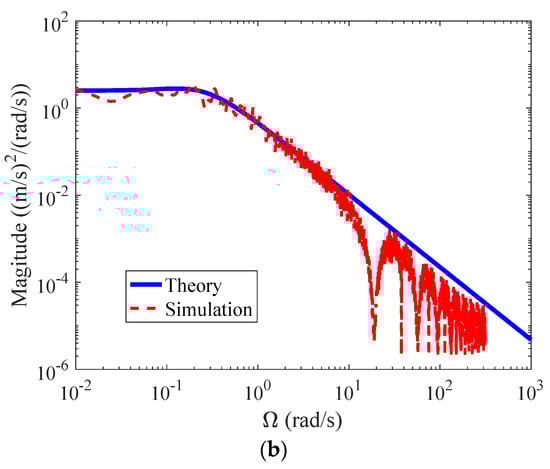
Figure 8.
Comparison between simulated and theoretical spectra of vertical turbulence component at fuselage with different grid intervals. (a) ; (b) .
3. Simulation Environment
Figure 9 shows the simulation scheme for rotorcraft maneuvering flight in turbulent wind. The turbulent wind vector is first calculated from the turbulence model and then transferred to a high-order nonlinear rotorcraft flight dynamics model including turbulence dynamics. The pilot model plans a desired trajectory complying with the mission task requirement. The control from the pilot model after comparing the desired trajectory and the rotorcraft motions is generated for stabilization and guidance. These consist of the whole framework for rotorcraft maneuvering flight in turbulent wind implemented in this paper.
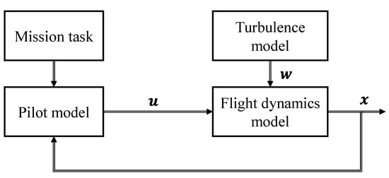
Figure 9.
Simulation scheme for rotorcraft maneuvering flight in turbulent wind.
3.1. Flight Dynamics Model
A generic UH-60A rotorcraft model [18,19,20] is used for investigation in this paper. The model is formulated with both rigid body dynamics and high-order main rotor dynamics. A three-state dynamic inflow model is used to simulate the main rotor inflow dynamics. The aerodynamic forces and moments of the main rotor are determined with blade element theory. The airfoil lift and drag coefficients of the blade elements are obtained with interpolation to wind tunnel test data. The main rotor blades are assumed to be rigid bodies. The rigid flapping and lagging motions of each blade are derived from aerodynamic and inertial moment equilibrium at the hinge. The elastic torsional degree of freedom of the blade is modeled empirically as a dynamic twist affecting equally each of the rotor blades. The impact of atmospheric turbulence on the vehicle is considered by superimposing the turbulent wind components directly on the local inflow components of each aerodynamic surface (including main rotor blade elements, fuselage, horizontal stabilator, vertical fin, and tail rotor). A Stability Augmentation System (SAS) is developed that resembles the SAS of the UH-60A rotorcraft [18], as shown in Appendix A. The SAS functions provide three-axis rate damping and lagged rate damping (pseudo attitude hold). The control authority of each channel is limited to percent of total control travel in pitch, roll, and yaw. The simplified transfer functions for roll, pitch, and yaw channels are given below, respectively,
where , , and are the SAS control signals for roll, pitch, and yaw channels, and and are the roll, pitch, and yaw rates.
The incorporated turbulent wind model and flight dynamics model can be expressed as,
where is the state vector of motion,
where are the linear velocity components and angular rates of the fuselage. are the Euler angles. are the flapping angular rates and angles of the four rigid blades. are the lagging angular rates and angles. are the blade tip dynamic torsion angle and angular rate. are the main rotor induced velocities. is the tail rotor induced velocity. and are the delayed fuselage downwash and sidewash components, respectively. is a rotorcraft’s four conventional controls,
where is collective input, is lateral cyclic stick input, is longitudinal cyclic stick input, and is pedal input. is the turbulence disturbances on the aircraft aerodynamic surfaces,
where are the instantaneous wind components at the th segment of, th blade of the main rotor, are the instantaneous wind components at the fuselage, are the instantaneous wind components at the horizontal stabilator, are the instantaneous wind components at the vertical fin, and are the instantaneous wind components at the tail rotor.
The flight dynamics model has been validated by comparing the trim results and frequency responses to cockpit controls against flight test data. More details about the model validation can be found in Refs. [6,7,8,20].
3.2. Pilot Model
A pilot model is designed to control the flight dynamics model to perform maneuvering flight in turbulent wind. The proposed pilot control strategy is presented in Figure 10, consisting of a stabilization component, a trajectory tracking component, and a trajectory planning component. The stabilization control component, modelled by the structural pilot model from Hess’ research [21,22], is used in the inner loop to stabilize rotorcraft attitudes and vertical acceleration. The attitude angles , , angular rates , and the vertical acceleration are used as input signals to produce the four conventional cockpit controls , , , and . The pilot model also tracks the desired attitudes ,, and vertical acceleration when performing maneuvering flight. The control efforts are defined by the crossover frequencies of the pilot-vehicle open loop system in each control channel. The crossover frequencies for all four control channels are 2 rad/s, which is a representative value of high-gain pilot control activity derived from flight test data [21].
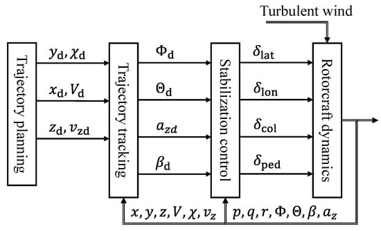
Figure 10.
Control strategy for rotorcraft maneuver in turbulent wind.
The trajectory tracking component is to control a vehicle to track the desired trajectory. The preview control law by Ji et al. [23] is employed to produce the desired attitudes ,, and vertical acceleration
where are the control gains to track the desired horizontal velocity , course angle , and vertical velocity . are the desired horizontal velocity, course angle, and vertical velocity at the time point . are the horizontal velocity, course angle, and vertical velocity at the current time . are the control gains for position control. are the errors between desired and corresponding position coordinates
where are the desired position coordinates in the NED axes, are the position coordinates in the NED axes, and is the yaw attitude.
The pilot gains are designed to obtain desired crossover frequencies for control of horizontal speed, course angle, and vertical velocity. According to the guidance for multi-loop pilot models [22,24], the crossover frequencies are chosen to be 0.67 rad/s, 1/3 of the inner-loop crossover frequencies. The control gains are designed to obtain desired crossover frequencies for longitudinal, lateral, and vertical position control, and the associated crossover frequencies are 0.13 rad/s.
The trajectory planning component in Figure 10 functions as planning a desired trajectory following a maneuvering task. An Approach-to-Hovering task is chosen herein for example to demonstrate the trajectory planning method. The flight path of this task consists of three phases, as presented in Figure 11, where and are the initial and final position coordinates in the NED axes for the flight phase, and is the glide angle. The first phase is a Level-to-Descent flight, starting with a steady level flight at the time , followed by a steady descent flight at the time for a Decelerating-Approach task [25] in the second flight phase. The initial altitude is 121.92 m (400 ft) for a medium-height approach [26]. The flight speed remains constant at 51.45 m/s (100 knots) and the final glide angle is 4 degrees to meet the requirements of the Decelerating-Approach task. The final altitude is selected to 109.73 m (360 ft). The initial and final conditions are summed as follows
where and are the initial and final flight speeds, are the initial velocity components in the NED axes, are the final velocity components in the NED axes. The acceleration profiles are programmed using trigonometric functions to smoothly transition from the initial condition to the final
where and are the amplitudes and are the angular frequencies. The following constraints are obtained by integrating the acceleration components with respect to time to solve the parameters , and ,
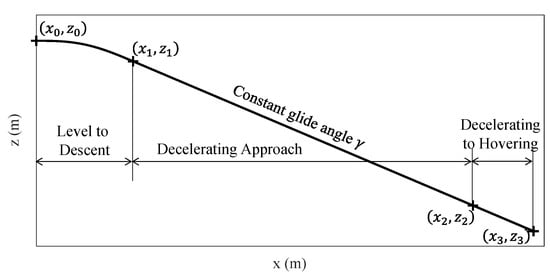
Figure 11.
Flight path for Approach-to-Hovering task.
The second phase is the Decelerating-Approach task defined in the ADS-33E [25]. It starts on a 4-degree glideslope at the speed of 51.45 m/s (100 knots), and then takes a manual deceleration to 12.86 m/s (25 knots) at a height of 15.24 m (50 ft). The flight condition at the time is summed as
where is the flight speed, and are the velocity components in the NED axes. The acceleration profiles are programmed by
where is the amplitude and is the angular frequency. The following constraints are obtained by integrating the longitudinal acceleration with respect to time to get the parameters and ,
where and .
The final phase is a Decelerating-to-Hovering task following the last phase and ending up in a hovering state at the altitude of 9.14 m (30 ft)
where and are the velocity components in the NED axes. The acceleration profiles are
where are the amplitudes and the are the angular frequencies. The following constraints are obtained by integrating the acceleration components with respect to time to solve the parameters and ,
3.3. Validation of Simulation Model
A position-hold task in a turbulent wind environment was conducted to provide an overview of the fidelity level for the UH-60 rotorcraft adopted in this paper by comparison with flight test data. The flight test was conducted with the rotorcraft headed into the leeward turbulence of a hangar with a speed of 11.6 m/s and at a height of 12.2 m [9]. Two turbulence models were used to simulate the suburban turbulent wind environment for comparison between the proposed turbulence model and the CETI model. The turbulence environment is set with m/s, m, and m for the proposed turbulence model. The length of the turbulence field is 20 m, the width is 16.5 m, the height is 5 m, and the girds are set with the interval of 0.5 m along with all three directions. As a result, turbulence components are simulated at grid nodes. As to the CETI model, the wind speed and flight altitude are set as the same as above, the integral scale length is 16.4 m, and the turbulence intensity is 1.37 m/s [9]. Both simulations were conducted using a desktop computer with an Intel(R) Core(TM) I7-7700K 4.20 GHz CPU.
Figure 12 shows the comparison results of simulated pilot controls and rotorcraft responses in turbulence against the flight test data. Only roll, pitch, yaw, and heave rate responses are compared due to the availability of flight test data. It can be observed that both simulated pilot controls and rotorcraft responses agree well among the flight test data and the two different turbulence models. The computational cost, defined as the ratio between the CPU time used for simulation and the simulation time, is 54.04% for the proposed turbulence model and 4.59% for the CETI model. Although the CETI model is much more efficient, it is not feasible for simulations with varied flight altitude and speed. The advantage of the proposed turbulence model is suitable for real-time simulation of rotorcraft maneuvering flight in turbulence.
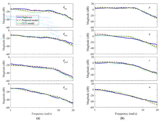
Figure 12.
Comparison of simulated pilot controls and rotorcraft responses in turbulence against flight test data. (a) Pilot controls; (b) Rotorcraft responses.
4. Investigation of Rotorcraft Maneuvering Flight in Turbulence
The Approach-to-Hovering task now is simulated in the turbulent wind environment to investigate the effect of varied flight conditions on piloted Handling Qualities Rating (HQR) for rejection of atmospheric turbulence. The flight trajectory and pilot model are set following the procedures in Section 3.2. Three wind conditions are considered as shown in Table 1. The first case represents a light wind condition with a low level of turbulence over a relatively smooth terrain [27], the second case is a strong wind condition with strong turbulence due to the increased wind speed over a smooth terrain, and the third case is a light wind condition with strong turbulence due to the rough terrain. The winds are all from North and the same intermediate height is used for determination of the integral length scales of turbulence. The moving spatial turbulence model is set with the same geometry and grids as the preceding section.

Table 1.
Simulated wind conditions.
The piloted HQR is measured by calculating the control attack parameter, which is defined as the ratio of the peak rate of control displacement () to the magnitude of the change in the control displacement () [28]
High attack values indicate small and rapid control deflections while a low value indicates large and slow control deflections. Using the control attack concept, the attack activity rate () metric defined in [29] is adopted to characterize the pilot control activity. The metric is defined as the ratio of the total number of that the pilot applies a particular control (>a threshold value) to the period of the task. The threshold value in this paper is selected as 2.5% of the full control range to capture ‘productive’ control inputs accounting for guidance and stabilization control activity [30]. The control activity rate () indicates the average ‘busyness’ metric of the task, but it masks local peaks in pilot control activity. However, pilots assign the level of HQR based on the most challenging phase of a task rather than the average. To identify the phase(s) within the task where a pilot is working hardest, Memon et al. [30] extended the metric to a time-varying localized attack activity rate (). The method includes the formulation of a control segmentation approach using a moving 5-s window with 2.5-s overlap between windows
where is the window size and is the total number of during a time segment of seconds around the time . Furthermore, a combined time-varying attack activity rate () is developed to correlate subjective pilot assessments. It is defined as the weighted sum of all controls’ with the corresponding fraction of the total control attacks in that axis
where corresponds to the four control channels (lateral, longitudinal, collective, and pedal), and is the time-varying total attack number in all four control channels
The flight test results indicated that the boundary for Level 1 HQR was 0.7 Hz and for Level 2 was 2.3 Hz, but the boundaries from ground simulators were 0.6 Hz for Level 1 and 1.3 Hz for Level 2 [30]. This paper selects the intermediate values of 0.65 Hz for Level 1 HQR and 1.8 Hz for Level 2.
Figure 13 and Figure 14 present the time profiles of desired velocities and wind conditions. The task is performed with the flight speed decelerating from 52 m/s to zero. The flight altitude reduces from 122 m to 9 m, resulting in decreased wind speed and increased turbulence intensities. Compared with Case 1, the rotorcraft experiences stronger wind speed and turbulence in Case 2 and similar wind speed but stronger turbulence in Case 3.
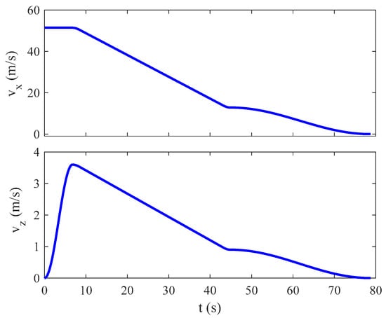
Figure 13.
Time profiles of desired velocities of aircraft.
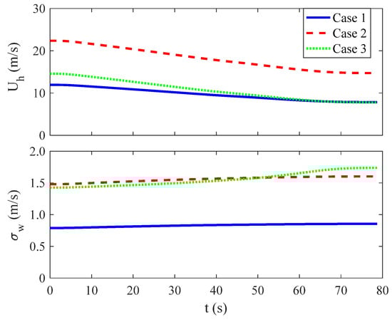
Figure 14.
Time profiles of wind speed and vertical turbulence intensity.
Figure 15 shows the time profiles of pilot controls for the Case 1 wind condition with SAS off, where the operation between adjacent control peaks marked with the sign ‘+’ represents one attack. It is observed that the pilot lowers down the collective lever and pulls back the cyclic stick to initiate deceleration at 6.6 s. The pilot applies the most aggressive controls in the longitudinal and vertical channels during 10–20 s, which is the most severely affected moment by turbulence, indicated by the densest control peaks. Then, the number of control peaks decreases with the decreased aircraft and wind speeds.
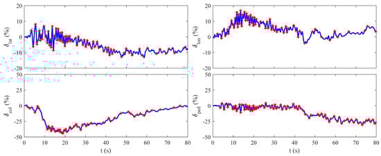
Figure 15.
Time profiles of pilot controls for Case 1 with SAS off.
The time-varying attack activity rates () for four control channels were estimated by Equation (50) and are presented in Figure 16. A total of 100 simulation runs were conducted for the case to enhance the trend pattern of with the averages of for each control channel. The results show that the piloted HQR reaches the worst during 10–20 s, consistent with the most aggressive pilot controls in the same period shown in Figure 15. After then, the pilot control activity in each channel decreases with the decreased flight speed as shown in Figure 13, which is in accordance with the rotorcraft response characteristics to turbulence with flight speed [1,6]. Finally, it seems that the pilot has the least control activity in the collective channel due to the vertical motion of the rotorcraft being least affected by turbulence.
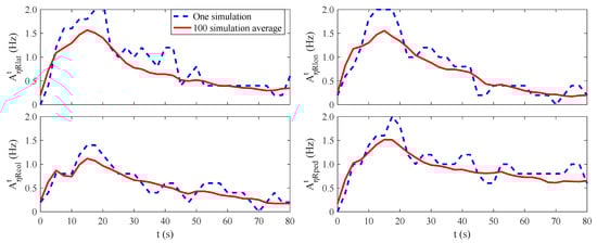
Figure 16.
Time-varying attack activity rates in four control channels for Case 1 with SAS off.
Figure 17 shows a full view of piloted HQRs in three wind conditions with SAS off, measured by the time-varying combined attack activity rates (). The results are averages from 100 simulation runs. It shows that the piloted HQR presents a similar tendency for three wind conditions. However, Case 1 presents the best HQR, Case 2 the worst due to stronger turbulence and larger airspeed resulting from larger wind speed, and Case 3 secondary due to stronger turbulence.
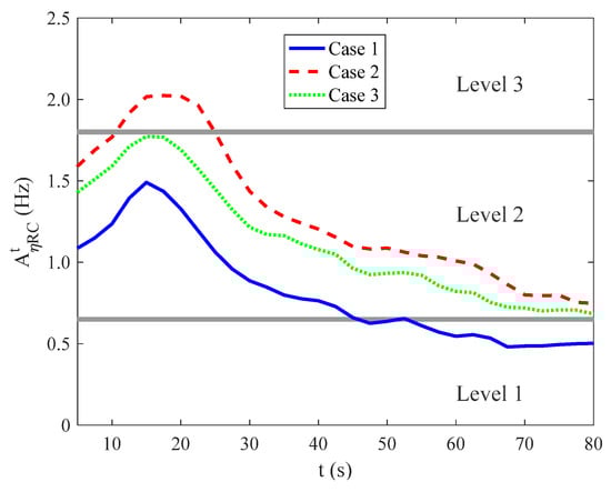
Figure 17.
Time-varying combined attack activity rates with SAS off.
Figure 18 shows the values with SAS on. Compared with those in Figure 17 with SAS off, the piloted HQR is significantly improved by the SAS throughout the flight.
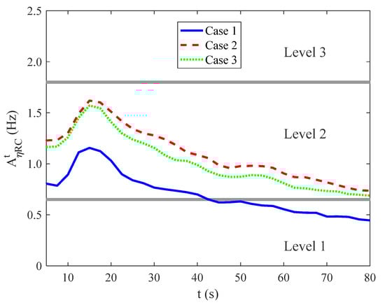
Figure 18.
Time-varying combined attack activity rates with SAS on.
5. Discussion
The above comparison results between theoretical prediction and simulation have demonstrated that the moving spatial turbulence model takes the spatial autocorrelation characteristics of turbulence components in all three directions. The comparison of turbulence spectra at fuselage indicates that the proposed model can produce turbulence components with desired spectral characteristics in the frequency range of interest for any point in the turbulence field. The good match in both pilot controls and rotorcraft responses to turbulence between simulation and flight test data proves that the turbulence model, not only on its own but also when integrated with the flight dynamics and pilot models, reaches a high level of predictability. Moreover, the proposed model only produces a local spatial turbulence field using highly efficient recursive algorithms, and it is suitable for simulation of rotorcraft maneuvering with varied flight speed and altitude.
An Approach-to-Hovering task was taken as an example to investigate the effect of varied flight speed and altitude on rotorcraft maneuvering in turbulence. The time profiles of pilot controls and time-varying attack activity rates in four control channels for Case 1 with SAS off indicated that the pilot operations were more susceptive to turbulence, and the pilot control activity was severely increased when performing aggressive controls. The comparison results using the time-varying combined attack activity rates for different wind conditions and rotorcraft configurations revealed that the turbulence model, being integrated into the simulation environment, predicted the expected effect of varied flight speed, wind speed, turbulence intensity, and SAS on piloted HQR for rotorcraft flight in turbulence. The turbulence model thus is applicable for rotorcraft maneuvering flight in turbulence with varied flight and wind conditions.
Continuing work will extend application of the proposed turbulence model to modeling complex turbulent wind environments, such as turbulence in a microburst or above a complex terrain.
6. Conclusions
This paper developed a moving spatial turbulence model to explore the effect of varied flight speed and turbulence intensity on piloted handling qualities and performance in a synthetic simulation environment. The Approach-to-Hovering task was simulated, and the pilot-assigned HQRs were analyzed using attack metrics. The following conclusions can be drawn:
- (1)
- The developed moving spatial turbulence model can produce a local turbulence field in which any point shows the desired spectral characteristics in the frequency range.
- (2)
- The turbulence model has been validated in a synthetic simulation environment, being integrated with a flight dynamics model and a pilot model. The results show that the model can accurately capture the frequency characteristics of pilot controls and rotorcraft responses to turbulence.
- (3)
- The simulation results indicate that pilot control activities are susceptive to the level of turbulence and the HQRs severely deteriorate when the maneuver is more aggressive. The results further have predicted the expected effect of varied flight speed, wind speed, turbulence intensity, and SAS on piloted handling qualities and control performance.
Author Contributions
Conceptualization, H.J., R.C. and L.L.; methodology, H.J., R.C. and L.L.; software, H.J.; validation, H.J.; formal analysis, H.J. and L.L.; investigation, H.J. and L.L.; resources, H.J.; data curation, H.J.; writing—original draft preparation, H.J.; writing—review and editing, L.L.; visualization, H.J.; supervision, L.L. and R.C.; project administration, H.J. and R.C.; funding acquisition, H.J. and R.C. All authors have read and agreed to the published version of the manuscript.
Funding
This research was supported by the National Natural Science Foundation of China, NO: 11902052; the Chongqing Science and Technology Commission (Bureau), NO: cstc2019jscx-msxmX0043; the National Key Laboratory of Science and Technology on Rotorcraft Aeromechanics, Nanjing University of Aeronautics and Astronautics, NO: JZX7Y201911SY004001; the Rotor Aerodynamics Key Laboratory, China Aerodynamics Research and Development Center, NO: RAL20190201).
Institutional Review Board Statement
Not applicable.
Informed Consent Statement
Not applicable.
Data Availability Statement
Not applicable.
Conflicts of Interest
The authors declare no conflict of interest.
Appendix A. Digital SAS of UH-60A Rotorcraft
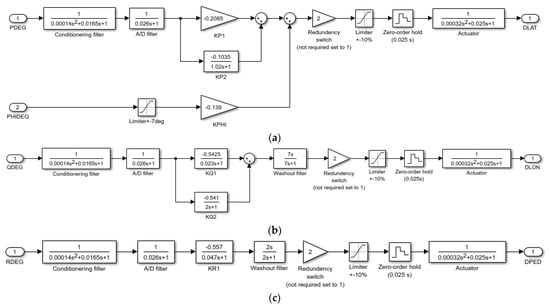
Figure A1.
Digital SAS of the UH-60A rotorcraft reproduced from [18]. (a) Roll channel; (b) Pitch channel; (c) Yaw channel.
References
- Ji, H.; Chen, R.; Lu, L.; White, M.D. Pilot workload investigation for rotorcraft operation in low-altitude atmospheric turbulence. Aerosp. Sci. Technol. 2021, 111, 106567. [Google Scholar] [CrossRef]
- Campbell, C.W.; Sanborn, V.A. A Spatial Model of Wind Shear and Turbulence. J. Aircr. 1984, 21, 929–935. [Google Scholar] [CrossRef]
- Robinson, J.E.; Weber, T.L.; Miller, D.G. Real-Time Simulation of Full-Field Atmospheric Turbulence for a Piloted Rotorcraft Simulation. In Proceedings of the 50th Annual Forum of the American Helicopter Society, Washington, DC, USA, 11–13 May 1994. [Google Scholar]
- Dang, Y.Y.; Gaonkar, G.H.; Prasad, J.V.R. Parallel Methods for Turbulence Simulation and Helicopter Response Prediction. J. Am. Helicopter Soc. 1996, 41, 219–231. [Google Scholar] [CrossRef]
- McFarland, R.E.; Duisenberg, K. Simulation of Rotor Blade Element Turbulence; NASA TM-108862; National Aeronautics and Space Administration: Washington, DC, USA, 1995. [Google Scholar]
- Ji, H.; Chen, R.; Li, P. Distributed Atmospheric Turbulence Model for Helicopter Flight Simulation and Handling-Quality Analysis. J. Aircr. 2017, 54, 190–198. [Google Scholar] [CrossRef]
- Ji, H.; Chen, R.; Li, P. Analysis of Helicopter Quality in Turbulence with Recursive von Kármán Model. J. Aircr. 2017, 54, 1631–1639. [Google Scholar] [CrossRef] [Green Version]
- Ji, H.; Chen, R.; Li, P. Distributed Turbulence Model with Accurate Spatial Correlations for Simulation of Helicopter Flight in Atmospheric Turbulence. J. Am. Helicopter Soc. 2019, 64, 042011. [Google Scholar] [CrossRef]
- Lusardi, J.A.; Tischler, M.B.; Blanken, C.L.; Labows, S.J. Empirically Derived Helicopter Response Model and Control System Requirements for Flight in Turbulence. J. Am. Helicopter Soc. 2004, 49, 340–349. [Google Scholar] [CrossRef]
- Seher-Weiss, S.; Jones, M. Control Equivalent Turbulence Input Models for Rotorcraft in Hover and Forward Flight. J. Guid. Control Dyn. 2021, 44, 1517–1524. [Google Scholar] [CrossRef]
- Berger, T.; Lopez, M.J.S. Frequency Domain Identification of a Multi-Input Control Equivalent Turbulence Input Model. J. Guid. Control Dyn. 2022, 45, 15–27. [Google Scholar] [CrossRef]
- Anderson, D. Helicopter Vibration Induced by Highly Structured Turbulence. J. Am. Helicopter Soc. 2003, 48, 244–252. [Google Scholar] [CrossRef]
- Huecas, S.H.; White, M.D.; Barakos, G. A Turbulence Model for Flight Simulation and Handling Qualities Analysis based on a Synthetic Eddy Method. J. Am. Helicopter Soc. 2022. [Google Scholar] [CrossRef]
- Liu, X.; Abà, A.; Capone, P.; Manfriani, L.; Fu, Y. Atmospheric Disturbance Modelling for a Piloted Flight Simulation Study of Airplane Safety Envelope over Complex Terrain. Aerospace 2022, 9, 103. [Google Scholar] [CrossRef]
- Etkin, B. Flight in Turbulent Atmosphere. In Dynamics of Atmospheric Flight; John Wiley and Sons, Inc.: New York, NY, USA, 1972; pp. 529–563. [Google Scholar]
- Ascher, U.M.; Chen, G. A First Course in Numerical Methods; Society for Industrial and Applied Mathematics: Philadelphia, PA, USA, 2011; pp. 104–107. [Google Scholar]
- Anonymous. Characteristics of the Wind Speed in the Lower of the Atmosphere near the Ground: Strong Winds (Neutral Atmosphere); Technical Report ESDU 72026; Engineering Sciences Data Unit Ltd.: London, UK, 1972. [Google Scholar]
- Howlett, J.J. UH-60A Black Hawk Engineering Simulation Program; NASA CR-166309; National Aeronautics and Space Administration: Washington, DC, USA, 1981. [Google Scholar]
- Kim, F.D. Formulation and Validation of High-Order Mathematical Models of Helicopter Flight Dynamics. Ph.D. Dissertation, University of Maryland, College Park, MD, USA, 1991. [Google Scholar]
- Ji, H.; Chen, R.; Li, P. Rotor-State Feedback Control to Alleviate Pilot Workload for Helicopter Shipboard Operations. J. Guid. Control Dyn. 2017, 40, 3088–3099. [Google Scholar] [CrossRef]
- Hess, R.A.; Zeyada, Y.; Heffley, R.K. Modeling and Simulation for Helicopter Task Analysis. J. Am. Helicopter Soc. 2002, 47, 243–252. [Google Scholar] [CrossRef]
- Hess, R.A.; Marchesi, F. Analytical Assessment of Flight Simulator Fidelity Using Pilot Models. J. Guid. Control. Dyn. 2009, 32, 760–770. [Google Scholar] [CrossRef]
- Ji, H.; Chen, R.; Lu, L.; White, W.D. Advanced Pilot Modeling for Prediction of Rotorcraft Handling Qualities in Turbulent Wind. Aerosp. Sci. Technol. 2022, 123, 107501. [Google Scholar] [CrossRef]
- Lu, L.; Jump, M. Multiloop Pilot Model for Boundary-Triggered Pilot-Induced Oscillation Investigations. J. Guid. Control Dyn. 2014, 37, 1863–1879. [Google Scholar] [CrossRef]
- ADS-33E (PRF); Handling Qualities Requirements for Military Rotorcraft. U.S. Department of Defense: Washington, DC, USA, 2000.
- Bachelder, E.; Berger, T.; Godfroy-Cooper, M.; Aponso, M. Pilot Workload and Performance Assessment for a Coaxial-Compound Helicopter and Tiltrotor during Aggressive Approach. In Proceedings of the Vertical Flight Society’s 77th Annual Forum & Technology Display, Virtual, 10–14 May 2021. [Google Scholar]
- MIL-F-8785C; Flying Qualities of Piloted Airplanes. U.S. Department of Defense: Washington, DC, USA, 1980.
- Padfield, G.D.; Jones, J.P.; Charlton, M.T.; Howell, S.E.; Bradley, R. Where Does the Workload Go when Pilots Attack Manoeuvres? An Analysis of Results from Flying Qualities Theory and Experiment. In Proceedings of the 20th European Rotorcraft Forum, Amsterdam, The Netherlands, 4–7 October 1994. [Google Scholar]
- Perfect, P.; Gubbels, A.W.; White, M.D.; Padfield, G.D.; Gubbels, A.W. Rotorcraft Simulation Fidelity: New Methods for Quantification and Assessment. Aeronaut. J. 2013, 117, 235–282. [Google Scholar] [CrossRef]
- Memon, W.A.; White, M.D.; Padfield, G.D.; Cameron, N.; Lu, L. Helicopter Handling Qualities: A Study in Pilot Control Compensation. Aeronaut. J. 2022, 126, 152–186. [Google Scholar] [CrossRef]
Publisher’s Note: MDPI stays neutral with regard to jurisdictional claims in published maps and institutional affiliations. |
© 2022 by the authors. Licensee MDPI, Basel, Switzerland. This article is an open access article distributed under the terms and conditions of the Creative Commons Attribution (CC BY) license (https://creativecommons.org/licenses/by/4.0/).