Dynamic Jellyfish Search Algorithm Based on Simulated Annealing and Disruption Operators for Global Optimization with Applications to Cloud Task Scheduling

Abstract

This paper presents a novel dynamic Jellyfish Search Algorithm using a Simulated Annealing and disruption operator, called DJSD. The developed DJSD method incorporates the Simulated Annealing operators into the conventional Jellyfish Search Algorithm in the exploration stage, in a competitive manner, to enhance its ability to discover more feasible regions. This combination is performed dynamically using a fluctuating parameter that represents the characteristics of a hammer. The disruption operator is employed in the exploitation stage to boost the diversity of the candidate solutions throughout the optimization operation and avert the local optima problem. A comprehensive set of experiments is conducted using thirty classical benchmark functions to validate the effectiveness of the proposed DJSD method. The results are compared with advanced well-known metaheuristic approaches. The findings illustrated that the developed DJSD method achieved promising results, discovered new search regions, and found new best solutions. In addition, to further validate the performance of DJSD in solving real-world applications, experiments were conducted to tackle the task scheduling problem in cloud computing applications. The real-world application results demonstrated that DJSD is highly competent in dealing with challenging real applications. Moreover, it achieved gained high performances compared to other competitors according to several standard evaluation measures, including fitness function, makespan, and energy consumption.

1. Introduction

Every day, new and complex optimization problems arise in fields such as mathematics, industry, and engineering [1]. When the problems became more complex, traditional optimization approaches were discovered with high computing costs and they were trapped in local optima while solving them [2]. As a result, scientists have been looking for new techniques to address these problems [3]. Metaheuristic algorithms are promising solutions proposed by drawing inspiration from herd animals’ food-finding habits or natural occurrences. Metaheuristic (MH) algorithms have many benefits, including the ability to resist local optima, use a gradient-free mechanism, and provide rational solutions regardless of problem structure [4].

Mathematical optimization is the process of locating an item within an accessible domain for a given problem that has a maximum or minimum value [5]. The advancement of optimization methods is critical since optimization problems arise in different fields of analysis. The majority of traditional optimization approaches are deterministic and rely on derivative knowledge [6]. However, in real life, determining the optimal values of a problem is not always feasible [7]. Because of their derivative-free behavior and promising optimization ability, MH techniques are becoming increasingly popular. Other benefits of these approaches include flexibility, ease of execution, and the avert ability to skip local optima [8].

Exploration and exploitation of the MH technique are two main methods used in metaheuristics [9]. Exploration refers to the opportunity to discover or visit new areas of the solution space. In contrast, exploitation refers to retrieving valuable knowledge about nearby regions from the found search domain. The balance between manipulation and discovery determines the consistency of the solutions found by any MH. These algorithms (i.e., MH), look for a single candidate agent or a set of agents. Single agent-oriented approaches are those that are based on a single candidate agent, whereas population-based approaches are those that are based on a group of candidate solutions. MH are made to look like natural phenomena. MH techniques can be divided into three categories depending on their source of inspiration: swarm intelligence-based algorithms, evolutionary algorithms, and physics-based algorithms.

Swarm intelligence has risen to prominence in the world of nature-inspired strategies in recent years [10]. It is also utilized to address real-life optimization problems and is focused on the mutual actions of swarms or colonies of animals [11]. Swarm-based optimization algorithms use the collaborative trial and error approach to find the optimal solution. The Arithmetic Optimization Algorithm (AOA) [10], the Aquila Optimizer (AO) [12], and the Barnacles Mating Optimizer (BMO) [13] are well-known methods in this category. Thus, many complicated optimization problems have been solved using this class of optimization algorithm, such as scheduling problems [14].

Recently, a new swarm-based optimization technique has been proposed which named is named the Jellyfish Search Algorithm (JSA) [15]. This algorithm emulates the behaviour of a jellyfish swarm in nature. In accordance with the characteristics of JSA, it has been applied to solve different sets of optimization problems. For example, JSA has been used to determined the optimal solution of global benchmark functions in [15] and its efficiency over other metaheuristic (MH) techniques has been established. Gouda et al. [16] proposed an alternative method for estimating the parameters of the PEM fuel cell. In [17], a multi-objective version of JSA is proposed and it has been applied to solve multiple objective engineering problems. In [18], the JSA was implemented to solve the spectrum defragmentation problem and it showed better performance compared to other methods. Chou et al. [19] presented a time-series forecasting method for energy consumption. This method was compared with other teaching-learning-based optimization (TLBO) and symbiotic organism search (SOS) algorithms. The results of JSA are better than those algorithms. In addition, JSA was applied to other fields such as video watermarking [20].

In previous applications of JSA, its ability to solve different optimization problems has been observed. However, it still suffers from some drawbacks that can affect its performance. For example, it requires more improvement in its ability to balance between the exploration and exploitation phases during the searching process. This motivated us to propose an alternative version of JSA to avoid the limitations of conventional JSA and to apply it as a global optimization technique.

The proposed developed version of JSA is called DJSD—dynamic differential annealed technique. The proposed DJSD method integrated the Jellyfish Search Algorithm operators with active differential annealed optimization [21] and the disruption operator to gain the advantages of both approaches. The proposed method is evaluated using various benchmark problems (i.e., classical benchmark). The proposed approach’s performance is analyzed and compared with other methods to solve the same problems. The results proved that the presented method is better than other comparative approaches, and it found new best solutions for several test cases. In addition, it is extended by using it as a task scheduler technique in a cloud computing environment.

In conclusion, the following contributions are included in this paper:

• Enhancing the Jellyfish Search Algorithm using the concept of the dynamic annealed and disruption operator to improve its exploration and exploitation abilities during the searching process.
• Applying the developed method, named DJSD, as a global optimization method through evaluating it using different classical optimization benchmark functions against other well-known MH methods.
• Offering an alternative task scheduling method to address cloud task scheduling problems.

The remaining sections of this paper are organized as follows. Section 2 presents the background of the jellyfish optimization algorithm, the Simulated Annealing algorithm, and the disruption operator. Section 3 introduces the steps of the proposed method. The experimental results and discussions are presented in Section 4. Finally, Section 5 concludes the paper.

2. Background

2.1. Jellyfish Search Algorithm

In this section, the basic information of the Jellyfish Search Algorithm (JSA) [15] is given. In general, JSA simulates the behaviour of jellyfish that squeeze water out of their body to move; rising ocean temperatures cause the creation of swarms [15]. The ability of these species to appear almost anywhere in the ocean is due to their movements within a swarm and the ensuing ocean currents that form jellyfish blooms. Since the amount of food at jellyfish-friendly sites varies, the best location would be determined by comparing food proportions [15].

Following [15], the ideas underpinning the jellyfish optimization algorithm can be formulated as:

• JSA goes around the water looking for food and is drawn to areas with a higher supply of food.
• The time control mechanism regulates shifting among motion groups. Jellyfish either move inside the swarm or follow the ocean current.

The major steps of metaheuristic algorithms are exploitation and exploration. Exploration is the motion in an ocean current, while exploitation is the motion inside a jellyfish swarm and the time control mechanism that manages the swapping between them. To locate areas with optimal locations, the possibility of exploration exceeds that of exploitation at the beginning. However, over time, exploitation’s probability exceeds that of exploration; then, the jellyfish determine the best position within the known places.

2.1.1. Population Initialization

In most cases, jellyfish populations are initiated at random positions, and the slow convergence and propensity to get stuck in the local optima due to low population diversity are some drawbacks of this strategy [15]. Therefore, many chaotic maps, for example, the tent map, the Liebovitch map, and the logistic map, have been created to increase the composition of the initial population. A logistic map generates a larger initial population than random selection and has a lower risk of premature convergence [15].

$$X_{i+1}=\eta X_i(1-X_i),0\le X_0\le 1$$

(1)

where $X_0$ is a basic jellyfish population, $X_i$ denotes the logistically chaotic value of the jellyfish’s location i, $\eta =4.0$, $X_0\in (0,1),$ and $X_0\notin \{0.0,0.25,0.75,0.5,1.0\}$.

Since the earth is roughly spherical, a jellyfish that leaves the search domain’s boundaries would go back to the direct opposite limit. This mechanism is represented in Equation (2).

$$X_{i,d}^{\prime }=\left\{\begin{array}{cc}(X_{i,d}-U{B}_d)+L{B}_{d}if{X}_{i,d}>U{B}_d\hfill & \\ (X_{i,d}-L{B}_d)+U{B}_{d}if{X}_{i,d}<L{B}_d\hfill \end{array}\right.$$

(2)

where $X_{i,d}^{\prime }$ denotes the new value of $X_{i,d}$ at dimension d after checking the limits of the search space (i.e., $UB$ and $LB$).

2.1.2. Exploration Stage: Ocean Current

The jellyfish are drawn to the ocean current because it carries many nutrients; the ocean current’s direction ($T_O$) is calculated as:

$$T_O=\frac{1}{N}\sum _i{T}_{O_i}=\frac{1}{N}\sum (X_b-e_c{X}_i)=X_b-e_c\frac{\sum X_i}{N}=X_b-e_c\mu$$

(3)

where $T_O$ is determined by:

$$T_O=X_b-df,df=e_c\mu$$

(4)

In Equation (4), N is the number of jellyfish, $X_b$ is the best jellyfish in the swarm with the best fitness value, $e_c$ is the attraction’s governing factor, $\mu$ is the jellyfish’s average position, $df$ the distinction among the jellyfish’s current best position and the average position of all jellyfish. Based on the assertion that jellyfish have a regular spatial distribution in all directions, and a distance of $\pm \beta \sigma$, all jellyfish are likely to be found in the vicinity of the mean position, and the standard deviation of the distribution is $\sigma$.

$$df=\beta \times \sigma \times ran{d}^f$$

(5)

$$\sigma =\mu \times ran{d}^{\alpha }$$

(6)

So,

$$df=\mu \times \beta \times ran{d}^f\times ran{d}^{\alpha },df=\mu \times \beta \times rand$$

(7)

$$e_c=\beta \times rand$$

(8)

$$T_O=X_b-\beta \times rand\times \mu$$

(9)

The value of $X_i$ is updated using Equation (10).

$$X_i(t+1)=rand\times T_O+X_i\left(t\right)$$

(10)

Based on the definition of $T_O$, Equation (10) can be reformulated as:

$$X_i(t+1)=\mu \times rand\times (X_b-\beta \times rand)+X_i\left(t\right)$$

(11)

In Equation (11), the length of $T_O$ is related to $\beta >0$, which is a coefficient of distribution, and $T_O$ depends on the findings of the numerical experiment’s sensitivity analysis.

2.1.3. Exploitation Stage

Jellyfish move in swarms in passive and active motions (group A and group B, respectively). When the swarm is first forming, most jellyfish move in a group A pattern. They increasingly exhibit active motion over time, and passive activity is the movement of jellyfish that surround their positions with each jellyfish’s updated position being provided as follows.

$$X_i(t+1)=(U_b-L_b)\times \gamma \times rand+X_i\left(t\right)$$

(12)

where $U_b$ denotes the upper limit and $L_b$ represents the lower limit of the search domain, and $\gamma >0$ is the coefficient of motion.

According to the numerical results of experiments’ sensitivity analyses, it was obtained that $\gamma =0.1$. To emulate the active motion of jellyfish (j), more than one are chosen randomly and a vector is employed to determine the direction of motion from $X_i$ to $X_j$. Every $X_i$ in a swarm moves in the best direction to find the food using Equations (13)–(16), to mimic the motion direction and modify the jellyfish position.

$$step=rand\times Direction$$

(13)

$$step=X_i(t+1)-X_i\left(t\right)$$

(14)

$$Direction=\left\{\begin{array}{cc}{X}_j\left(t\right)-X_i\left(t\right)\hfill & ifFi{t}_i\ge Fi{t}_j,\hfill \\ X_i\left(t\right)-X_j\left(t\right)\hfill & ifFi{t}_i<Fi{t}_j\hfill \end{array}\right.$$

(15)

where $Fit$ is the fitness function of position X.

$$X_i(t+1)=step+X_i\left(t\right)$$

(16)

2.1.4. Time Control Mechanism (TCM)

In the beginning, passive motion is preferred. However, with time, active movement is favored to mimic this case; we use a time control mechanism to organize jellyfish travel between going inside a jellyfish swarm and following the ocean current. The TCM has a time control function $c\left(t\right)$ which is a time-varying random value that ranges from 0 to 1, and $c_o$ is a constant; Equation (17) represents the TCM.

$$c\left(t\right)=|2\times (1-{\displaystyle \frac{t}{t_{max}}})\times (rand-1)|$$

(17)

where $t_{max}$ stands for the maximum number of generations. $(1-c(t\left)\right)$ is the function simulating the move inside a swarm (passive or active motion); when $rand(0,1)>(1-c(t\left)\right)$, X exhibits a passive motion. Otherwise, X exhibits an active motion.

The complete steps of the jellyfish optimization algorithm are given in Algorithm 1.

Algorithm 1 Steps of jellyfish optimization algorithm

1: Determine initial parameters such as N number of solutions, $t_{max}$ total number of generations.  2: Construct population $X_i(i=1,2,\dots ,N)$ utilizing logistic chaotic map.  3: Compute fitness function ($Fi{t}_i$) for $X_i$.  4: Allocate the best solution $\left(X_b\right)$.  5: Set $t=1$.  6: repeat  7:     for $i=1$ to N do  8:         Update $c\left(t\right)$ according to Equation (17).  9:         if $c\left(t\right)\ge 0.5$ then 10:            (1) Update $T_O$ using Equation (9). 11:            (2) Update $X_i$ using Equation (11). 12:         else: 13:            if $rand>(1-c(t\left)\right)$ then 14:                (1) Update $X_i$ according to Equation (12). 15:            else: 16:                (2) Update the direction of $X_i$ according to Equation (15). 17:                (3) Update $X_i$ according to Equation (16). 18:         Check boundary conditions for $X_i$. 19:         Compute $Fi{t}_i$ for $X_i$ and update $X_b$. 20:     $t=t+1$. 21: until$t>t_{max}$. 22: Output: $X_b$.

2.2. Simulated Annealing Algorithm

The Simulated Annealing (SA) algorithm is a single-based solution optimization technique simulating the metallurgical annealing process [22,23].

The SA algorithm starts by generating a random solution with a starting value X and comes up with a new solution Y from its neighborhood. The fitness value for X and Y is calculated as the following step in SA, and if $Fit\left(Y\right)\le Fit\left(X\right)$, then $X=Y$. On the other hand, SA can replace X with Y even when Y’s fitness is not greater than X’s. This is determined by the probability (p), which is defined as follows:

$$p=e^{\frac{-\Delta E}{T}},$$

(18)

$$\Delta E=\frac{Cost\left(X\right)-Cost\left(Y\right)}{Cost\left(Y\right)}$$

(19)

where T stands for the temperature variable, which should start high and steadily decrease in value as iterations progress. The probability of adopting a new solution is denoted by p. The difference between the objective value of the suggested solution Y and the solution X objective value is called $\Delta E$. The SA algorithm is illustrated in Algorithm 2.

Algorithm 2 The SA method

Input: Initial temperature ($T_0$), D is the solution dimension and $t_{max}$ is the maximum number of generations. The initial solution is generated X. Compute the fitness value $Fit$ of X to evaluate its efficiency. Allocate the best solution $X_b=X$ and $Fit\left(X_b\right)=Fit\left(X\right)$. Allocate $t=1$ and $T=T_0$. while$t<t_{max}$do     Discover the neighbour Y for the X.     Compute $Fit\left(Y\right)$ for Y.     if $Fit\left(Y\right)<Fit\left(X_i\right)$ then         $X_i=Y$.     else         Update $\Delta =Fit\left(X_i\right)-Fit\left(Y\right)$.         if ($p\le r_5$) then            $X_i=Y$.     if $Fit\left(X_b\right)>Fit\left(X\right)$ then         $X_b=X$;     Set $t=t+1$. Output: $X_b$.

2.3. Disruption Operator

The preliminaries of the disruption operator ($D_{op}$) are described in this section. $D_{op}$ depends on the physical processes in astrophysics, where this rule supposes that when a set of gravitationally bound particles (with total mass m) is very close to a massive object (with mass M), then the group becomes torn apart [24]. The role in Equation (20) [24] can be used to implement this process:

$$D_{op}=\left\{\begin{array}{c}dis{t}_{i,j}\times \delta (\frac{-1}{2},\frac{1}{2})ifdis{t}_{i,best}\ge 1\\ 1+dis{t}_{i,best}\times \delta (\frac{-{10}^{-16}}{2},\frac{{10}^{-16}}{2})otherwise\end{array}\right.$$

(20)

where $dis{t}_{i,best}$ represents the Euclidean distance between the best solution and the $ith$ solution. $dis{t}_{i,j}$ denotes the Euclidean distance between the $ith$ solution and the nearest neighborhood ($jth$). Additionally, $\delta (a,b)$ represents a random value in domain $[a,b]$.

3. Developed Method

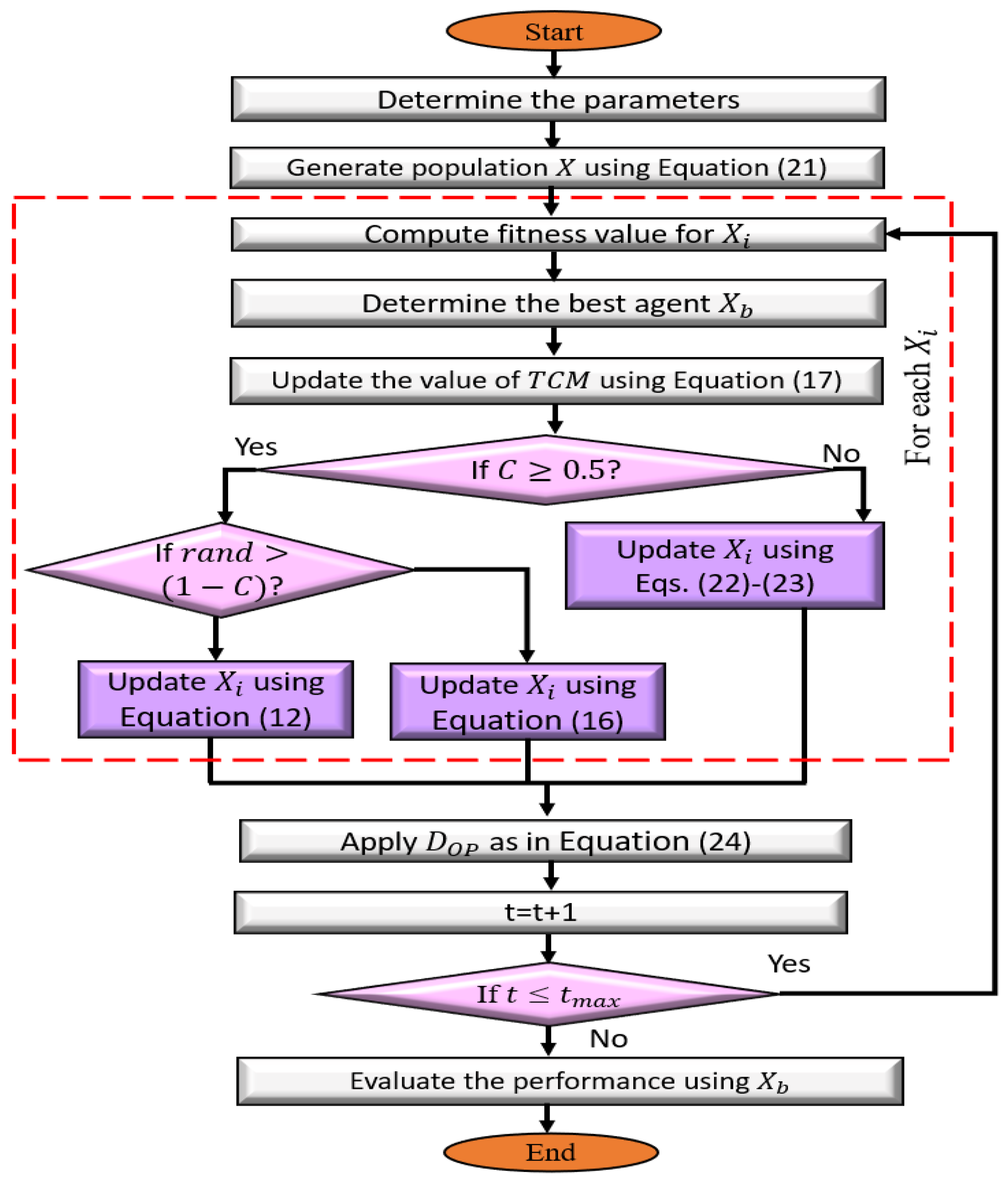
The framework of the presented DJSD method is illustrated in Figure 1. The improved DJSD aims to enhance the performance of the traditional JSA using dynamic differential Simulated Annealing and a disruption operator. Each of these techniques is applied to enhance the exploration and exploitation of JSA.

Figure 1. Schematic flowchart of the developed DJSD method.

The developed DJSD starts by producing the initial population then computing the fitness value for each agent inside this population. This is followed by determining the best agent that has the smallest fitness value. The following process updates the agents according to the time control mechanism (TCM) value, which determines whether the agents will be updated using an ocean current or jellyfish swarm. In the latter (i.e., the jellyfish swarm), the traditional operators of the JSA algorithm are applied to update the current agent. Otherwise, the competition between JSA operators, dynamic differential Simulated Annealing, and the $D_{op}$ are used to update the present agent. This is performed by updating the agents using either the traditional operators of the JSA in ocean current or the DJSD. Then, the mechanism of SA to decrease the probability of choosing a new agent as the temperature is reduced is applied. Finally, after updating the current population, the $D_{op}$ is used to improve the diversity of X.

3.1. Initial Stage

The developed DJSD starts at this point by constructing an initial population $\left(X_i\right)$ with N agents, and this is formulated as:

$$X_i=LB+rand(1,D)\times (UB-LB)$$

(21)

In Equation (21), $rand(1,D)$ stands for random D values. $LB$ and $UB$ refer to the limits of the search domain.

3.2. Updating Stage

At this stage, the DJSD starts updating the agents within the current population (X) by calculating the fitness value $Fi{t}_i$ for each agent $X_i$. The next step in DJSD is to allocate the best agent $X_b$, which has the best fitness value $Fi{t}_b$. Then the value of TCM is improved using Equation (17). In cases where $c\left(t\right)<0.5$, the operators of the jellyfish swarm are used to update $X_i$. Otherwise, the combination of ocean current, DJSD, and $D_{op}$ is used to enhance $X_i$. This is achieved based on the dynamic characteristics of the hammer during the search for the optimal solution. This represents a fluctuating parameter between the ocean current and the operator of SA. Hence, this process is formulated as:

$$X_i^{new}=\left\{\begin{array}{cc}{X}_i+rand\times X_b-\mu \times \beta \times rand\hfill & \mathrm{if}\mathrm{rem}(\mathrm{t},2)=1\hfill \\ (X_{r1}-X_{r2})+Xr\times f\hfill & \mathrm{if}\mathrm{rem}(\mathrm{t},2)=0\hfill \end{array}\right.$$

(22)

In Equation (22), $f\in [0,1]$ is random number and $rem$ represents the remaining mathematical function. $X_{r1},X_{r2}$ are random solutions chosen from the current population X, while $Xr$ denotes a random solution generated in the search space.

After that, the new value of $X_i$ (i.e., $X_i^{new}$) is accepted at temperatures elevated above low temperatures, and this is performed depending on the probability value p as in the traditional SA. This process is formulated as follows.

$$X_i=\left\{\begin{array}{cc}{X}_i^{new}\hfill & Fi{t}_i^{new}<Fi{t}_i\hfill \\ ApplyEquations\left(18\right)and\left(19\right)\hfill & Otherwise\hfill \end{array}\right.$$

(23)

The next step is to apply the $D_{op}$ operator to the current updated population X. However, this process takes more time, and this increases the computational time of the developed method. Accordingly, $D_{op}$ will be applied according to the following formula:

$$X_i=\left\{\begin{array}{cc}ApplyEquation\left(20\right)\hfill & rand>0.5\hfill \\ X_i\hfill & Otherwise\hfill \end{array}\right.$$

(24)

3.3. Terminal Stage

The stop conditions are checked within this stage; if they are not met, the updating stage is repeated. Otherwise, the best solution found so far ($X_b$) is returned.

4. Experimental Results and Discussion

In this section, the presented optimizer’s performance is evaluated using several experiments and comprehensive comparisons to demonstrate the algorithm’s abilities. The implemented experiments consist of a set of thirty classical benchmark functions. The results of the developed DJSD are compared with those of several metaheuristic optimizers including the whale optimization algorithm (WOA) [25], artificial ecosystem optimization (AEO) [26], the chimp optimization algorithm (Chimp) [27], the firefly algorithm (FA) [28], and the traditional JSA. The setting parameters for all comparison algorithms are given in Table 1. These values are chosen based on the original implementation of the algorithms. The considered algorithms are conducted 30 times with a population size of 30, and the maximum number of iterations per run is set to 1000. The experiments and analyses are executed using MATLAB R2018b on a machine equipped with an Intel Core i5 CPU and 4 GB RAM running under Windows 10 64-bit.

Table 1. The value of each parameter of compared methods.

Algorithm	Parameter Values
DJSD	$\gamma =0.1$, $\eta =4.0$
JSA	$\gamma =0.1$, $\eta =4.0$
AEO	$ran{d}_1,ran{d}_2,ran{d}_3,ran{d}_4\in [0,1]$
MFO	$a=\in [-2-1]$, Spiral factor $b=1$
FA	${\beta }_0=1$, ${\gamma }_{FA}\in [0.01-100]$, ${\alpha }_{FA}\in [0,1]$
Chimp	$a=[-1,1]$,   f decreased from $2\to 0$
WOA	$a=[0,2],b=1,l=[-1,1]$

4.1. Experimental Series 1: Mathematical Optimization Problems

The major objective of the current experimental series is to assess the ability of the developed method to determine the ideal solution for classical benchmark functions [29]. The description of these benchmark functions is given in Table 2. It is evident from the table that there are two types of functions, namely unimodal (UM) and multimodal (MM). The unimodal type (F1–F10) is used to assess the ability of the MH technique to find the solution inside a a single solution search space. Likewise, the multimodal type (F11–F30) is applied to test the capability of the MH method to find the optimal solution inside a search domain having more extreme solutions.

Table 2. Formulation of global problems.

ID	Formula of Function	$\mathbf{LW}$	$\mathbf{UW}$	${\mathbf{dim}}_{\mathit{W}}$	Type
F1	$f\left(x\right)={\sum }_{i=1}^n{x}_i^2$	−100	100	30	UM
F2	$f\left(x\right)={\sum }_{i=1}^n|x_i|+{\Pi }_{i=1}^n\left|x_i\right|$	−10	10	30	UM
F3	$f\left(x\right)={\sum }_{i=1}^n{\left({\sum }_{j-1}^i{x}_i\right)}^2$	−100	100	30	UM
F4	$f\left(x\right)=ma{x}_i\left\{\right|x_i|,1⩽i⩽n\}$	−100	100	30	UM
F5	$f\left(x\right)={\sum }_{i=1}^{n-1}[100{(x_{i+1}-x_i^2)}^2+{(x_i-1)}^2]$	−30	30	30	UM
F6	$f\left(x\right)={\sum }_{i=1}^n{\left([x_i+0.5]\right)}^2$	−100	100	30	UM
F7	$f\left(x\right)={\sum }_{i=1}^{n}i{x}_i^4+random[0,1]$	−1.28	1.28	30	UM
F8	$f\left(x\right)={\sum }_{i=1}^{n}i{x}_i^2$	−10	10	30	UM
F9	$f\left(x\right)={\sum }_{i=1}^{n}i{x}_i^4$	−1.28	1.28	30	UM
F10	$f\left(x\right)={\sum }_{i=1}^n{\left|x_i\right|}^{i+1}$	−1	1	30	UM
F11	$f\left(x\right)={\sum }_{i=1}^n-x_{i}sin\left(\sqrt{|x_i|}\right)$	−500	500	30	MM
F12	$f\left(x\right)={\sum }_{i=1}^n[x_i^2-10cos\left(2\pi x_i\right)+10]$	−5.12	5.12	30	MM
F13	$f\left(x\right)=-20exp(-0.2\sqrt{\frac{1}{n}{\sum }_{i=1}^n{x}_i^2})-exp\left(\frac{1}{n}{\sum }_{i=1}^{n}cos\left(2\pi x_i\right)\right)+20+e$	−32	32	30	MM
F14	$f\left(x\right)=\frac{1}{4000}{\sum }_{i=1}^n{x}_i^2-{\Pi }_{i=1}^{n}cos\left(\frac{x_i}{\sqrt{i}}\right)+1$	−600	600	30	MM
F15	$f\left(x\right)=\frac{\pi }{n}\{10si{n}^2\left(\pi y_1\right)+{\sum }_{i=1}^{n-1}{(y_i-1)}^2[1+10si{n}^2\left(\pi y_{i+1}\right)]+{(y_n-1)}^2\}+{\sum }_{i=1}^{n}u(x_i,10,100,4)$	−50	50	30	MM
	$u(x_i,a,k,m)=\left\{\begin{array}{cc}k{(x_i-a)}^m,\hfill & x_i>a\hfill \\ 0,\hfill & -a⩽x_i⩽a\hfill \\ k{(-x_i-a)}^m,\hfill & x_i<-a\hfill \end{array}\right.$
F16	$f\left(x\right)=0.1\{si{n}^2\left(3\pi x_1\right)+{\sum }_{i=1}^n{(x_i-1)}^2[1+si{n}^2(3\pi x_i+1)]+{(x_n-1)}^2[1+si{n}^2\left(2\pi x_n\right)]\}+{\sum }_{i=1}^{n}u(x_i,5,100,4)$	−50	50	30	MM
F17	$f\left(x\right)={\sum }_{i=1}^n{(x_i-1)}^2+[1+si{n}^2(3\pi x_i+1)]+si{n}^2\left(3\pi x_1\right)+|x_n-1|[1+si{n}^2\left(3\pi x_n\right)]$	−10	10	30	MM
F18	$f\left(x\right)={\sum }_{i=1}^n|x_{i}sin\left(x_i\right)+0.1x_i|$	−10	10	30	MM
F19	$f\left(x\right)=0.1n-(0.1{\sum }_{i=1}^{n}cos\left(5\pi x_i\right)-{\sum }_{i=1}^n{x}_i^2$	−1	1	30	MM
F20	$f\left(x\right)={\sum }_{i=1}^n{x}_i^2+{\left({\sum }_{i=1}^{n}0.5i{x}_i\right)}^2+{\left({\sum }_{i=1}^{n}0.5i{x}_i\right)}^4$	−5	10	30	MM
F21	$f\left(x\right)={\sum }_{i=1}^{n}0.5+\frac{si{n}^2(\sqrt[]{100x_{i-1}^2}+x_i^2-0.5)}{1+0.001{(x_i^2-2x_{i-1}{x}_i+x_i^2)}^2}$	−5	10	30	MM
F22	$f\left(x\right)=0.1si{n}^2\left(3\pi x_1\right)+{\sum }_{i=1}^{n-1}{(x_i-1)}^2(1+si{n}^2\left(3\pi x_{i+1}\right)+{(x_n-1)}^2(1+si{n}^2\left(3\pi x_n\right))$	−5	5	30	MM
F23	$f\left(x\right)={\sum }_{i=1}^n{\left({10}^6\right)}^{(i-1)/(n-1)}{x}_i^2$	−100	100	30	MM
F24	$f\left(x\right)={(-1)}^{n+1}{\Pi }_{i=1}^n\left(cos\left(x_i\right)\right)exp\left({\sum }_{i=1}^n{(x_i-\pi )}^2\right)$	−100	100	30	MM
F25	$f\left(x\right)=1-cos\left(2\pi \sqrt[]{{\sum }_{i=1}^n{x}_i^2}\right)+0.1\sqrt[]{{\sum }_{i=1}^n{x}_i^2}$	−100	100	30	MM
F26	$f\left(x\right)=0.5+\frac{si{n}^2\left(\sqrt[]{{\sum }_{i=1}^n{x}_i^2}\right)-0.5}{{(1+0.001\left({\sum }_{i=1}^n{x}_i^2\right))}^2}$	−100	100	30	MM
F27	$f\left(x\right)={(\frac{1}{500}+{\sum }_{j=1}^{25}\frac{1}{j+{\sum }_{i=1}^2{(x_i-a_{ij})}^6})}^{-1}$	−65.536	65.536	2	MM
F28	$f\left(x\right)={\sum }_{i=1}^{11}{[a_i-\frac{x_1(b_i^2+b_i{x}_2)}{b_i^2+b_i{x}_3+x_4}]}^2$	−5	5	4	MM
F29	$f\left(x\right)=4x_1^2-2.1x_1^4+\frac{1}{3}{x}_1^6+x_1{x}_2-x_2^2+4x_2^4$	−5	5	2	MM
F30	$f\left(x\right)={(x_2-\frac{5.1}{4{\pi }^2}{x}_1^2+\frac{5}{\pi }{x}_1-6)}^2+10(1-\frac{1}{8\pi })cos{x}_1+10$	−5	5	2	MM

Results and Discussions

The findings of DJSD and other peer algorithms in terms of solving classical global benchmark functions are given in Table 3, Table 4, Table 5 and Table 6. From Table 3, which illustrates the average of the fitness value, it is clear that DJSD outperforms other peer methods in most of the tested functions. More specifically, it achieves the smallest fitness value in eighteen functions, representing 60% of the total tested functions, followed by AEO and FA ranked in the second and third places, respectively. Conversely, the traditional JSA only provides better results than MFO, Chimp, and WOA.

Table 3. Average of fitness value obtained by each algorithm.

	DJSD	JSA	AEO	MFO	FA	Chimp	WOA
F1	0.00E+00	3.71E-61	0.00E+00	2800.05	3.46E-20	5.3E-102	4.7E-148
F2	0.00E+00	1.7E-25	5.5E-163	39.22343	2.82E-11	2.42E-59	6.3E-106
F3	0.00E+00	14.62956	0.00E+00	18238.91	3.72E-20	4.12E-83	3.33E-10
F4	0.00E+00	1.3E-36	3.5E-162	74.64607	1.4E-10	1.66E-39	2.88E-06
F5	0.02752	0.039121	21.7095	3205702	2.76E-13	1.850126	13.89417
F6	0.016425	1.72E-09	6.46E-07	3620.098	3.56E-20	0.000822	1.12E-06
F7	1.66E-05	0.00021	0.000425	0.143259	2.29E-05	0.000235	0.000737
F8	0.00E+00	6.6E-12	0.00E+00	660.0002	8.21E-22	6.5E-103	2.4E-153
F9	0.00E+00	1.17E-57	0.00E+00	3.435974	3E-47	1.7E-181	5.4E-230
F10	0.00E+00	3.1E-101	9.5E-297	3.11E-09	2.48E-15	9.23E-96	6.4E-141
F11	−1632.06	−953.103	−1295.09	−1358.43	−214.577	−217.608	−217.608
F12	0.00E+00	0.001876	0.00E+00	175.4167	0.00E+00	0.117139	0.00E+00
F13	8.9E-16	3.45E-15	8.9E-16	15.96415	1.23E-10	4.3E-15	2.59E-15
F14	0.00E+00	0.00E+00	0.00E+00	18.24552	0.012442	0.033193	0.007454
F15	0.018289	3.2E-10	4.06E-08	56.90585	1E-21	0.000577	2.61E-05
F16	0.004851	1.12E-10	0.203345	558,082.7	2.3E-21	0.136374	4.53E-05
F17	0.006209	2.57E-07	0.023806	56.18722	3.7E-14	0.74102	0.007575
F18	0.00E+00	0.000611	9.5E-168	6.644079	3.03E-12	0.022677	0.030925
F19	0.00E+00	0.00E+00	0.00E+00	0.765822	0.00E+00	0.00E+00	0.00E+00
F20	0.00E+00	0.134279	4.6E-304	356.8576	3.31E-22	1.2E-106	5.33E-47
F21	−29	−8.14357	−25.2567	−6.91495	−2.9989	−2.90701	−2.99528
F22	0.002068	4E-09	2.31E-06	27.34682	1.6E-22	0.283575	1.54E-05
F23	0.00E+00	13.79083	0.00E+00	57385344	1.35E-16	9.6E-102	3.4E-140
F24	−0.98907	0.00E+00	−0.67793	0.00E+00	0.00E+00	−0.34884	−0.35958
F25	0.00E+00	0.099873	1.2E-159	8.919873	0.05493	0.097249	0.079904
F26	0.00E+00	0.009716	0.00E+00	0.49962	0.009716	0.009716	0.009262
F27	1.039757	0.998	0.998	3.705114	0.998	0.998008	1.785747
F28	0.000324	0.00031	0.000353	0.004177	0.000353	0.00127	0.00084
F29	−1.03158	−1.0316	−1.0316	−1.0316	−1.0316	−1.03162	−1.03163
F30	0.398318	0.39789	0.39789	0.39789	0.39789	0.398106	0.397889

Table 4. Standard deviation (STD) of fitness value obtained by each algorithm.

	DJSD	JSA	AEO	MFO	FA	Chimp	WOA
F1	0.00E+00	1.78E-60	0.00E+00	4582.544	1.73E-20	2.6E-101	2.3E-147
F2	0.00E+00	4.78E-25	2.2E-162	20.95827	1.13E-11	1.21E-58	2.6E-105
F3	0.00E+00	60.96466	0.00E+00	13.08201	1.74E-20	1.18E-82	1.48E-09
F4	0.00E+00	5.42E-36	1.4E-161	7.189487	3.5E-11	4.76E-39	1.42E-05
F5	0.040261	0.114029	0.758328	15.987014	9.9E-13	0.517673	65.63104
F6	0.008016	3.88E-09	2.04E-06	7043.193	2.06E-20	0.00043	1.08E-06
F7	1.3E-05	0.000136	0.00041	0.065556	1.72E-05	0.000178	0.000828
F8	0.00E+00	3.18E-11	0.00E+00	842.1203	4.87E-22	3.2E-102	9.1E-153
F9	0.00E+00	5.87E-57	0.00E+00	10.69595	2.64E-47	0.00E+00	0.00E+00
F10	0.00E+00	1.6E-100	0.00E+00	1E-08	1.61E-15	3.44E-95	2.3E-140
F11	4.67E-13	93.09167	116.4478	115.9915	13.55914	8.7E-14	8.7E-14
F12	0.00E+00	0.004866	0.00E+00	39.89599	0.00E+00	0.5103	0.00E+00
F13	0.00E+00	1.63E-15	0.00E+00	5.58406	3.04E-11	7.11E-16	1.81E-15
F14	0.00E+00	0.00E+00	0.00E+00	36.80455	0.006164	0.037899	0.024534
F15	0.013575	1.43E-09	9.34E-08	266.8043	7.1E-22	0.000302	2.98E-05
F16	0.006616	1.88E-10	0.535908	2.790243	1E-21	0.094932	4.87E-05
F17	0.00547	9.15E-07	0.044597	87.93472	1.92E-14	0.778326	0.021809
F18	0.00E+00	0.001582	0.00E+00	6.635905	7.19E-13	0.113023	0.069025
F19	0.00E+00	0.00E+00	0.00E+00	0.55367	0.00E+00	0.00E+00	0.00E+00
F20	0.00E+00	0.382123	0.00E+00	112.4312	3.03E-22	5E-106	2.28E-46
F21	1E-04	3.641219	3.247221	2.0739	0.001684	0.056524	0.011708
F22	0.002482	7.74E-09	9.78E-06	27.93048	7.2E-23	0.455526	1.92E-05
F23	0.00E+00	66.21312	0	63.143829	7.81E-17	3.6E-101	1.2E-139
F24	0.022494	0.00E+00	0.418408	0.00E+00	0.00E+00	0.474768	0.489318
F25	0.00E+00	2.58E-09	4.8E-159	3.685783	0.050977	0.013124	0.049949
F26	0.00E+00	6.52E-10	0.00E+00	0.000296	2.39E-14	3.19E-08	0.006859
F27	0.077113	0.00E+00	0.00E+00	3.702885	1.76E-16	8.78E-06	1.995907
F28	1.17E-05	6.85E-19	0.000205	0.007225	0.000205	2.55E-05	0.000569
F29	4.08E-05	6.72E-16	2.22E-16	6.8E-16	7.2E-17	6.63E-06	6.78E-10
F30	0.00044	0.00E+00	0.00E+00	0.00E+00	0.00E+00	0.00016	2.82E-06

Table 5. Best fitness values obtained by each algorithm.

	DJSD	JSA	AEO	MFO	FA	Chimp	WOA
F1	0.00E+00	1.73E-75	0.00E+00	0.000125	1.01E-20	1E-134	1.5E-178
F2	0.00E+00	0.00E+00	0.00E+00	0.00E+00	0.00E+00	0.00E+00	0.00E+00
F3	0.00E+00	9.66E-15	0.00E+00	916.7575	8.72E-21	3.4E-102	7.33E-29
F4	0.00E+00	6.73E-40	1.9E-175	52.53843	6.3E-11	1.63E-53	1.18E-17
F5	0.00031	4.34E-05	20.32461	53.54365	1E-17	1.212414	0.000112
F6	0.004841	3.77E-12	1.36E-09	0.000127	5E-21	0.000101	3.52E-08
F7	7.2E-08	4.67E-05	8.23E-06	0.057151	4.27E-06	1.59E-05	2.22E-05
F8	0.00E+00	3.2E-49	0.00E+00	0.000147	2.25E-23	3.2E-143	2.7E-177
F9	0.00E+00	5.5E-136	0.00E+00	1.99E-10	6.99E-49	2.8E-252	2.8E-269
F10	0.00E+00	2.4E-124	0.00E+00	1.19E-17	1.53E-16	7.2E-139	1.2E-163
F11	−1632.06	−1171.81	−1431.69	−1632.06	−217.608	−217.608	−217.608
F12	0.00E+00	1.91E-09	0.00E+00	113.496	0.00E+00	0.00E+00	0.00E+00
F13	8.88E-16	8.88E-16	8.88E-16	1.646332	6.1E-11	8.88E-16	8.88E-16
F14	0.00E+00	0.00E+00	0.00E+00	0.000251	0.00E+00	0.00E+00	0.00E+00
F15	3.02E-05	4.82E-14	1.65E-10	0.000115	2.4E-22	7.26E-05	1.99E-07
F16	9.7E-05	1.35E-13	1.03E-07	0.011984	5.6E-22	0.000156	2.92E-06
F17	0.000254	6.98E-11	4.93E-07	6.83E-05	9.8E-15	0.009356	5.02E-05
F18	0.00E+00	4.53E-11	2.5E-180	9.42E-05	1.63E-12	4.01E-69	1.2E-116
F19	0.00E+00	0.00E+00	0.00E+00	0.147785	0.00E+00	0.00E+00	0.00E+00
F20	0.00E+00	3.13E-08	0.00E+00	138.8081	9.86E-23	1.8E-126	1.52E-67
F21	−29	−15.789	−28.9867	−10.7271	−3	−2.9935	−3
F22	1.22E-06	1.08E-11	9.76E-11	5.07E-06	4.6E-23	0.001067	2.75E-07
F23	0.00E+00	3.52E-19	0.00E+00	2487123	9.49E-18	7.6E-143	2.1E-164
F24	−1	0	−0.99999	0.00E+00	0.00E+00	−0.98982	−0.99999
F25	0.00E+00	0.099873	0.00E+00	3.899873	3.42E-12	0.034255	2.55E-78
F26	0.00E+00	0.009716	0.00E+00	0.49865	0.009716	0.009716	0.00E+00
F27	0.998004	0.998	0.998	0.998	0.998	0.998004	0.998004
F28	0.000312	0.00031	0.00031	0.000735	0.00031	0.001229	0.000308
F29	−1.03163	−1.0316	−1.0316	−1.0316	−1.0316	−1.03163	−1.03163
F30	0.397889	0.39789	0.39789	0.39789	0.39789	0.397899	0.397887

Table 6. Worst fitness values obtained by each algorithm.

	DJSD	JSA	AEO	MFO	FA	Chimp	WOA
F1	0.00E+00	8.92E-60	0.00E+00	10,000	8.03E-20	1.3E-100	1.1E-146
F2	0.00E+00	0.00E+00	0.00E+00	0.00E+00	0.00E+00	0.00E+00	0.00E+00
F3	0.00E+00	302.5686	0.00E+00	46251.87	6.74E-20	4.51E-82	7.41E-09
F4	0.00E+00	2.72E-35	6.4E-161	85.78559	2.01E-10	1.82E-38	7.08E-05
F5	0.144537	0.416692	23.76492	79943279	4.4E-12	2.980005	328.8432
F6	0.038934	1.88E-08	9.16E-06	20200.5	8.09E-20	0.001767	4.35E-06
F7	3.9E-05	0.000604	0.001437	0.288575	5.88E-05	0.000597	0.002443
F8	0.00E+00	1.59E-10	0.00E+00	3600	1.64E-21	1.6E-101	4.5E-152
F9	0.00E+00	2.93E-56	0.00E+00	53.68709	1.02E-46	4.3E-180	1.4E-228
F10	0.00E+00	7.9E-100	1.1E-295	4.26E-08	5.52E-15	1.6E-94	1.1E-139
F11	−1632.06	−799.48	−993.194	−1098.47	−156.97	−217.608	−217.608
F12	0.00E+00	0.019379	0.00E+00	265.1552	0.00E+00	2.53774	0.00E+00
F13	8.88E-16	4.44E-15	8.88E-16	19.96319	1.74E-10	4.44E-15	4.44E-15
F14	0.00E+00	0.00E+00	0.00E+00	90.55646	0.024644	0.145274	0.120817
F15	0.046437	7.19E-09	3.68E-07	1337.494	2.73E-21	0.001278	9.44E-05
F16	0.020395	6.96E-10	2.098957	13951247	4.28E-21	0.300018	0.000171
F17	0.019758	4.53E-06	0.110464	315.2073	7.58E-14	2.984835	0.1112
F18	0.00E+00	0.007634	1.8E-166	21.76085	4.3E-12	0.565188	0.231832
F19	0.00E+00	0.00E+00	0.00E+00	2.086707	0.00E+00	0.00E+00	0.00E+00
F20	0.00E+00	1.441498	9.2E-303	553.6802	1.32E-21	2.5E-105	1.14E-45
F21	−28.9996	−1.7987	−18.2892	−3.86103	−2.9944	−2.78942	−2.95236
F22	0.009314	3E-08	4.38E-05	87.63483	3.38E-22	1.020128	7.21E-05
F23	0.00E+00	331.3585	0	2.38E+08	2.91E-16	1.6E-100	5.4E-139
F24	−0.90466	0.00E+00	−8.4E-06	0.00E+00	0.00E+00	−7E-192	0.00E+00
F25	0.00E+00	0.099873	2.1E-158	16.59987	0.099873	0.099874	0.199873
F26	0.00E+00	0.009716	0.00E+00	0.499917	0.009716	0.009716	0.037224
F27	1.302557	0.998	0.998	14.56305	0.998	0.998044	10.76318
F28	0.000354	0.00031	0.001223	0.020363	0.001223	0.001311	0.002252
F29	−1.03149	−1.0316	−1.0316	−1.0316	−1.0316	−1.0316	−1.03163
F30	0.399697	0.39789	0.39789	0.39789	0.39789	0.398416	0.397899

Moreover, it can be observed from the standard deviation values given in Table 4 that the developed DJSD method is more stable than other MH techniques, while JSA, AEO, MFO, FA, Chimp, and WOA achieved the smallest STD values at 5, 14, 2, 8, 3, and 4 out of 30 functions, respectively. By analyzing the performance of the developed DJSD algorithm in terms of the best fitness value as provided in Table 5, one can see that AEO has the best fitness value in seventeen functions, followed by DJSD and FA, which provide better results in sixteen and fifteen functions, respectively. In addition, it can be noticed from the worst fitness values given in Table 6 that the proposed DJSD still gets better results even in its worst case. In particular, it provides a smaller fitness values in sixteen functions, followed by AEO. On the other hand, JSA and FA have nearly the same performance by attaining the smallest value at only eight and nine functions, respectively.

Figure 2 and Figure 3 depict the convergence curves for the average of the fitness value over the total number of iterations. It can be observed from these convergence curves that the developed DJSD can converge faster than other MH techniques. For example, F1–F4 and F21–F26 are examples of unimodal and multimodal functions, respectively.

Figure 2. Convergence curves of each approach for F1–F6.

Figure 3. Convergence curves of each approach for F21, F23, F24, F25, F26, and F27.

To further analyze the performance of the developed DJSD, a non-parametric test named the “Friedman test” was applied to identify whether there is a significant difference between DJSD and other MH techniques. Table 7 shows the value of the mean rank accomplished by the Friedman test for all compared techniques. It can be reported that DJSD accomplishes the best mean rank value in terms of the average, STD, and worst fitness value. However, in terms of the best fitness value, DJSD allocates the second rank behind the AEO algorithm.

Table 7. Friedman Test.

	DJSD	JSA	AEO	MFO	FA	Chimp	WOA
Average	2.5167	3.7833	2.6500	6.4167	3.7500	4.8000	4.0833
STD	2.7667	3.6833	2.9833	6.4500	3.4333	4.3833	4.3000
Best	3.1500	4.0000	2.6000	5.9833	3.9333	4.7667	3.5667
Worst	2.6167	3.8000	2.6667	6.2500	3.5333	4.6333	4.5000

In summary, the reported results demonstrate the high ability of DJSD to address global mathematical optimization problems. This can be due to the integration of dynamics Simulated Annealing and disruption operator with JSA.

4.2. Experimental Series 2: Cloud Task Scheduling Problems

Cloud computing is the provision of computing resources and services over the Internet. These services are delivered to cloud consumers under the Service Level Agreement (SLA) specifications. The SLAs are made up of various quality of service (QoS) parameters promised by the cloud provider. Among them are minimal execution time, high performance, service availability, energy consumption, and low prices. These parameters can be considered separately when just one of them is crucial to the system performance or combined when both parameters are related. Keep in mind that task scheduling is a decision-making process that deals with allocating computing resources to tasks, and its primary purpose is to target one or more objectives. Therefore, efficient task scheduling is one of the critical steps to effectively leverage the power of cloud computing [30].

4.2.1. Problem Formulation

The scheduling model for the considered scheduling issue in cloud computing is described as follows. Consider a data center consisting of several physical servers or computational resources. These physical servers may vary in the number of CPU cores (processing elements), memory size, network bandwidth, and storage capacity [31]. These resources can be scaled up or down to meet the required QoS and SLAs. Suppose $VM=\{V{M}_1,V{M}_2,\dots ,V{M}_m\}$ are a bunch of virtual machines (VMs) available within a data center. Every $V{M}_j$ has its processing capability measured by MIPS (millions of instructions per second). Suppose $T=\{T_1,T_2,\dots ,T_n\}$ is a collection of user requests submitted by cloud subscribers to be performed on the set of VMs. Every task $T_i$ has a length $T{L}_i$ expressed in millions of instructions (MI).

In this study, an expected time to compute (ETC) matrix is used to keep the time expected to perform a certain task (service) on various VMs [31]. The element $ET{C}_{ij}$ signifies the ETC of the $ith$ task on the $jth$ VM, where $1\le i\le n,1\le j\le m$.

$$ET{C}_{ij}=\frac{T{L}_i}{VM{P}_j}$$

(25)

where $T{L}_i$ represents the length of the $ith$ task and $VM{P}_j$ signifies the processing power of the $jth$ VM.

Our objective in this study is to ensure better QoS in terms of makespan and energy efficiency. Makespan is the amount of time taken for the completion of all tasks [32]. Therefore, appropriate mapping of tasks to VMs requires a minimal makespan. In general, makespan (MKS) is computed by the following equation.

$$MKS=\underset{j\in 1,2,...,m}{max}\sum _{i=1}^{n}ET{C}_{ij}$$

(26)

Furthermore, energy consumption is referred to as the amount of energy consumed by computing machines. Therefore, the energy consumption should be minimal to enhance the system performance and provide better QoS to the users. Recall that the energy consumed by $V{M}_j$ is determined by the energy consumed in the active state plus the energy consumed in the idle state [31]. Additionally, the energy consumption of the idle VM is about 60% of its active state [33]. Hence, the energy consumed (in terms of Joules) by $V{M}_j$ can be determined as:

$$\begin{array}{ccc}\hfill Eng\left(V{M}_j\right)& =& (T{E}_j\times {\beta }_j+(MKS-T{E}_j)\times {\alpha }_j)\times VM{P}_j\hfill \end{array}$$

(27)

$$\begin{array}{ccc}\hfill {\beta }_j& =& {10}^{-8}\times VM{P}_j^2\hfill \end{array}$$

(28)

$$\begin{array}{ccc}\hfill {\alpha }_j& =& 0.6\times {\beta }_j\hfill \end{array}$$

(29)

where $T{E}_j$ represents the total execution time of $V{M}_j$. ${\beta }_j$ and ${\alpha }_j$ denote the consumed energy by $V{M}_j$ in the active and idle state, respectively. The overall energy consumption ($TEng$) of the cloud system is computed as given in Equation (30).

$$TEng=\sum _{j=1}^{m}Eng\left(V{M}_j\right)$$

(30)

Since the whole performance of the cloud system is heavily influenced by the makespan and energy consumption factors, our main objective here is to ensure a better makespan with less energy consumption. Therefore, the considered problem is classified as a bi-objective optimization problem. Then, the fitness function is given by:

$$F=\lambda \times TEng+(1-\lambda )\times MKS$$

(31)

where $\lambda$ signifies the balance parameter between the fitness function’s factors. Finally, the goal of our task scheduling is to search the schedule that minimizes F.

4.2.2. Experimental Environment and Datasets

To demonstrate the applicability of the developed DJSD approach, we perform computational experiments using different workload instances. Three different workload traces are used to validate the proposed algorithm; these are synthetic workload, HPC2N workload, and NASA Ames iPCS/860 workload. The synthetic workload contains 1500 tasks varying in length from 2000 to 56,000 MI created based on a uniform distribution. Table 8 describes the synthetic workload. The real workload traces, on the other hand, consisting of HPC2N and NASA Ames, are derived from the “Parallel Workload Archives” [34]. HPC2N encompasses the statistics of 527,371 tasks, while NASA Ames includes the statistics of 42,264 tasks.

Table 8. Attributes of the synthetic workload.

Parameter	Value
Number of tasks	300 to 1500
Task length	2000 to 56,000 MI
File size	400 to 600 MB

The cloud environment comprises a single data center and 20 VMs with different setups hosted on two host machines in all experiments. The configurations of the host machines and VMs are displayed in Table 9. As evident from Table 9, the fastest and slowest VMs have a processing capacity of 5000 and 1000 MIPS, respectively.

Table 9. Experimental parameter settings.

Entity	Parameter	Value
User	No. of users	[100, 200]
Datacenter	No. of datacenters	1
Host	No. of hosts	2
	Storage space	1 TB
	RAM size	20 GB
	Bandwidth	10 Gb/s
VM	No. of VMs	20
	Processing power	[1000, 5000] MIPS
	Storage space	10 GB
	Memory size	1 GB
	Bandwidth	1 Gb/s
	No. of CPUs	1

4.2.3. Results and Discussions

In this paper, eight state-of-the-art metaheuristics are chosen as peer algorithms for comparative analysis, including the standard JSA [15], AEO [26], MFO [35], FA [28], Chimp [27], WOA [25], golden jackal optimization (GJO) [36], and SA [23]. Each algorithm is executed with 20 independent runs on each scheduling instance in order to produce more precise estimates of our findings. Moreover, $\lambda$ is set to 0.7 as our major goal is reducing energy consumption.

To scrutinize the performance behavior of the presented DJSD algorithm, the graphs of the average fitness values for the nine comparative algorithms are plotted in Figure 4, Figure 5 and Figure 6, for a different number of tasks and datasets. The x-axis of the given graphs show the number of tasks, whereas the y-axis represents the fitness function’s value. In particular, as shown in Figure 4, DJSD achieves better fitness values for the synthetic workload when task sizes range from 300 to 1500. In a similar manner, the comparative results in Figure 5 show that on the NASA Ames iPSC/860 dataset, DJSD performs much better than the other eight peer algorithms in terms of the fitness function. Additionally, Figure 6 illustrates that when the number of tasks ranges from 1000 to 5000, DJSD performs well on the HPC2N workload. Overall, the curves affirm the superior performance and ability of the presented DJSD approach to identify near-optimum solutions on almost all datasets.

Figure 4. Convergence curve for the synthetic workload.

Figure 5. Convergence curve for NASA iPSC real workload.

Figure 6. Convergence curve for HPC2N real workload.

The comparisons of experimental outcomes in terms of the average makespan produced by DJSD, JSA, AEO, MFO, FA, Chimp, WOA, GJO, and SA for the synthetic and real workload traces are given in Figure 7, Figure 8 and Figure 9. In comparison to the traditional JSA and other peer algorithms, the suggested DJSD approach generates the best average makespan for the synthetic workload, as demonstrated in Figure 7. Besides that, when the NASA iPSC workload is employed, Figure 8 shows that DJSD delivers better average makespan values than other peer algorithms. In addition, when considering the HPC2N workload, Figure 9 shows that DJSD attains lower average makespan values compared to existing algorithms. Ultimately, the reported results reveal that DJSD exhibits the best average makespan among the other eight comparative methods for all investigated instances.

Figure 7. Average makespan for the synthetic workload.

Figure 8. Average makespan for NASA iPSC real workload.

Figure 9. Average makespan for HPC2N real workload.

Figure 10, Figure 11 and Figure 12 demonstrates the comparison of total energy consumption between DJSD, JSA, AEO, MFO, FA, Chimp, WOA, GJO, and SA algorithms using synthetic and real datasets, including HPC2N and NASA. Figure 10 illustrates that, for the synthetic dataset, DJSD consumes the least amount of energy when compared to the comparaive algorithms. Similarly, Figure 11 and Figure 12 demonstrate that DJSD delivers the least amount of energy consumption when compared to the available methods for the NASA iPSC and HPC2N workload, respectively. In brief, the comparison of experimental outcomes indicates that for all tested instances and datasets, DJSD provides better energy consumption than other comparative methods.

Figure 10. Total energy consumption for the synthetic workload.

Figure 11. Total energy consumption for NASA iPSC real workload.

Figure 12. Total energy consumption for HPC2N real workload.

To summarize, the results mentioned above confirm the benefit of integrating the SA strategy and $D_{op}$ with the JSA algorithm. Finally, the findings demonstrate that the DJSD algorithm produces better solution diversity and quality, resulting in near-optimal solutions.

5. Conclusions

The artificial Jellyfish Search Algorithm (JSA) is a recent promising search method to simulate jellyfish in the ocean. It has been applied to solve various optimization problems. However, it faces some problems in the search process while solving complicated problems, particularly the local optima problem and the low diversity of candidate solutions. This paper suggests a novel dynamic search method based on using the artificial jellyfish search optimizer with two search techniques (Simulated Annealing and disruption operators), called DJSD. The enhancement of the proposed method occurs in two stages. In the first stage, the Simulated Annealing operators are incorporated into the artificial jellyfish search optimizer to enhance the ability to discover more feasible regions in a competitive manner. This modification is performed dynamically by using a fluctuating parameter representing a hammer’s characteristics to keep the solution diverse and balance the search processes. In the second stage, the disruption operator is employed in the exploitation frame to further improve the diversity of the candidate solutions throughout the optimization process and avert the local optima problem.

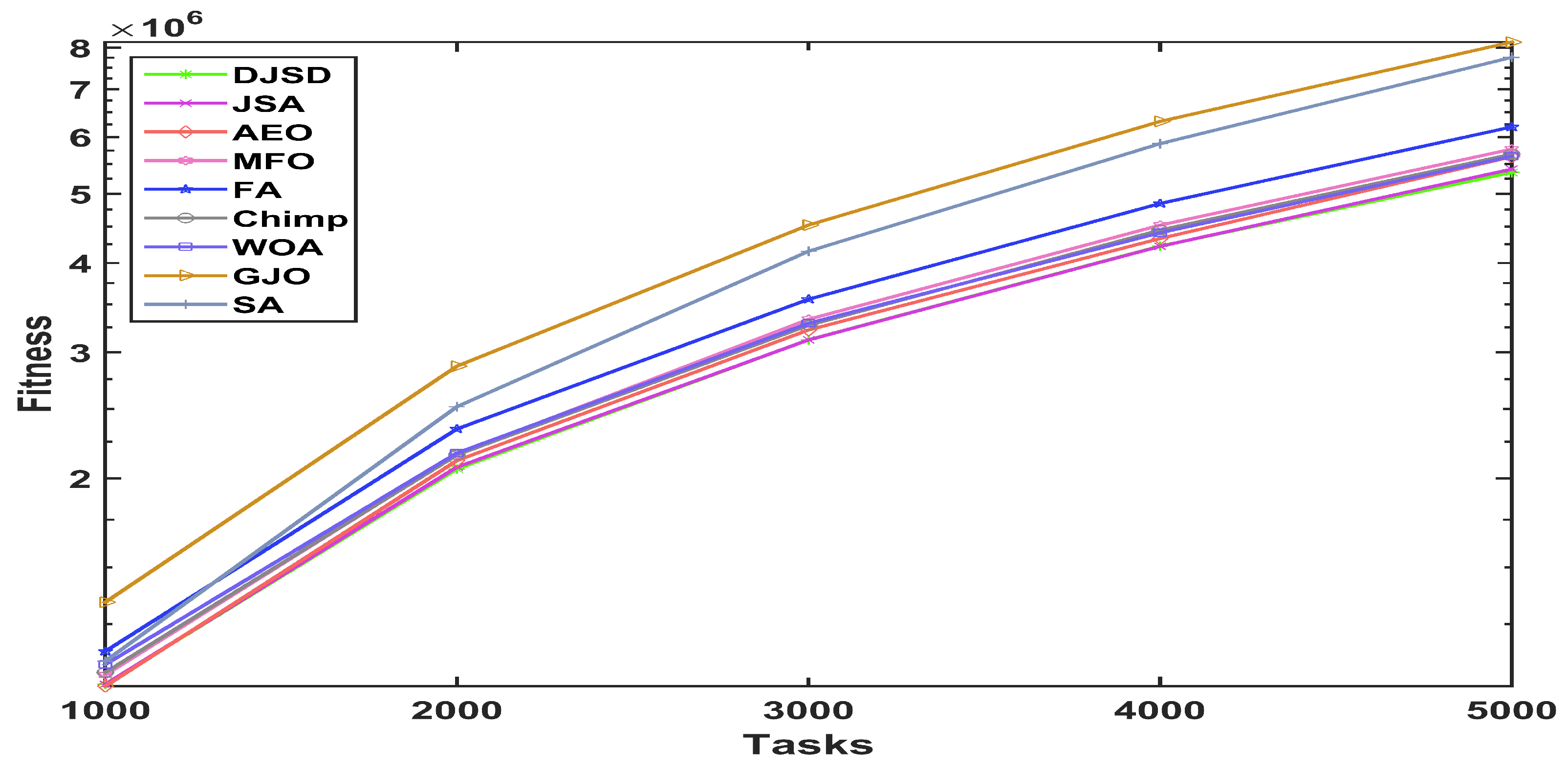
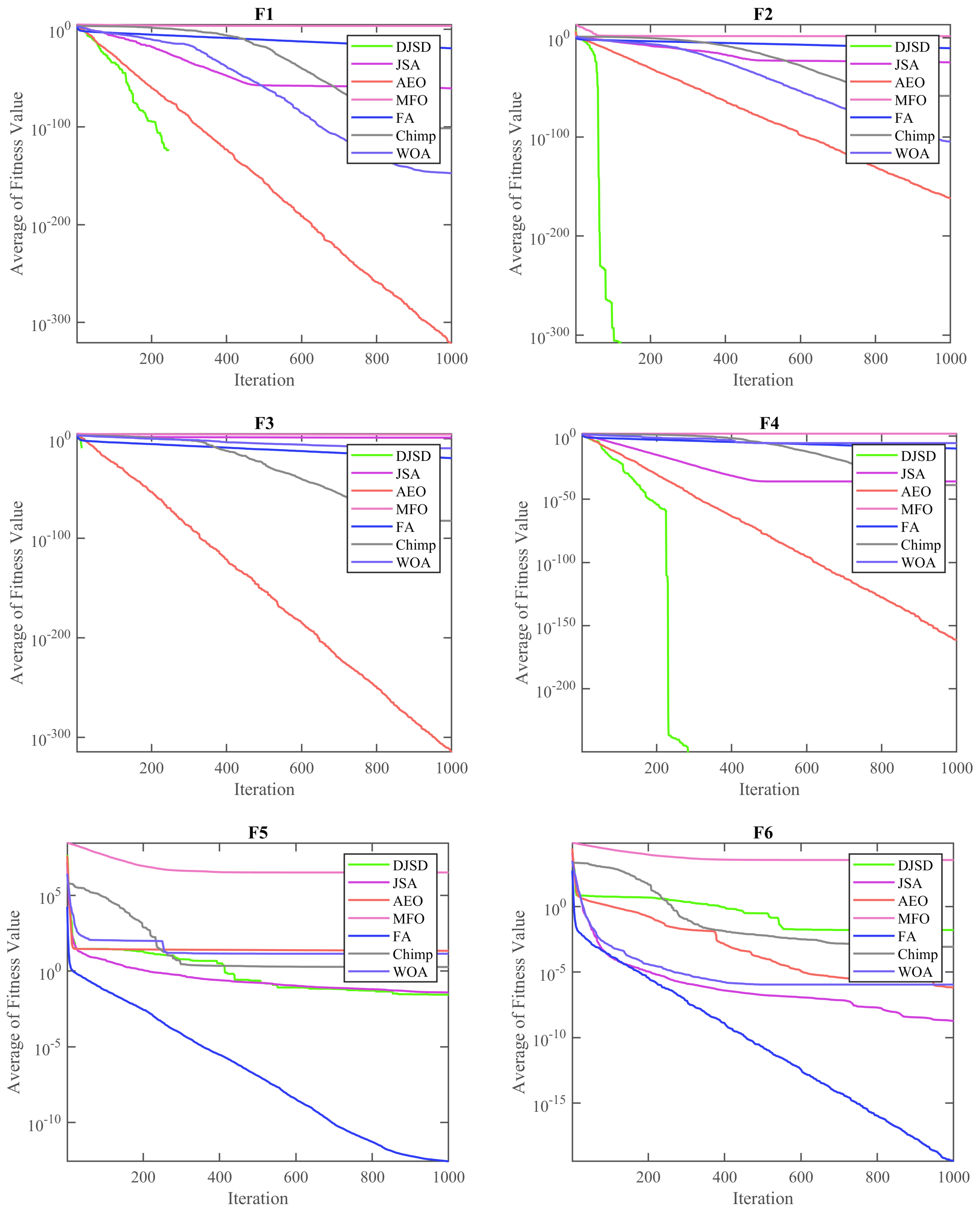
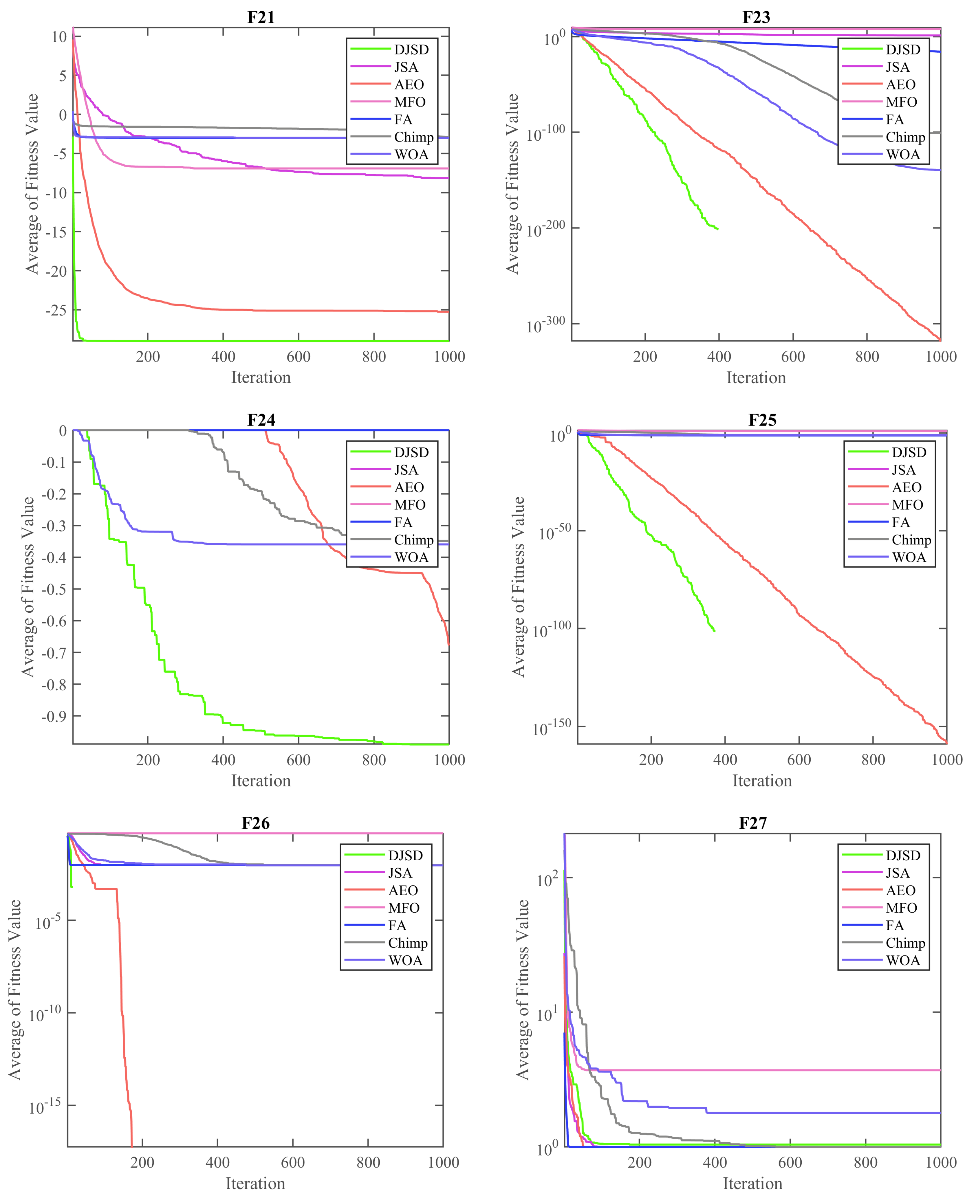
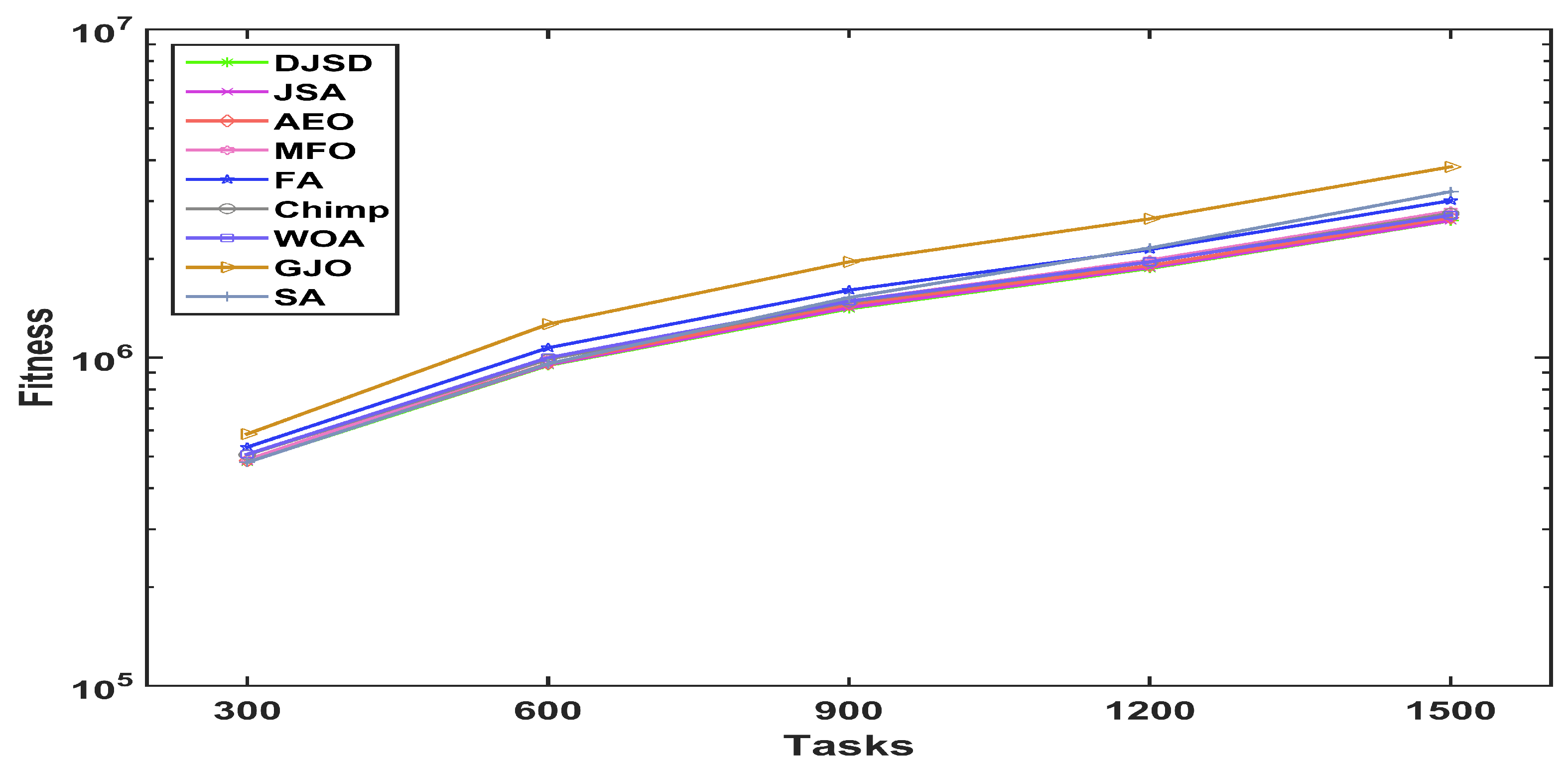
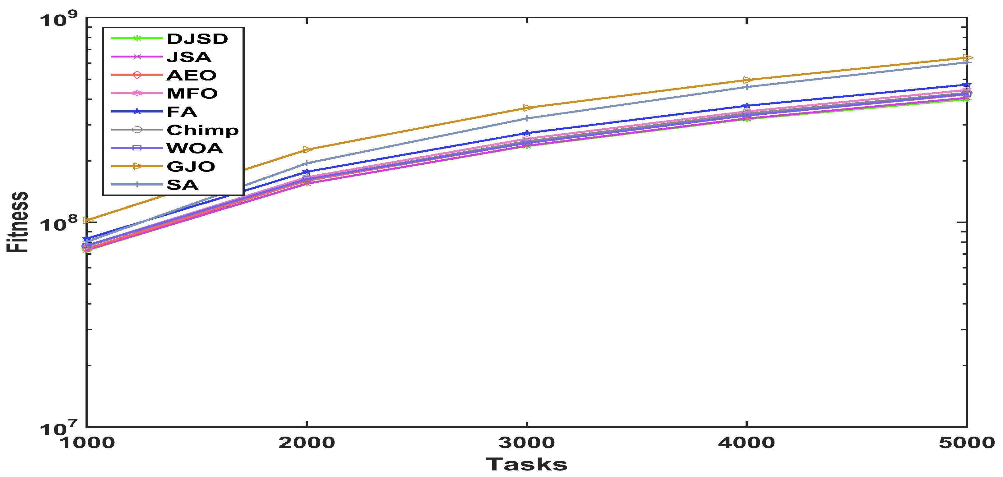
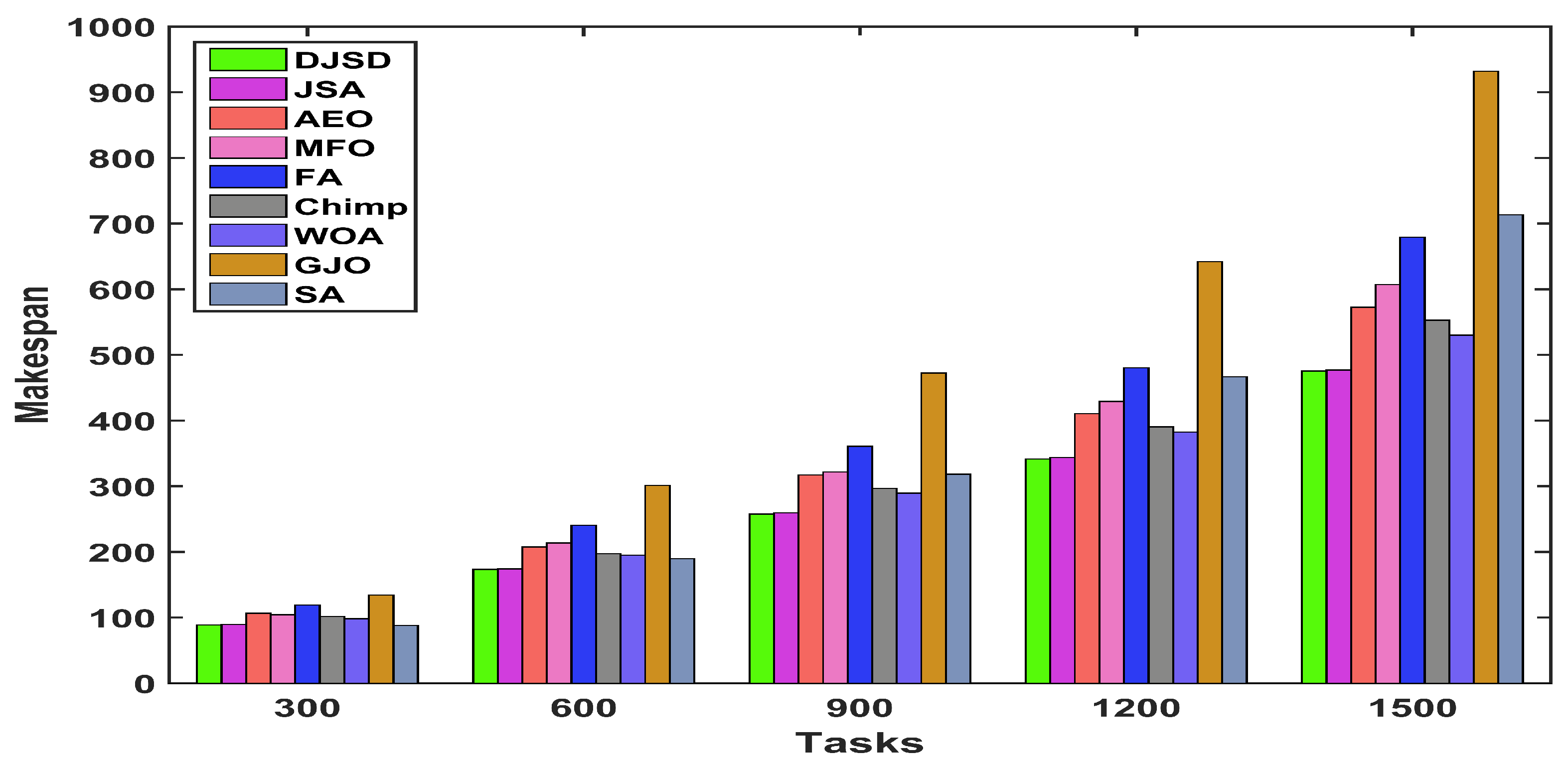
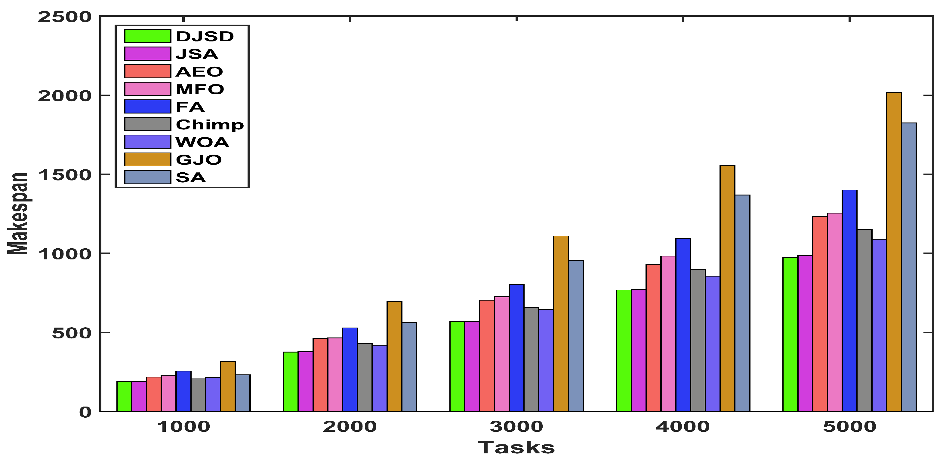
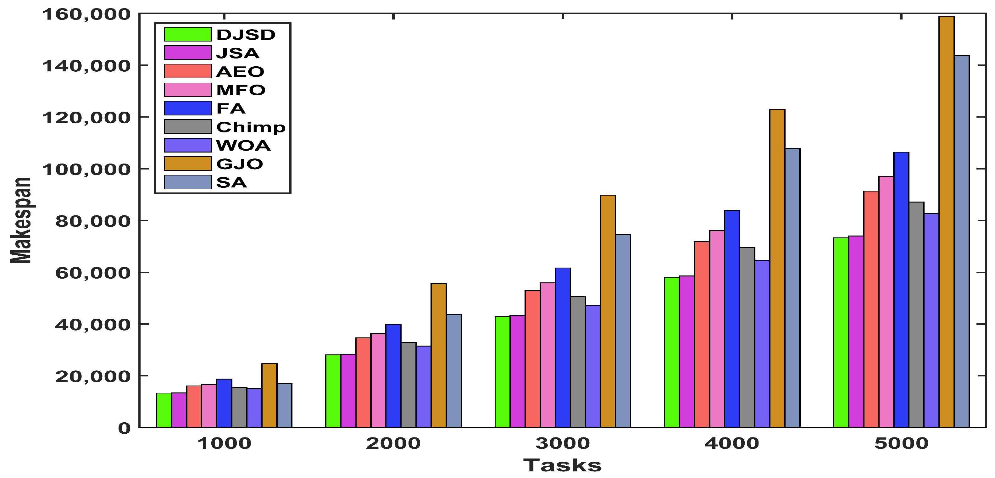
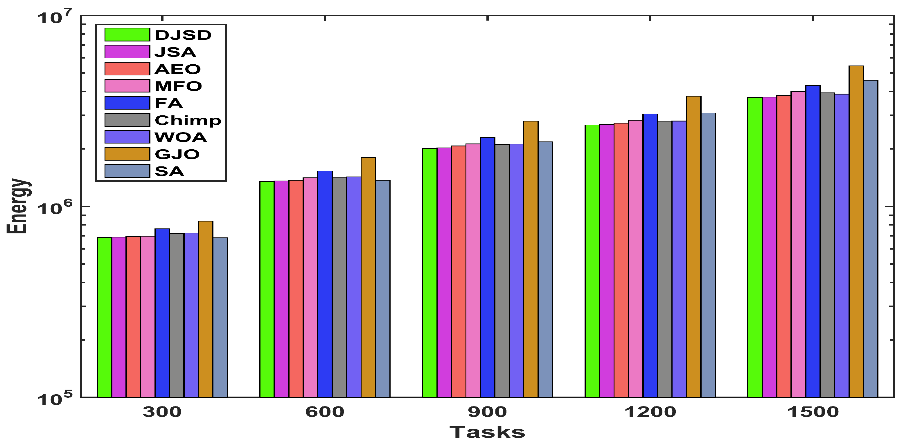
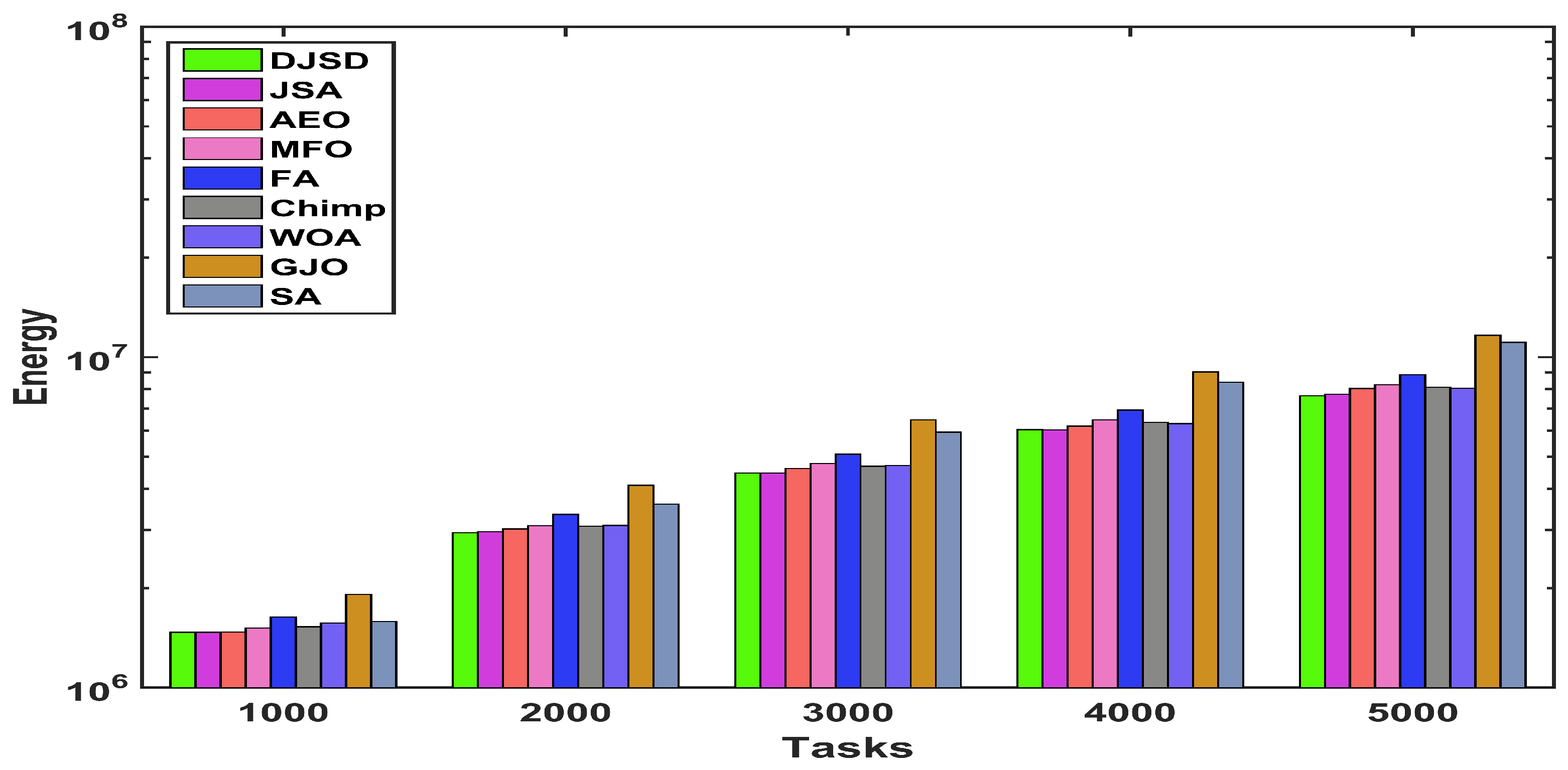
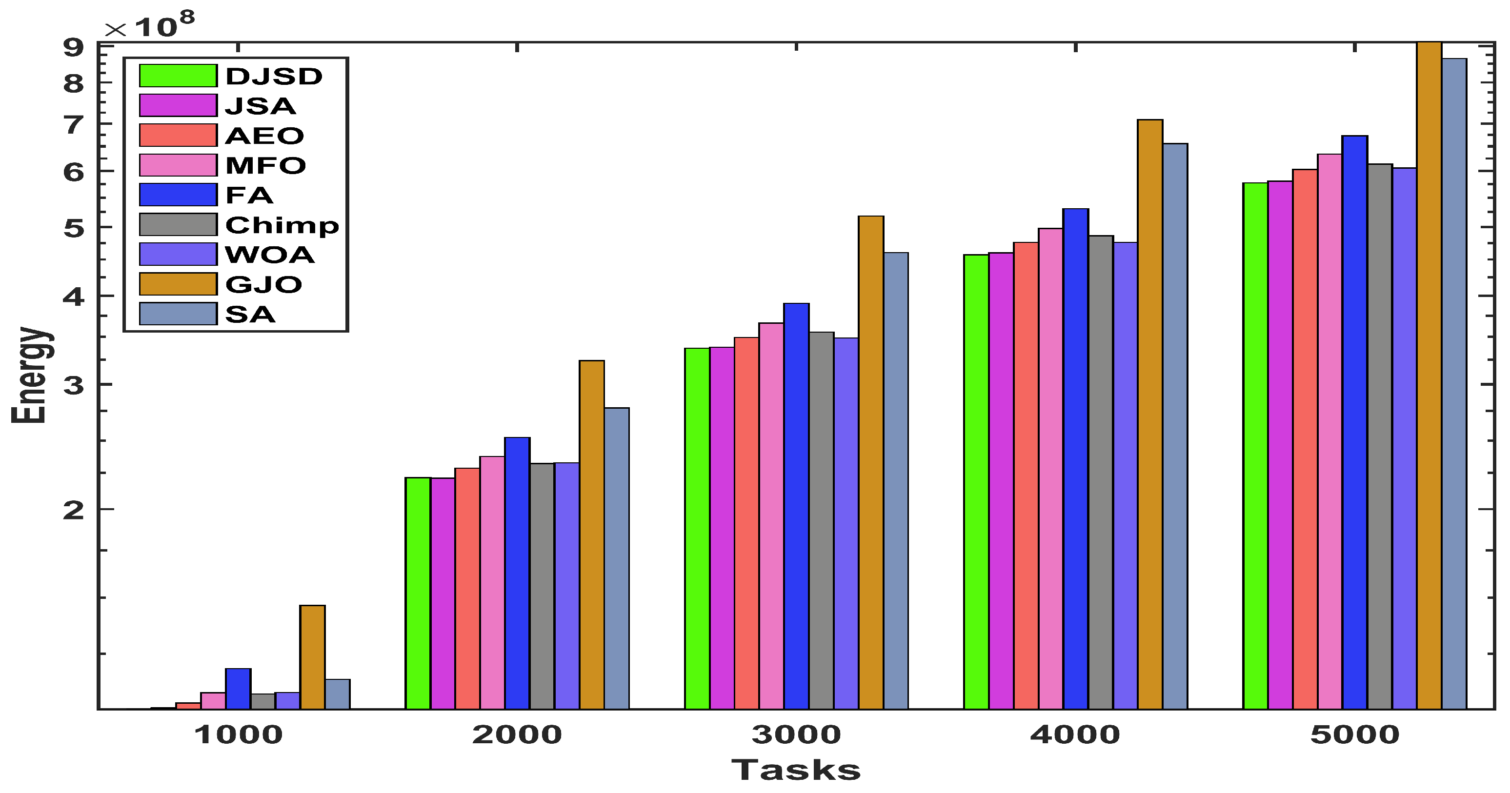
Two experiment series are conducted to validate the performance of the proposed DJSD method. In the first experiment series, thirty classical benchmark functions are used to validate the effectiveness of DJSD compared with other well-known search methods. The findings revealed that the suggested DJSD approach obtained encouraging results, discovered new search regions, and found new best solutions for most test cases. In the second experiment series, a set of tests is conducted to solve cloud computing applications’ task scheduling problems to further prove DJSD’s ability to function in real-world applications. The real-world application results confirmed that the proposed DJSD is competence in dealing with challenging real applications. Moreover, it obtained high performances compared to other similar methods using several standard evaluation measures, including fitness function, makespan, and energy consumption.

The proposed method can be tested further to find potential improvements in future works. Furthermore, it can be combined with other search methods to further improve its searchability in dealing with complicated problems. Different optimization problems can be tested to investigate the performance of the proposed technique, such as text clustering, photovoltaic cell parameters, engineering and industrial optimization problems, forecasting models, feature selection, image segmentation, and multi-objective problems.

References

- Alshinwan, M.; Abualigah, L.; Shehab, M.; Abd Elaziz, M.; Khasawneh, A.M.; Alabool, H.; Al Hamad, H. Dragonfly algorithm: A comprehensive survey of its results, variants, and applications. Multimed. Tools Appl. 2021, 80, 14979–15016. [Google Scholar] [CrossRef]
- Xia, W.; Wu, Z. An effective hybrid optimization approach for multi-objective flexible job-shop scheduling problems. Comput. Ind. Eng. 2005, 48, 409–425. [Google Scholar] [CrossRef]
- He, Q.; Wang, L. An effective co-evolutionary particle swarm optimization for constrained engineering design problems. Eng. Appl. Artif. Intell. 2007, 20, 89–99. [Google Scholar] [CrossRef]
- Karakoyun, M.; Ozkis, A.; Kodaz, H. A new algorithm based on gray wolf optimizer and shuffled frog leaping algorithm to solve the multi-objective optimization problems. Appl. Soft Comput. 2020, 96, 106560. [Google Scholar] [CrossRef]
- Gupta, S.; Deep, K. A memory-based grey wolf optimizer for global optimization tasks. Appl. Soft Comput. 2020, 93, 106367. [Google Scholar] [CrossRef]
- Schuëller, G.I.; Jensen, H.A. Computational methods in optimization considering uncertainties—An overview. Comput. Methods Appl. Mech. Eng. 2008, 198, 2–13. [Google Scholar] [CrossRef]
- Geem, Z.W.; Kim, J.H.; Loganathan, G.V. A new heuristic optimization algorithm: Harmony search. Simulation 2001, 76, 60–68. [Google Scholar] [CrossRef]
- Afshari, H.; Hare, W.; Tesfamariam, S. Constrained multi-objective optimization algorithms: Review and comparison with application in reinforced concrete structures. Appl. Soft Comput. 2019, 83, 105631. [Google Scholar] [CrossRef]
- Gupta, S.; Deep, K.; Mirjalili, S. An efficient equilibrium optimizer with mutation strategy for numerical optimization. Appl. Soft Comput. 2020, 96, 106542. [Google Scholar] [CrossRef]
- Abualigah, L.; Diabat, A.; Mirjalili, S.; Abd Elaziz, M.; Gandomi, A.H. The arithmetic optimization algorithm. Comput. Methods Appl. Mech. Eng. 2021, 376, 113609. [Google Scholar] [CrossRef]
- Bansal, J.C.; Singh, S. A better exploration strategy in Grey Wolf Optimizer. J. Ambient. Intell. Humaniz. Comput. 2021, 12, 1099–1118. [Google Scholar] [CrossRef]
- Abualigah, L.; Yousri, D.; Abd Elaziz, M.; Ewees, A.A.; Al-qaness, M.A.; Gandomi, A.H. Aquila Optimizer: A novel meta-heuristic optimization Algorithm. Comput. Ind. Eng. 2021, 157, 107250. [Google Scholar] [CrossRef]
- Sulaiman, M.H.; Mustaffa, Z.; Saari, M.M.; Daniyal, H. Barnacles mating optimizer: A new bio-inspired algorithm for solving engineering optimization problems. Eng. Appl. Artif. Intell. 2020, 87, 103330. [Google Scholar] [CrossRef]
- Abd Elaziz, M.; Attiya, I. An improved Henry gas solubility optimization algorithm for task scheduling in cloud computing. Artif. Intell. Rev. 2021, 54, 3599–3637. [Google Scholar] [CrossRef]
- Chou, J.S.; Truong, D.N. A novel metaheuristic optimizer inspired by behavior of jellyfish in ocean. Appl. Math. Comput. 2021, 389, 125535. [Google Scholar] [CrossRef]
- Gouda, E.A.; Kotb, M.F.; El-Fergany, A.A. Jellyfish search algorithm for extracting unknown parameters of PEM fuel cell models: Steady-state performance and analysis. Energy 2021, 221, 119836. [Google Scholar] [CrossRef]
- Chou, J.S.; Truong, D.N. Multiobjective optimization inspired by behavior of jellyfish for solving structural design problems. Chaos Solitons Fractals 2020, 135, 109738. [Google Scholar] [CrossRef]
- Manivannan, S.; Selvakumar, S. A Spectrum Defragmentation Algorithm Using Jellyfish Optimization Technique in Elastic Optical Network (EON). Wirel. Pers. Commun. 2021, 1–19. [Google Scholar] [CrossRef]
- Chou, J.S.; Truong, D.N. Multistep energy consumption forecasting by metaheuristic optimization of time-series analysis and machine learning. Int. J. Energy Res. 2021, 45, 4581–4612. [Google Scholar] [CrossRef]
- Dhevanandhini, G.; Yamuna, G. An Efficient Lossless Video Watermarking Extraction Process with Multiple Watermarks Using Artificial Jellyfish Algorithm. Turk. J. Comput. Math. Educ. (TURCOMAT) 2021, 12, 3048–3055. [Google Scholar]
- Ghafil, H.N.; Jármai, K. Dynamic differential annealed optimization: New metaheuristic optimization algorithm for engineering applications. Appl. Soft Comput. 2020, 93, 106392. [Google Scholar] [CrossRef]
- Bertsimas, D.; Tsitsiklis, J. Simulated annealing. Stat. Sci. 1993, 8, 10–15. [Google Scholar] [CrossRef]
- Kirkpatrick, S.; Gelatt, C.D.; Vecchi, M.P. Optimization by simulated annealing. Science 1983, 220, 671–680. [Google Scholar] [CrossRef] [PubMed]
- Ibrahim, R.A.; Abd Elaziz, M.; Lu, S. Chaotic opposition-based grey-wolf optimization algorithm based on differential evolution and disruption operator for global optimization. Expert Syst. Appl. 2018, 108, 1–27. [Google Scholar] [CrossRef]
- Mirjalili, S.; Lewis, A. The whale optimization algorithm. Adv. Eng. Softw. 2016, 95, 51–67. [Google Scholar] [CrossRef]
- Zhao, W.; Wang, L.; Zhang, Z. Artificial ecosystem-based optimization: A novel nature-inspired meta-heuristic algorithm. Neural Comput. Appl. 2020, 32, 9383–9425. [Google Scholar] [CrossRef]
- Khishe, M.; Mosavi, M.R. Chimp optimization algorithm. Expert Syst. Appl. 2020, 149, 113338. [Google Scholar] [CrossRef]
- Yang, X.S. Firefly Algorithms for Multimodal Optimization. In Stochastic Algorithms: Foundations and Applications; Watanabe, O., Zeugmann, T., Eds.; Springer: Berlin/Heidelberg, Germany, 2009; pp. 169–178. [Google Scholar]
- Suganthan, P.N.; Hansen, N.; Liang, J.J.; Deb, K.; Chen, Y.P.; Auger, A.; Tiwari, S. Problem Definitions and Evaluation Criteria for the CEC 2005 Special Session on Real-Parameter Optimization. KanGAL Rep. 2005, 2005005, 2005. [Google Scholar]
- Attiya, I.; Abualigah, L.; Elsadek, D.; Chelloug, S.A.; Abd Elaziz, M. An Intelligent Chimp Optimizer for Scheduling of IoT Application Tasks in Fog Computing. Mathematics 2022, 10, 1100. [Google Scholar] [CrossRef]
- Attiya, I.; Elaziz, M.A.; Abualigah, L.; Nguyen, T.N.; Abd El-Latif, A.A. An Improved Hybrid Swarm Intelligence for Scheduling IoT Application Tasks in the Cloud. IEEE Trans. Ind. Inform. 2022. [Google Scholar] [CrossRef]
- Attiya, I.; Zhang, X.; Yang, X. TCSA: A dynamic job scheduling algorithm for computational grids. In Proceedings of the 2016 First IEEE International Conference on Computer Communication and the Internet (ICCCI), Wuhan, China, 13–15 October 2016; pp. 408–412. [Google Scholar]
- Mishra, S.K.; Puthal, D.; Rodrigues, J.J.P.C.; Sahoo, B.; Dutkiewicz, E. Sustainable Service Allocation Using a Metaheuristic Technique in a Fog Server for Industrial Applications. IEEE Trans. Ind. Inform. 2018, 14, 4497–4506. [Google Scholar] [CrossRef]
- Parallel Workloads Archive. Available online: http://www.cse.huji.ac.il/labs/parallel/workload/logs.html (accessed on 28 April 2021).
- Mirjalili, S. Moth-flame optimization algorithm: A novel nature-inspired heuristic paradigm. Knowl.-Based Syst. 2015, 89, 228–249. [Google Scholar] [CrossRef]
- Chopra, N.; Ansari, M.M. Golden jackal optimization: A novel nature-inspired optimizer for engineering applications. Expert Syst. Appl. 2022, 198, 116924. [Google Scholar] [CrossRef]
Publisher’s Note: MDPI stays neutral with regard to jurisdictional claims in published maps and institutional affiliations. |
© 2022 by the authors. Licensee MDPI, Basel, Switzerland. This article is an open access article distributed under the terms and conditions of the Creative Commons Attribution (CC BY) license (https://creativecommons.org/licenses/by/4.0/).