Double Accelerated Convergence ZNN with Noise-Suppression for Handling Dynamic Matrix Inversion

Abstract

Matrix inversion is commonly encountered in the field of mathematics. Therefore, many methods, including zeroing neural network (ZNN), are proposed to solve matrix inversion. Despite conventional fixed-parameter ZNN (FPZNN), which can successfully address the matrix inversion problem, it may focus on either convergence speed or robustness. So, to surmount this problem, a double accelerated convergence ZNN (DAZNN) with noise-suppression and arbitrary time convergence is proposed to settle the dynamic matrix inversion problem (DMIP). The double accelerated convergence of the DAZNN model is accomplished by specially designing exponential decay variable parameters and an exponential-type sign-bi-power activation function (AF). Additionally, two theory analyses verify the DAZNN model’s arbitrary time convergence and its robustness against additive bounded noise. A matrix inversion example is utilized to illustrate that the DAZNN model has better properties when it is devoted to handling DMIP, relative to conventional FPZNNs employing other six AFs. Lastly, a dynamic positioning example that employs the evolution formula of DAZNN model verifies its availability.

1. Introduction

As a fundamental mathematical issue, matrix inversion plays a crucial role in applied mathematics and engineering fields such as control application [1], quaternion [2], MIMO systems [3,4], and robot kinematics [5,6,7]. Therefore, numerous numerical algorithms have been developed to address this issue. For example, Cholesky decomposition algorithm [8] and Newton iteration algorithm [9] were utilized to solve matrix inversion. However, as the dimensionality of matrix issues increases, the original numerical algorithms are no longer able to handle these complex matrix problems rapidly and effectively [10]. In order to counteract the disadvantages of the above methods, neural networks with the capacity to process problems in parallel were introduced [11]. In addition, neural networks have recently been identified as a hotspot of research, and have been applied to numerous areas, such as medical image denoising [12], hydrogen economy [13], biometric verification [14], quadrotor [15], robots [16], synchronization problem [17], optimal control [18], virus forecasting [19], inflation prediction [20], portfolio optimization, and selection [21,22]. Considering the fact that gradient-based neural networks cannot effectively solve time-varying problems, a zeroing neural network (ZNN), a branch of the recurrent neural network (RNN), was proposed for computing time-variant matrix inversion problem [23].

Nevertheless, as a consequence of the convergence speed limitations, conventional ZNNs with linear activation function (AF) may not be capable of solving large-scale applications online [24]. Consequently, a nonlinear sign-bi-power (SBP) AF was presented in order to shorten the convergence time of ZNN models [25]. ZNN models that use SBPAF for acceleration have been widely reported [26]. However, all the studies mentioned above fail to consider the interference of noise, yet noise is an inherent part of all practical applications [27]. As a result, many researchers proposed a novel class of ZNN models using an integral term to address issues that were affected by noise interference [28,29]. For instance, a modified ZNN model with implicit noise tolerance was proposed by Jin et al. in [30] for the solution of quadratic programming problems. A noise-tolerant ZNN model was investigated to calculate complex matrix inversion with noise [31]. For further research, a unified framework for ZNN with an integral term was investigated, and its superiority to the conventional ZNN model was verified [32].

Regrettably, the vast majority of existing ZNN models containing the aforementioned ZNN models employ fixed convergence parameters, albeit they achieve fast convergence or noise tolerance. As a matter of fact, the convergence parameter generally varies with time in the hardware system [33]. In response to this issue, variable-parameter ZNN/RNN with the characteristics of fast convergence and strong robustness is researched [34,35,36,37]. For example, a variable-gain RNN with fast convergence was proposed for dynamic quadratic programming [34]. Xiao et al. developed a novel varying-parameter ZNN (VPZNN) for handling matrix inversion in [35], which exhibits significantly improved convergence speed when compared with the fixed-parameter ZNN (FPZNN). Further, a varying parameter RNN with an exponential gain time-varying term to resolve matrix inversion was considered [36]. Nevertheless, the variable parameters of the aforesaid VPZNN model tend to be infinite, which is clearly unreasonable in hardware implementations. Thus, we design two exponential decay variable parameters in order to further accelerate the model’s rate. Besides, an exponential-type SBPAF (ETSBPAF) is designed to gain more excellent convergence performance. As such, the double accelerated convergence ZNN (DAZNN) is proposed as a new model for dealing with dynamic matrix inversion problem (DMIP) as it is characterized by noise-suppression and arbitrary time convergence. In addition, the two theory analyses demonstrate the arbitrary time convergence of the DAZNN model as well as its robustness when bounded noises are added. What is more, an illustrative example is employed to assess the validity of the theories, as well as the superiority of DAZNN in comparison with FPZNNs utilizing other AFs (i.e., linear AF, bipolar-sigmoid AF, tunable AF, sign-bi-power AF, predefined time AF, and improved predefined time AF). Lastly, the angle of arrival (AOA) dynamic positioning example that employs the evolution formula of DAZNN model verifies its availability.

Throughout the remainder of this paper, five sections are presented. The problem description and models design are shown in Section 2. In Section 3, we analyze the arbitrary time convergence and robustness of the proposed DAZNN model. An illustrative example is provided in Section 4. Besides, the AOA dynamic positioning simulation with sine noise is conducted in Section 5. Section 6 summarizes the entire work in this paper. The main contributions of this paper are indicated as below.

• As opposed to the ZNN generated by the original error function for the static matrix inversion, this work develops the DAZNN generated by a novel error function to solve dynamic matrix inversion;
• Two new exponential decay variable parameters and a novel exponential-type SBPAF are incorporated into the DAZNN model in order to achieve double accelerated convergence and more stronger noise suppression;
• Two rigorous theoretical analyses are employed in order to demonstrate the arbitrary time convergence of the DAZNN model as well as its robustness under additive bounded noise;
• The illustrative example confirms that the DAZNN model is superior to the fixed-parameter model activated by other six activation functions. Besides, the evolution formula of DAZNN model is applied to the AOA dynamic positioning with sine noise to illustrate the model’s availability further.

2. Problem Formulation and Models Design

In this section, the dynamic matrix inversion problem is presented. Secondly, the design procedures of the fixed-parameter ZNN model and proposed DAZNN model with variable-parameters are introduced.

2.1. Problem Formulation

Consider a dynamic matrix inversion problem (DMIP):

$$\mathcal{A}\left(t\right)\mathcal{X}\left(t\right)=\mathcal{I},$$

(1)

where $\mathcal{A}\left(t\right)\in {\mathbb{R}}^{m\times m}$ is a known non-singular and smooth time-varying coefficient matrix; $\mathcal{X}\left(t\right)\in {\mathbb{R}}^{m\times m}$ is an unknown matrix and $\mathcal{I}\in {\mathbb{R}}^{m\times m}$ denotes the unit matrix.

2.2. Fixed-Parameter ZNN

The general research considers only the ZNN model generated by the original error function (that is, $\mathcal{E}\left(t\right)=\mathcal{A}\left(t\right)\mathcal{X}\left(t\right)-\mathcal{I}$) design without considering the diversity of ZNN models. The diversity of ZNN models can provide more options for hardware implementation. It is easy to see that by designing different error functions, we can obtain different ZNN models based on [38] since the ZNN model is generated by error function and evolution formula [39,40]. Thus, to increase the variety of ZNN model, a novel error function is designed as

$$\mathcal{S}\left(t\right)={\mathcal{A}}^2\left(t\right)\mathcal{X}\left(t\right)-\mathcal{A}\left(t\right).$$

(2)

Then according to the noise tolerance evolution formula [32], we have

$$\frac{d\mathcal{S}\left(t\right)}{dt}=-{\lambda }_1\mathrm{\Omega }\left(\mathcal{S}\left(t\right)\right)-{\lambda }_2\mathrm{\Omega }\left(\mathcal{S}\left(t\right)+{\lambda }_1{\int }_0^t\mathrm{\Omega }\left(\mathcal{S}\left(\tau \right)\right)d\tau \right),$$

(3)

in which ${\lambda }_1,{\lambda }_2>0\in \mathbb{R}$, and $\mathrm{\Omega }(·)$ denotes the odd increasing activation function (AF) array, that is

$$\begin{array}{c}\hfill \begin{array}{c}\hfill \mathrm{\Omega }\left(\mathcal{S}\left(t\right)\right)=\left[\begin{array}{cccc}\omega \left(s_{11}\left(t\right)\right)& \omega \left(s_{12}\left(t\right)\right)& \cdots & \omega \left(s_{1m}\left(t\right)\right)\\ \omega \left(s_{21}\left(t\right)\right)& \omega \left(s_{22}\left(t\right)\right)& \cdots & \omega \left(s_{2m}\left(t\right)\right)\\ ⋮& ⋮& \ddots & ⋮\\ \omega \left(s_{m1}\left(t\right)\right)& \omega \left(s_{m2}\left(t\right)\right)& \cdots & \omega \left(s_{mm}\left(t\right)\right)\end{array}\right],\end{array}\end{array}$$

where $\omega (·)$ is the element of $\mathrm{\Omega }(·)$. In this manner, we can obtain the fix-parameter ZNN (FPZNN) model:

$$\begin{array}{cc}\hfill {\mathcal{A}}^2\left(t\right)\dot{\mathcal{X}}\left(t\right)=& -\left(\mathcal{A}\left(t\right)\dot{\mathcal{A}}\left(t\right)\mathcal{X}\left(t\right)+\dot{\mathcal{A}}\left(t\right)\mathcal{A}\left(t\right)\mathcal{X}\left(t\right)\right)+\dot{\mathcal{A}}\left(t\right)-{\lambda }_1\mathrm{\Omega }\left({\mathcal{A}}^2\left(t\right)\mathcal{X}\left(t\right)-\mathcal{A}\left(t\right)\right)\hfill \\ \hfill & -{\lambda }_2\mathrm{\Omega }\left({\mathcal{A}}^2\left(t\right)\mathcal{X}\left(t\right)-\mathcal{A}\left(t\right)+{\lambda }_1{\int }_0^t\mathrm{\Omega }({\mathcal{A}}^2\left(\tau \right)\mathcal{X}\left(\tau \right)-\mathcal{A}\left(\tau \right))d\tau \right).\hfill \end{array}$$

(4)

Listed below are some commonly used AF that we use to compare to the novel AF.

(1)

Linear AF (LAF) [41]:

$$\omega \left(z\right)=z.$$

(5)

(2)

Bipolar-sigmoid AF (BSAF) [25]:

$$\omega \left(z\right)=\frac{1+exp(-r)}{1-exp(-r)}·\frac{1+exp(-rz)}{1-exp(-rz)},$$

(6)

where $r>2$.

(3)

Tunable AF (TAF) [42]:

$$\omega \left(z\right)=k_1{\left|z\right|}^q\mathrm{sign}\left(z\right)+{\varpi }_{1}z,$$

(7)

where $0<q<1$, $k_1,{\varpi }_1>0$.

(4)

Sign-bi-power AF (SBPAF) [25]:

$$\omega \left(z\right)=\left({0.5\left|z\right|}^q+0.5{\left|z\right|}^{1/q}\right)\mathrm{sign}\left(z\right),$$

(8)

where $\mathrm{sign}(·)$ is defined as

$$\mathrm{sign}\left(z\right)=\left\{\begin{array}{cc}1,\hfill & \mathrm{if}z>0,\hfill \\ 0,\hfill & \mathrm{if}z=0,\hfill \\ -1,\hfill & \mathrm{if}z<0.\hfill \end{array}\right.$$

(5)

Predefined time AF (PTAF) [43]:

$$\omega \left(z\right)=\left(k_1{\left|z\right|}^q+k_2{\left|z\right|}^p\right)\mathrm{sign}\left(z\right)+k_{3}z+k_4\mathrm{sign}\left(z\right),$$

(9)

where $p>1$, $k_2>0$ and $k_3,k_4\ge 0$.

(6)

Improved predefined time AF (IPTAF) [10]:

$$\begin{array}{c}\hfill \omega \left(z\right)=\left\{\begin{array}{cc}{k}_1{\left|z\right|}^q\mathrm{sign}\left(z\right)+k_{5}z,\hfill & \mathrm{if}\left|z\right|\le 1,\hfill \\ k_2{\left|z\right|}^p\mathrm{sign}\left(z\right)+k_{5}z,\hfill & \mathrm{if}\left|z\right|>1,\hfill \end{array}\right.\end{array}$$

(10)

where $k_1,k_2$ are the same as defined above and $k_5>0$.

2.3. DAZNN Model

While the FPZNN is a powerful tool for handling DMIP, we are aware that it is inferior to the variable-parameter ZNN from [10,34,35] due to its fix-parameter nature. Therefore, a double accelerated convergence ZNN (DAZNN) model is proposed to solve DMIP.

Firstly, according to the novel variable parameters, the variable-parameter evolution formula can be depicted as [10,32]:

$$\frac{d\mathcal{S}\left(t\right)}{dt}=-{\varrho }_1\left(t\right){\mathrm{\Omega }}_1\left(\mathcal{S}\left(t\right)\right)-{\varrho }_2\left(t\right){\mathrm{\Omega }}_2\left(\mathcal{S}\left(t\right)+{\int }_0^t{\varrho }_1\left(\tau \right){\mathrm{\Omega }}_1\left(\mathcal{S}\left(\tau \right)\right)d\tau \right),$$

(11)

where ${\mathrm{\Omega }}_1(·)$ and ${\mathrm{\Omega }}_2(·)$ represent AF arrays. Besides, ${\omega }_1(·)$ and ${\omega }_2(·)$ are the elements in ${\mathrm{\Omega }}_1(·)$ and ${\mathrm{\Omega }}_2(·)$. And ${\omega }_1(·)$ and ${\omega }_2(·)$ denote exponential-type SBPAF (ETSBPAF) as

$${\omega }_1\left(z\right)={\omega }_2\left(z\right)=exp({\mu }_1\left|z\right|+{\mu }_2)\left({0.5\left|z\right|}^q+0.5{\left|z\right|}^{1/q}\right)\mathrm{sign}\left(z\right),$$

(12)

with ${\mu }_1,{\mu }_2>0\in \mathbb{R}$ and ${\varrho }_1\left(t\right)$ and ${\varrho }_2\left(t\right)$ can be defined by

$$\begin{array}{c}\hfill {\varrho }_1\left(t\right)={\lambda }_{1}exp\left({\phi }_1\mathrm{arccot}\left(t\right)\right),{\varrho }_2\left(t\right)={\lambda }_{2}exp\left({\phi }_2\mathrm{arccot}\left(t\right)\right),\end{array}$$

(13)

with ${\lambda }_1,{\lambda }_2,{\phi }_1,{\phi }_2>0\in \mathbb{R}$. Therefore, the DAZNN model is written as

$$\begin{array}{cc}\hfill {\mathcal{A}}^2\left(t\right)\dot{\mathcal{X}}\left(t\right)=& -\left(\mathcal{A}\left(t\right)\dot{\mathcal{A}}\left(t\right)\mathcal{X}\left(t\right)+\dot{\mathcal{A}}\left(t\right)\mathcal{A}\left(t\right)\mathcal{X}\left(t\right)\right)+\dot{\mathcal{A}}\left(t\right)-{\varrho }_1\left(t\right){\mathrm{\Omega }}_1\left({\mathcal{A}}^2\left(t\right)\mathcal{X}\left(t\right)-\mathcal{A}\left(t\right)\right)\hfill \\ \hfill & -{\varrho }_2\left(t\right){\mathrm{\Omega }}_2\left({\mathcal{A}}^2\left(t\right)\mathcal{X}\left(t\right)-\mathcal{A}\left(t\right)+{\int }_0^t{\varrho }_1\left(t\right){\mathrm{\Omega }}_1({\mathcal{A}}^2\left(\tau \right)\mathcal{X}\left(\tau \right)-\mathcal{A}\left(\tau \right))d\tau \right).\hfill \end{array}$$

(14)

In this part, by deriving the noise tolerance evolution design formula, a specific DAZNN model is proposed for solving the DMIP (1).

3. Theoretical Analysis

In this section, the arbitrary time convergence and robustness performance of the DAZNN model (14) are theoretically analyzed. The corresponding results are given as below.

3.1. Arbitrary Time Convergence

Theorem 1.

Given an invertible matrix $\mathcal{A}\left(t\right)$, and starting from any initial value $\mathcal{X}\left(0\right)$, DAZNN model (14) with ETSBPAF can converge to zero in the arbitrary time

$$\begin{array}{c}\hfill t_{\mathrm{c}}\le \left\{\begin{array}{cc}\frac{q({\theta }_1+{\theta }_2)}{{\theta }_1{\theta }_{2}exp\left({\mu }_1\right)(1-q)}+\frac{{\theta }_1+{\theta }_2}{{\theta }_1{\theta }_2(1-q)},\hfill & if\mathcal{H}\left(0\right)>1and\mathcal{L}\left(t_{c1}\right)>1,\hfill \\ \frac{q}{{\theta }_{2}exp\left({\mu }_1\right)(1-q)}+\frac{{\theta }_1+{\theta }_2}{{\theta }_1{\theta }_2(1-q)},\hfill & if\mathcal{H}\left(0\right)>1and\mathcal{L}\left(t_{c1}\right)\le 1,\hfill \\ \frac{q}{{\theta }_{1}exp\left({\mu }_1\right)(1-q)}+\frac{{\theta }_1+{\theta }_2}{{\theta }_1{\theta }_2(1-q)},\hfill & if\mathcal{H}\left(0\right)\le 1and\mathcal{L}\left(t_{c1}\right)>1,\hfill \\ \frac{{\theta }_1+{\theta }_2}{{\theta }_1{\theta }_2(1-q)},\hfill & if\mathcal{H}\left(0\right)\le 1and\mathcal{L}\left(t_{c1}\right)\le 1,\hfill \end{array}\right.\end{array}$$

in which ${\theta }_1=0.5{\lambda }_{1}exp\left({\mu }_2\right)$, ${\theta }_2=0.5{\lambda }_{2}exp\left({\mu }_2\right)$.

Proof of Theorem 1.

The DAZNN model (14) can convert to evolution formula (11), let $s_{ij}\left(t\right)$ denote the elements of $\mathcal{S}\left(t\right)$, and the subsystem of DAZNN model (14) can be directly analyzed as

$${\dot{s}}_{ij}\left(t\right)=-{\varrho }_1\left(t\right){\omega }_1\left(s_{ij}\left(t\right)\right)-{\varrho }_2\left(t\right){\omega }_2\left(s_{ij}\left(t\right)+{\int }_0^t{\varrho }_1\left(\tau \right){\omega }_1\left(s_{ij}\left(\tau \right)\right)d\tau \right),$$

(15)

with $i,j=1,2,\dots ,m$. For the sake of better carrying on convergence analysis, an intermediate variable is introduced as

$$u_{ij}\left(t\right)=s_{ij}\left(t\right)+{\int }_0^t{\varrho }_1\left(\tau \right){\omega }_1\left(s_{ij}\left(\tau \right)\right)d\tau ,$$

(16)

which implies that

$$\begin{array}{c}\hfill {\dot{u}}_{ij}\left(t\right)={\dot{s}}_{ij}\left(t\right)+{\varrho }_1\left(t\right){\omega }_1\left(s_{ij}\left(t\right)\right)=-{\varrho }_2\left(t\right){\omega }_2\left(u_{ij}\left(t\right)\right).\end{array}$$

(17)

For this dynamic system, a Lyapunov function (LF) is constructed as $\mathcal{H}\left(t\right)=|u_{ij}\left(t\right)|$. Note that $\mathcal{H}\left(t\right)$ is a positive definite function and radially unbounded, then

$$\begin{array}{cc}\hfill \dot{\mathcal{H}}\left(t\right)& ={\dot{u}}_{ij}\left(t\right)\mathrm{sign}\left(u_{ij}\left(t\right)\right)\hfill \\ \hfill & =-{\varrho }_2\left(t\right){\omega }_2\left(u_{ij}\left(t\right)\right)\mathrm{sign}\left(u_{ij}\left(t\right)\right)\hfill \\ \hfill & =-0.5{\lambda }_{2}exp\left({\phi }_2\mathrm{arccot}\left(t\right)\right)exp({\mu }_1|u_{ij}\left(t\right)|+{\mu }_2)\left(|u_{ij}{|}^q\left(t\right)+{\left|u_{ij}\right|}^{1/q}\left(t\right)\right)\hfill \\ \hfill & =-0.5{\lambda }_{2}exp\left({\mu }_2\right)exp({\mu }_1|u_{ij}\left(t\right)\left|\right)\left(|u_{ij}{|}^q\left(t\right)+{\left|u_{ij}\right|}^{1/q}\left(t\right)\right)\hfill \\ \hfill & =-{\theta }_{2}exp\left({\mu }_1\mathcal{H}\left(t\right)\right)\left({\mathcal{H}}^q\left(t\right)+{\mathcal{H}}^{1/q}\left(t\right)\right),\hfill \end{array}$$

(18)

in which ${\theta }_2=0.5{\lambda }_{2}exp\left({\mu }_2\right)$. It is evident that $\dot{\mathcal{H}}\left(t\right)$ is negative definite, so the zero solution of $\mathcal{H}\left(t\right)$ is globally asymptotically stable. That is, $\dot{\mathcal{H}}\left(t\right)$ can decay to zero within time $t_{c1}=t_1+t_2$. Without losing generality, we consider $\mathcal{H}\left(0\right)=|u_{ij}\left(0\right)|>1$ and $\mathcal{H}\left(0\right)=|u_{ij}\left(0\right)|\le 1$.

Case one: $\mathcal{H}\left(0\right)=|u_{ij}\left(0\right)|>1$. First step, $\mathcal{H}\left(0\right)>1$ will decay to $\mathcal{H}\left(t_1\right)=1$ after time $t_1$; the second step, $\mathcal{H}\left(t_1\right)=1$ will decay to $\mathcal{H}(t_1+t_2)=0$ after time $t_1+t_2$.

Step (a): $\mathcal{H}\left(0\right)>1\to \mathcal{H}\left(t_1\right)=1$. Equation (18) can be written as

$$\begin{array}{cc}\hfill \dot{\mathcal{H}}\left(t\right)& =-{\theta }_{2}exp\left({\mu }_1\mathcal{H}\left(t\right)\right)\left({\mathcal{H}}^q\left(t\right)+{\mathcal{H}}^{1/q}\left(t\right)\right)\hfill \\ \hfill & \le -{\theta }_{2}exp\left({\mu }_1\right){\mathcal{H}}^{1/q}\left(t\right).\hfill \end{array}$$

(19)

Inequality (19) can be expressed as

$$\begin{array}{cc}\hfill \mathcal{H}{\left(t\right)}^{-1/q}\mathrm{d}\mathcal{H}& \le -{\theta }_{2}exp\left({\mu }_1\right)\mathrm{d}t.\hfill \end{array}$$

(20)

Integrate both sides of the inequality (20) from 0 to $t_1$:

$$\begin{array}{cc}\hfill {\int }_{\mathcal{H}\left(0\right)}^{\mathcal{H}\left(t_1\right)}\mathcal{H}{\left(t\right)}^{-1/q}\mathrm{d}\mathcal{H}& \le {\int }_0^{t_1}-{\theta }_{2}exp\left({\mu }_1\right)\mathrm{d}t.\hfill \end{array}$$

(21)

By virtue of $\mathcal{H}\left(t_1\right)=1$,

$$\begin{array}{cc}\hfill t_1& \le \frac{q\left(1-{\mathcal{H}}^{1-1/q}\left(0\right)\right)}{{\theta }_{2}exp\left({\mu }_1\right)(1-q)}\le \frac{q}{{\theta }_{2}exp\left({\mu }_1\right)(1-q)}.\hfill \end{array}$$

(22)

Step (b): $|u_{ij}\left(t_1\right)|=1\to |u_{ij}(t_1+t_2)|=0$. Equation (18) is written as

$$\begin{array}{cc}\hfill \dot{\mathcal{H}}\left(t\right)& =-{\theta }_{2}exp\left({\mu }_1\mathcal{H}\left(t\right)\right)\left({\mathcal{H}}^q\left(t\right)+{\mathcal{H}}^{1/q}\left(t\right)\right)\hfill \\ \hfill & \le -{\theta }_2{\mathcal{H}}^q\left(t\right).\hfill \end{array}$$

(23)

Integrate both sides of the inequality (23) from $t_1$ to $t_1+t_2$:

$$\begin{array}{cc}\hfill {\int }_{\mathcal{H}\left(t_1\right)}^{\mathcal{H}(t_1+t_2)}\mathcal{H}{\left(t\right)}^{-q}\mathrm{d}\mathcal{H}& \le {\int }_{t_1}^{t_1+t_2}-{\theta }_2\mathrm{d}t.\hfill \end{array}$$

(24)

We can derive

$$\begin{array}{cc}\hfill t_2& \le \frac{1}{{\theta }_2(1-q)}.\hfill \end{array}$$

(25)

Then, we can get convergence time $t_{\mathrm{c}1}$ of the first process in case one:

$$\begin{array}{c}\hfill t_{c1}=t_1+t_2\le \frac{q}{{\theta }_{2}exp\left({\mu }_1\right)(1-q)}+\frac{1}{{\theta }_2(1-q)}.\end{array}$$

(26)

At this point, $\mathcal{H}\left(t\right)$ can converge to zero in case-one.

Case two: $\mathcal{H}\left(0\right)=|u_{ij}\left(0\right)|\le 1$. Then, $\mathcal{H}\left(0\right)\le 1$ will decay to $\mathcal{H}\left(t_{21}\right)=0$ after time $t_{21}$. We have: $|u_{ij}\left(0\right)|\le 1\to |u_{ij}\left(t_{21}\right)|=0$. Equation (18) is written as

$$\begin{array}{cc}\hfill \dot{\mathcal{H}}\left(t\right)& =-{\theta }_{2}exp\left({\mu }_1\mathcal{H}\left(t\right)\right)\left({\mathcal{H}}^q\left(t\right)+{\mathcal{H}}^{1/q}\left(t\right)\right)\hfill \\ \hfill & \le -{\theta }_2{\mathcal{H}}^q\left(t\right).\hfill \end{array}$$

(27)

Integrate both sides of the inequality (27) from 0 to $t_{21}$:

$$\begin{array}{cc}\hfill {\int }_{\mathcal{H}\left(0\right)}^{\mathcal{H}\left(t_{21}\right)}\mathcal{H}{\left(t\right)}^{-q}\mathrm{d}\mathcal{H}& \le {\int }_0^{t_{21}}-{\theta }_2\mathrm{d}t.\hfill \end{array}$$

(28)

We can derive

$$\begin{array}{c}\hfill t_{21}\le \frac{{\mathcal{H}}^{1-q}\left(0\right)}{{\theta }_2(1-q)}\le \frac{1}{{\theta }_2(1-q)}.\end{array}$$

(29)

Then, we can get convergence time $t_{\mathrm{c}1}$ of the first process in case two:

$$\begin{array}{c}\hfill t_{c1}=t_{21}\le \frac{1}{{\theta }_2(1-q)}.\end{array}$$

(30)

Thus, the convergence time $t_{c1}$ of the first process can be calculated:

$$\begin{array}{c}\hfill t_{c1}\le \left\{\begin{array}{cc}\frac{q}{{\theta }_{2}exp\left({\mu }_1\right)(1-q)}+\frac{1}{{\theta }_2(1-q)},\hfill & \mathrm{if}\mathcal{H}\left(0\right)=|u_{ij}\left(0\right)|>1,\hfill \\ \frac{1}{{\theta }_2(1-q)},\hfill & \mathrm{if}\mathcal{H}\left(0\right)=|u_{ij}\left(0\right)|\le 1.\hfill \end{array}\right.\end{array}$$

So, the subsystem (15) can be expressed as

$${\dot{s}}_{ij}\left(t\right)=-{\varrho }_1\left(t\right){\omega }_1\left(s_{ij}\left(t\right)\right).$$

(31)

Devise a new LF $\mathcal{L}\left(t\right)$ as

$$\mathcal{L}\left(t\right)=|s_{ij}\left(t\right)|.$$

(32)

Further, the derivative of $\mathcal{L}\left(t\right)$ can be obtained:

$$\begin{array}{cc}\hfill \dot{\mathcal{L}}\left(t\right)& ={\dot{s}}_{ij}\left(t\right)\mathrm{sign}\left(s_{ij}\left(t\right)\right)\hfill \\ \hfill & =-{\varrho }_1\left(t\right){\omega }_1\left(s_{ij}\left(t\right)\right)\mathrm{sign}\left(s_{ij}\left(t\right)\right)\hfill \\ \hfill & =-0.5{\lambda }_{1}exp\left({\phi }_1\mathrm{arccot}\left(t\right)\right)exp({\mu }_1|s_{ij}\left(t\right)|+{\mu }_2)\left(|s_{ij}{|}^q\left(t\right)+{\left|s_{ij}\right|}^{1/q}\left(t\right)\right)\hfill \\ \hfill & =-0.5{\lambda }_{1}exp\left({\mu }_2\right)exp({\mu }_1|s_{ij}\left(t\right)\left|\right)\left(|s_{ij}{|}^q\left(t\right)+{\left|s_{ij}\right|}^{1/q}\left(t\right)\right)\hfill \\ \hfill & =-{\theta }_{1}exp\left({\mu }_1\mathcal{L}\left(t\right)\right)\left({\mathcal{L}}^q\left(t\right)+{\mathcal{L}}^{1/q}\left(t\right)\right),\hfill \end{array}$$

(33)

where ${\theta }_1=0.5{\lambda }_{1}exp\left({\mu }_2\right)$. Evidently, the zero solution of $\mathcal{L}\left(t\right)$ is globally asymptotically stable. Analogously, consider $\mathcal{L}\left(t_{c1}\right)=\left|s_{ij}\left(t_{c1}\right)\right|>1$ and $\mathcal{L}\left(t_{c1}\right)=\left|s_{ij}\left(t_{c1}\right)\right|\le 1$.

Case one: $\mathcal{L}\left(t_{c1}\right)=\left|s_{ij}\left(t_{c1}\right)\right|>1$. $\mathcal{L}\left(t_{c1}\right)>1$ decreased to $\mathcal{L}(t_{c1}+t_3)=1$ in the first step; $\mathcal{L}(t_{c1}+t_3)=1$ decreased to $\mathcal{L}(t_{c1}+t_3+t_4)=0$ in the second step. In a similar way, $t_3$ and $t_4$ can be calculated:

$$\begin{array}{c}\hfill t_3\le \frac{q}{{\theta }_{1}exp\left({\mu }_1\right)(1-q)},t_4\le \frac{1}{{\theta }_1(1-q)}.\end{array}$$

(34)

Case two: $\mathcal{L}\left(t_{c1}\right)=\left|s_{ij}\left(t_{c1}\right)\right|\le 1$. Then, $\mathcal{H}\left(0\right)\le 1$ will decay to $\mathcal{H}\left(t_{22}\right)=0$ after time $t_{22}$. Similarly, we have:

$$\begin{array}{c}\hfill t_{22}\le \frac{1}{{\theta }_1(1-q)}.\end{array}$$

(35)

Furthermore, convergence time $t_{c2}$ of the second process is calculated as

$$\begin{array}{c}\hfill t_{c2}\le \left\{\begin{array}{cc}\frac{q}{{\theta }_{1}exp\left({\mu }_1\right)(1-q)}+\frac{1}{{\theta }_1(1-q)},\hfill & \mathrm{if}\mathcal{L}\left(t_{c1}\right)=\left|s_{ij}\left(t_{c1}\right)\right|>1,\hfill \\ \frac{1}{{\theta }_1(1-q)},\hfill & \mathrm{if}\mathcal{L}\left(t_{c1}\right)=\left|s_{ij}\left(t_{c1}\right)\right|\le 1.\hfill \end{array}\right.\end{array}$$

Then, we can get the total convergence time $t_{\mathrm{c}}$:

$$\begin{array}{c}\hfill t_{\mathrm{c}}\le \left\{\begin{array}{cc}\frac{q({\theta }_1+{\theta }_2)}{{\theta }_1{\theta }_{2}exp\left({\mu }_1\right)(1-q)}+\frac{{\theta }_1+{\theta }_2}{{\theta }_1{\theta }_2(1-q)},\hfill & \mathrm{if}\mathcal{H}\left(0\right)>1\mathrm{and}\mathcal{L}\left(t_{c1}\right)>1,\hfill \\ \frac{q}{{\theta }_{2}exp\left({\mu }_1\right)(1-q)}+\frac{{\theta }_1+{\theta }_2}{{\theta }_1{\theta }_2(1-q)},\hfill & \mathrm{if}\mathcal{H}\left(0\right)>1\mathrm{and}\mathcal{L}\left(t_{c1}\right)\le 1,\hfill \\ \frac{q}{{\theta }_{1}exp\left({\mu }_1\right)(1-q)}+\frac{{\theta }_1+{\theta }_2}{{\theta }_1{\theta }_2(1-q)},\hfill & \mathrm{if}\mathcal{H}\left(0\right)\le 1\mathrm{and}\mathcal{L}\left(t_{c1}\right)>1,\hfill \\ \frac{{\theta }_1+{\theta }_2}{{\theta }_1{\theta }_2(1-q)},\hfill & \mathrm{if}\mathcal{H}\left(0\right)\le 1\mathrm{and}\mathcal{L}\left(t_{c1}\right)\le 1.\hfill \end{array}\right.\end{array}$$

(36)

Note that the upper bound of our calculated time $t_{\mathrm{c}}$ is independent of initial value $\mathcal{X}\left(0\right)$. Thus the proof is now completed. □

3.2. Robustness

Theorem 2.

Given a nonsingular matrix $A\left(t\right)$, and starting from any initial value $X\left(0\right)$, the DAZNN model (14) with additive bounded noise $\xi \left(t\right)$ ($|{\xi }_{ij}\left(t\right)|\le a$ and a is constant) can converge to zero or be bounded by

$$\begin{array}{c}\hfill \underset{t\to \infty }{lim}{∥\mathcal{S}\left(t\right)∥}_F\le \frac{2am}{{\lambda }_{1}exp\left({\mu }_2\right)},\end{array}$$

where m represents dimension of coefficient matrix.

Proof of Theorem 2.

According to the subsystem of DAZNN model (14) and additive noise $\xi \left(t\right)$, it can be obtained:

$${\dot{s}}_{ij}\left(t\right)=-{\varrho }_1\left(t\right){\omega }_1\left(s_{ij}\left(t\right)\right)-{\varrho }_2\left(t\right){\omega }_2\left(s_{ij}\left(t\right)+{\int }_0^t{\varrho }_1\left(\tau \right){\omega }_1\left(s_{ij}\left(\tau \right)\right)d\tau \right)+{\xi }_{ij}\left(t\right).$$

(37)

Then, we separate into two parts for analysis, the first part is set a intermediate variable, the same as Equation (16), and the time derivative of the intermediate variable is ${\dot{u}}_{ij}\left(t\right)={\dot{s}}_{ij}\left(t\right)+{\varrho }_1\left(t\right){\omega }_1\left(s_{ij}\left(t\right)\right)$, then substituting $u_{ij}\left(t\right)$ and ${\dot{u}}_{ij}\left(t\right)$ into Equation (37), the first system can be acquired:

$${\dot{u}}_{ij}\left(t\right)=-{\varrho }_2\left(t\right){\omega }_2\left(u_{ij}\left(t\right)\right)+{\xi }_{ij}\left(t\right).$$

(38)

Introduce the Lyapunov function to analyze the first system (38):

$$\mathcal{G}\left(t\right)=\frac{1}{2}{u}_{ij}^2\left(t\right).$$

(39)

Then

$$\begin{array}{c}\hfill \dot{\mathcal{G}}\left(t\right)=u_{ij}\left(t\right){\dot{u}}_{ij}\left(t\right)=u_{ij}\left(t\right)(-{\varrho }_2\left(t\right){\omega }_2\left(u_{ij}\left(t\right)\right)+{\xi }_{ij}\left(t\right)).\end{array}$$

(40)

(a) If $\dot{\mathcal{G}}\left(t\right)>0$, $|u_{ij}\left(t\right)|$ will gradually increase, and $u_{ij}\left(t\right){\xi }_{ij}\left(t\right)>0$. In this case, $\dot{\mathcal{G}}\left(t\right)>0$, that is

$$\begin{array}{c}\hfill u_{ij}\left(t\right)(-{\varrho }_2\left(t\right){\omega }_2\left(u_{ij}\left(t\right)\right)+{\xi }_{ij}\left(t\right))>0.\end{array}$$

Hence, we get

$$\begin{array}{c}\hfill |{\xi }_{ij}\left(t\right)|>|{\varrho }_2\left(t\right){\omega }_2\left(u_{ij}\left(t\right)\right)|.\end{array}$$

By virtue of the noise ${\xi }_{ij}\left(t\right)$ is bounded, it is easy to know that $|-{\varrho }_2\left(t\right){\omega }_2\left(u_{ij}\left(t\right)\right)+{\xi }_{ij}\left(t\right)|$ will decrease as $|u_{ij}\left(t\right)|$ increases. Besides, $|u_{ij}\left(t\right)|$ will stop increasing until $-{\varrho }_2\left(t\right){\omega }_2\left(u_{ij}\left(t\right)\right)+{\xi }_{ij}\left(t\right)=0$. It shows that the change will eventually enter a stable state, that is, the final $\dot{\mathcal{G}}\left(t\right)=0$ holds true. It is not hard to get:

$$\begin{array}{c}\hfill {\dot{s}}_{ij}\left(t\right)=-{\varrho }_1\left(t\right){\omega }_1\left(s_{ij}\left(t\right)\right).\end{array}$$

(41)

Besides, $s_{ij}\left(t\right)=0$ is globally asymptotically stable from Theorem 1, namely

$$\begin{array}{c}\hfill \underset{t\to \infty }{lim}{∥\mathcal{S}\left(t\right)∥}_{\mathrm{F}}=0.\end{array}$$

(b) If $\dot{\mathcal{G}}\left(t\right)<0$, then $|u_{ij}\left(t\right)|$ will gradually decrease to zero. Then, the degraded form of the subsystem (33) is expressed as

$${\dot{s}}_{ij}\left(t\right)=-{\varrho }_1\left(t\right){\omega }_1\left(s_{ij}\left(t\right)\right)+{\xi }_{ij}\left(t\right).$$

(42)

(b1) ${\dot{s}}_{ij}\left(t\right)<0$. At this time, $s_{ij}\left(t\right)=0$ is globally asymptotically stable. That is

$$\begin{array}{c}\hfill \underset{t\to \infty }{lim}{∥\mathcal{S}\left(t\right)∥}_{\mathrm{F}}=0.\end{array}$$

(b2) ${\dot{s}}_{ij}\left(t\right)>0$. This situation is similar to the above situation (a). In the end, we can get $-{\varrho }_1\left(t\right){\omega }_1\left(s_{ij}\left(t\right)\right)+{\xi }_{ij}\left(t\right)=0$. Obviously, when $t\to \infty$, $|s_{ij}\left(t\right)|$ is bounded by

$$\begin{array}{c}\hfill 0\le |s_{ij}\left(t\right)|\le \left|{\omega }_1^{-1}\left(\frac{{\xi }_{ij}\left(t\right)}{{\varrho }_1\left(t\right)}\right)\right|,\end{array}$$

where ${\omega }_1^{-1}(·)$ is the inverse function of ${\omega }_1(·)$. Due to $|{\omega }_1\left(z\right)|\ge |0.5exp\left({\mu }_2\right)z|$ such that $|{\omega }_1^{-1}\left(z\right)|\le |2z/exp\left({\mu }_2\right)|$ keeps correct. And the bound of $|s_{ij}\left(t\right)|$ can be written as

$$\begin{array}{c}\hfill 0\le |s_{ij}\left(t\right)|\le \left|\frac{2{\xi }_{ij}\left(t\right)}{exp\left({\mu }_2\right){\varrho }_1\left(t\right)}\right|=\left|\frac{2{\xi }_{ij}\left(t\right)}{{\lambda }_{1}exp\left({\mu }_2\right)exp\left({\phi }_1\mathrm{arccot}\left(t\right)\right)}\right|.\end{array}$$

(43)

Then, by virtue of $|{\xi }_{ij}\left(t\right)|\le a$,

$$\begin{array}{cc}\hfill \underset{t\to \infty }{lim}{∥\mathcal{S}\left(t\right)∥}_{\mathrm{F}}& =\underset{t\to \infty }{lim}\sqrt{\sum _{i=1}^m\sum _{j=1}^m{\left|s_{ij}\left(t\right)\right|}^2}\hfill \\ \hfill & \le \underset{t\to \infty }{lim}\sqrt{\sum _{i=1}^m\sum _{j=1}^m{\left(\frac{2{\xi }_{ij}\left(t\right)}{{\lambda }_{1}exp\left({\mu }_2\right)exp\left({\phi }_1\mathrm{arccot}\left(t\right)\right)}\right)}^2}\hfill \\ \hfill & \le \frac{2am}{{\lambda }_{1}exp\left({\mu }_2\right)}.\hfill \end{array}$$

(c) If $\dot{\mathcal{G}}\left(t\right)=0$, we can know that $u_{ij}\left(t\right)=0$ or $-{\varrho }_2\left(t\right){\omega }_2\left(u_{ij}\left(t\right)\right)+{\xi }_{ij}\left(t\right)=0$. This case is similar as case (a) or case (b), so $\underset{t\to \infty }{lim}{∥\mathcal{S}\left(t\right)∥}_{\mathrm{F}}$ can converge to zero or be bounded.

In the end, it is concluded that in the unknown bounded noise environment, the error of model (14) can converge to zero or be bounded. □

4. Illustrative Verification

In this section, the FPZNN models with different AFs and DAZNN model (14) are applied to online solving dynamic matrix inversion problem, and the comparison results are shown as below.

Consider this time-varying matrix:

$$\mathcal{A}\left(t\right)=\left[\begin{array}{cc}sin\left(3t\right)& cos\left(3t\right)\\ -cos\left(3t\right)& sin\left(3t\right)\end{array}\right],$$

and ${\mathcal{A}}^{*}\left(t\right)$ denotes the theoretical solution of the Equation (1), in other words, ${\mathcal{A}}^{*}\left(t\right)={\mathcal{A}}^{-1}\left(t\right)$. Besides, in this simulation, some public parameters are: $k_1=k_2=0.5$, $q=1/p=0.2$; the parameter of AF (6) is set as $r=3$; the parameter of AF (7) is set as ${\varpi }_1=10$; the parameters of AF (9) are set as $k_3=0.2$, $k_4=0$; the parameter of AF (10) is set as $k_5=0.2$; the parameters of AF (12) are set as ${\mu }_1=1$, ${\mu }_2=0.5$; variable parameters (13) are set as ${\phi }_1={\phi }_2=0.3$; and $\mathcal{X}\left(0\right)\in {[-1,1]}^{2\times 2}$.

4.1. Discussion of Convergence

As seen in Figure 1, the state solutions (i.e., ${\mathcal{X}}_{11}\left(t\right)$, ${\mathcal{X}}_{12}\left(t\right)$, ${\mathcal{X}}_{21}\left(t\right)$, ${\mathcal{X}}_{22}\left(t\right)$) and theoretical solutions (i.e., ${\mathcal{X}}_{11}^{*}\left(t\right)$, ${\mathcal{X}}_{12}^{*}\left(t\right)$, ${\mathcal{X}}_{21}^{*}\left(t\right)$, ${\mathcal{X}}_{22}^{*}\left(t\right)$) are put together to compare. According to the results, in addition to the FPZNN models activated by AFs (5)–(7), other FPZNN models with different AFs and DAZNN model (14) can converge without noise. Moreover, it is clear that FPZNN with AF (12) has the fastest convergence speed.

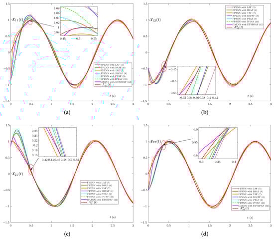
Figure 1. Trajectories of the solutions $\mathcal{X}\left(t\right)$ of different models, of which the red line denotes the theoretical solution ${\mathcal{X}}_{ij}^{*}\left(t\right)$ with no noise. (a) Theoretical solution ${\mathcal{X}}_{11}^{*}\left(t\right)$ and state solutions ${\mathcal{X}}_{11}\left(t\right)$. (b) Theoretical solution ${\mathcal{X}}_{12}^{*}\left(t\right)$ and state solutions ${\mathcal{X}}_{12}\left(t\right)$. (c) Theoretical solution ${\mathcal{X}}_{21}^{*}\left(t\right)$ and state solutions ${\mathcal{X}}_{21}\left(t\right)$. (d) Theoretical solution ${\mathcal{X}}_{22}^{*}\left(t\right)$ and state solutions ${\mathcal{X}}_{22}\left(t\right)$.

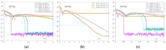
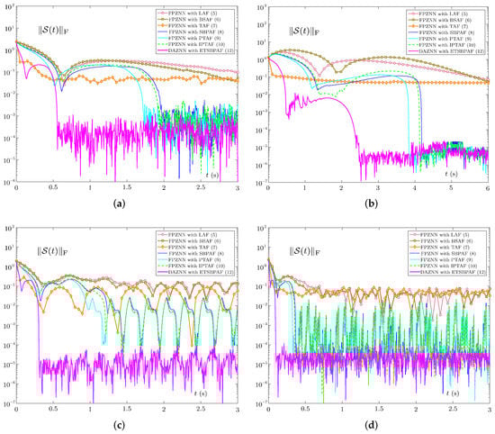
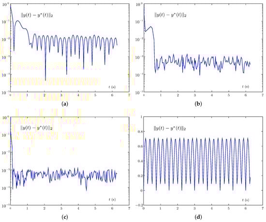
Secondly, Figure 2 comprehensively reveals the errors ${\parallel \mathcal{S}\left(t\right)\parallel }_{\mathrm{F}}$ of these ZNN models in the absence of noise. As illustrated in Figure 2a,b, it is evident that with no noise and ${\lambda }_1={\lambda }_2=1.5$, the errors of both of these models can drop to zero. However, the error accuracy of model (4) activated by AF (7) can only reach $5\times {10}^{-2}$, while other models can reach a higher error accuracy. Aside from model (4) activated by AF (7), the convergence rate of these models rank as follows: model (14) activated by AF (12), model (4) activated by AF (9), model (4) activated by AF (10), model (4) activated by AF (8), model (4) activated by AF (6), model (4) activated by AF (5). In addition, Figure 2c suggests that the errors of the convergence time corresponding to these ZNN models is reduced a lot with ${\lambda }_1={\lambda }_2=15$, which also verifies Theorem 1.

Figure 2. Dynamic characteristics of the ${\parallel \mathcal{S}\left(t\right)\parallel }_{\mathrm{F}}$ by FPZNN model (4) and DAZNN model (14) with no noise and different ${\lambda }_1={\lambda }_2$. (a) With ${\lambda }_1={\lambda }_2=1.5$. (b) With ${\lambda }_1={\lambda }_2=1.5$. (c) With ${\lambda }_1={\lambda }_2=15$.

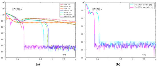
Finally, we control the variables in order to further demonstrate the specific impact of the two improvements (i.e., variable parameters (13) and AF (12)) in the new model, as shown in Figure 3. Specifically, Figure 3a illustrates the model errors ${\parallel \mathcal{S}\left(t\right)\parallel }_{\mathrm{F}}$ for FPZNN with various AFs. Figure 3b discloses the errors of the FPZNN model (4) activated by AF (12) and DAZNN model (14). It is not difficult to discover that the FPZNN model activated by AF (12) has the best convergence performance in the seven AFs used from Figure 3a. This means that AF (12) has the best acceleration effect on the model. Moreover, for the condition of employing AF (12), the DAZNN model (14) performs better than the FPZNN model (4). Therefore, we can draw a conclusion that both AF (12) and variable parameters (13) have a gain effect on the convergence rate of the model.

Figure 3. Dynamic characteristics of the ${\parallel \mathcal{S}\left(t\right)\parallel }_{\mathrm{F}}$ by FPZNN model (4) and DAZNN model (14). (a) FPZNN model (4) with various AFs. (b) FPZNN model (4) with AF (12) and DAZNN model (14).

4.2. Discussion of Robustness

In fact, in the circuit implementation of RNN, additive noise is inevitable. Additionally, the additive noise can result in the failure of the original algorithm or other undesirable effects. Therefore, the robustness of a model is a key indicator of a model’s performance.

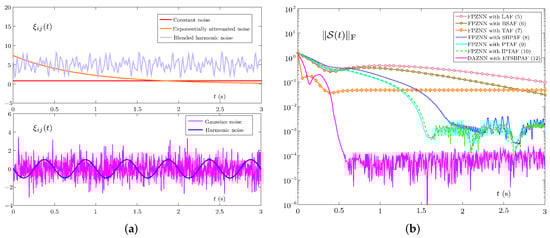
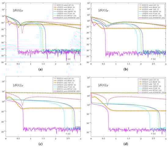
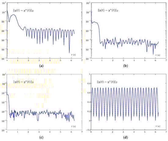
First, five kinds of noise dynamic characteristics are shown in Figure 4a. Specifically, there are five types of noise: constant noise ${\xi }_{ij}\left(t\right)=0.8$, Gaussian noise ${\xi }_{ij}$ with zero mean and one standard deviation, exponentially attenuated noise ${\xi }_{ij}\left(t\right)=exp(-1.2t+2)$, harmonic noise ${\xi }_{ij}\left(t\right)=sin(4\pi t+\pi )$ and blended harmonic noise ${\xi }_{ij}\left(t\right)=sin(10\pi t-\pi )+sin(30\pi t+3)+sin(34\pi t-4)+sin(50\pi t+7)$. Figure 4b reveals the errors ${\parallel \mathcal{S}\left(t\right)\parallel }_{\mathrm{F}}$ of these ZNN models under noise ${\xi }_{ij}\left(t\right)=0.8$. The error accuracy and convergence speed of all models display a certain degree of decline, even when they are subject to disturbances of constant noise ${\xi }_{ij}\left(t\right)=0.8$. Compared with other models, the DAZNN model (14) is the least affected and still has the highest convergence speed and accuracy.

Figure 4. Profile of different noises, and dynamic characteristics of the ${\parallel \mathcal{S}\left(t\right)\parallel }_{\mathrm{F}}$ by FPZNN model (4) and DAZNN model (14) with noise. (a) Profile of different noises. (b) With constant noise ${\xi }_{ij}\left(t\right)=0.8$.

As a means of further verifying the robustness of the DAZNN model (14), we tested its dynamic characteristic of errors under four other bounded noises in Figure 5. Observing Figure 5a,b, it is found that in the case of Gaussian noise, the convergence speed of these models is not affected much, but the error accuracy is significantly reduced. On the contrary, in an exponential attenuated noise environment, the error accuracy of these models is basically unchanged, but the convergence time is significantly increased. In Figure 5c, in the case of harmonic noise ${\xi }_{ij}\left(t\right)=sin(4\pi t+\pi )$ and ${\lambda }_1={\lambda }_2=2.5$, the DAZNN model (14) is not greatly affected, but the accuracy of other models is greatly reduced. The result in Figure 5d is similar, in the case of blended harmonic noise ${\xi }_{ij}\left(t\right)=sin(10\pi t-\pi )+sin(30\pi t+3)+sin(34\pi t-4)+sin(50\pi t+7)$ and ${\lambda }_1={\lambda }_2=8$, the DAZNN model (14) is not markedly affected. In general, the error accuracy and convergence speed of all models decrease to varying degrees, but relatively speaking, the DAZNN model (14) is the least affected. These results provide support for our theoretical analysis that the DAZNN model (14) can accomplish robustness to bounded noise.

Figure 5. Dynamic characteristics of the ${\parallel \mathcal{S}\left(t\right)\parallel }_{\mathrm{F}}$ by FPZNN model (4) and DAZNN model (14) with disparate bounded noises and different ${\lambda }_1,{\lambda }_2$. (a) Gaussian noise and ${\lambda }_1={\lambda }_2=1.5$. (b) Exponentially attenuated noise ${\xi }_{ij}\left(t\right)=exp(-1.2t+2)$ and ${\lambda }_1={\lambda }_2=1.5$. (c) Harmonic noise ${\xi }_{ij}\left(t\right)=sin(4\pi t+\pi )$ and ${\lambda }_1={\lambda }_2=2.5$. (d) Blended harmonic noise ${\xi }_{ij}\left(t\right)=sin(10\pi t-\pi )+sin(30\pi t+3)+sin(34\pi t-4)+sin(50\pi t+7)$ and ${\lambda }_1={\lambda }_2=8$.

4.3. Sensitivity of Initial Values

The convergence performance of many ZNN models will be affected by the initial value, but related studies have rarely been addressed. Therefore, the sensitivity of the model to the initial value is worth discussing.

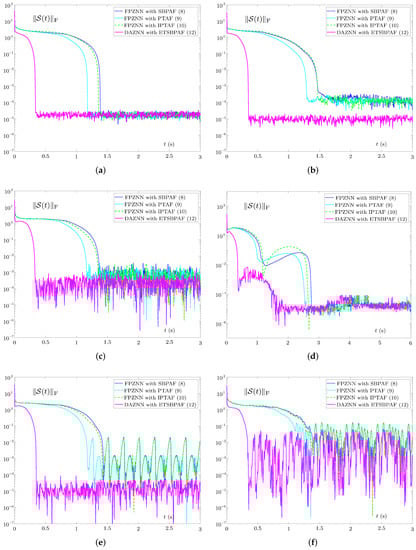
To demonstrate the impact of random starting values on these models’ errors, an experiment is conducted. Four random initial values belonging to different intervals are tested, as shown in Figure 6. The error accuracy of four models including DAZNN model (14) and FPZNN models with AFs (8)–(10) can reach ${10}^{-5}$ under various $\mathcal{X}\left(0\right)$. The convergence times of the four models above under different initial values are as follows: DAZNN model (14) takes about 0.48 s, 0.58 s, 0.71 s, and 0.71 s; FPZNN model with AF (9) is about 1.45 s, 1.86 s, 2.35 s, and 2.35 s; FPZNN model with AF (10) is about 1.49 s, 2.05 s, 2.72 s, and 2.72 s; FPZNN model with AF (8) is about 1.60 s, 2.15 s, 2.78 s, and 2.78 s. Relatively speaking, although the convergence time of DAZNN model (14) also relies on $\mathcal{X}\left(0\right)$, the dependence on the initial value is smaller. Besides, it is not difficult to know that the convergence time of the above four models has an upper bound that has nothing to do with the initial value $\mathcal{X}\left(0\right)$. It is worth noting that these models have a characteristic, that is, the activation functions used all have ${\left|z\right|}^q\mathrm{sign}\left(z\right)$ term, which shows to a certain extent that power term is a necessary term for the predefined convergent activation function.

Figure 6. Dynamic characteristics of the ${\parallel \mathcal{S}\left(t\right)\parallel }_{\mathrm{F}}$ by FPZNN model (4) and DAZNN model (14) in different initial values $\mathcal{X}\left(0\right)$. (a) $\mathcal{X}\left(0\right)\in {[-0.7,0.7]}^{2\times 2}$. (b) $\mathcal{X}\left(0\right)\in {[-4,4]}^{2\times 2}$. (c) $\mathcal{X}\left(0\right)\in {[-70,70]}^{2\times 2}$. (d) $\mathcal{X}\left(0\right)\in {[-400,400]}^{2\times 2}$.

In this part, this example verifies the convergence and robustness performance of the DAZNN model (14) using multiple model comparisons when solving dynamic matrix inversion problem (1).

4.4. High Dimensional Example Verification

Considering another $4\times 4$ time-variant Toeplitz matrix:

$$\mathcal{A}\left(t\right)=\left[\begin{array}{cccc}3+sin\left(0.5t\right)& cos\left(0.5t\right)& cos\left(0.5t\right)/2& cos\left(0.5t\right)/3\\ cos\left(0.5t\right)& 3+sin\left(0.5t\right)& cos\left(0.5t\right)& cos\left(0.5t\right)/2\\ cos\left(0.5t\right)/2& cos\left(0.5t\right)& 3+sin\left(0.5t\right)& cos\left(0.5t\right)\\ cos\left(0.5t\right)/3& cos\left(0.5t\right)/2& cos\left(0.5t\right)& 3+sin\left(0.5t\right)\end{array}\right].$$

Note that the performance of the first three models (including PZNN with LAF (5), FPZNN with BSAF (6), and FPZNN with TAF (7)) is not good, so we just consider other models for comparison in this example. Besides, the conditions for this example are set to be the same as before, except that ${\lambda }_1={\lambda }_2=3$.

Figure 7 shows the dynamic trajectories of error norms ${\parallel \mathcal{S}\left(t\right)\parallel }_{\mathrm{F}}$ of these ZNN models under noise or bounded noise. At this time, the DAZNN model still shows excellent model performance. It is known from Figure 7a that all models can converge without noise. From Figure 7b,e, when the noise is constant noise ${\xi }_{ij}\left(t\right)=0.8$ or harmonic noise ${\xi }_{ij}\left(t\right)=sin(4\pi t+\pi )$, the accuracy of DAZNN model (14) is significantly higher than the other three models. Moreover, as shown in Figure 7c,d,f, under the interference of other noises, although the accuracy of DAZNN model (14) is similar to the other three models, its convergence speed is still much faster. In general, Section 4.4 fully demonstrates that the proposed DAZNN model has the best performance among these four models in a higher dimensional example.

Figure 7. Dynamic characteristics of the ${\parallel \mathcal{S}\left(t\right)\parallel }_{\mathrm{F}}$ by FPZNN model (4) and DAZNN model (14) with no noise or disparate bounded noises. (a) No noise. (b) Constant noise ${\xi }_{ij}\left(t\right)=0.8$. (c) Gaussian noise. (d) Exponentially attenuated noise ${\xi }_{ij}\left(t\right)=exp(-1.2t+2)$. (e) Harmonic noise ${\xi }_{ij}\left(t\right)=sin(4\pi t+\pi )$. (f) Blended harmonic noise ${\xi }_{ij}\left(t\right)=sin(10\pi t-\pi )+sin(30\pi t+3)+sin(34\pi t-4)+sin(50\pi t+7)$.

5. Application to Dynamic Positioning Algorithm

This section first briefly describes the dynamic positioning problem based on the angle of arrival (AOA). Secondly, to validate the efficacy of the DAZNN model, design formula (11) and design formula (3) are applied to the AOA positioning algorithm.

5.1. Problem Description

The angle of arrival (AOA) positioning method’s main principle is to calculate the angle of arrival between the target and the sensor node [44]. Taking the sensor node as the starting point and passing through the target node will form a ray. The point where the two rays intersect is the position of the target node.

Suppose the coordinates of n fixed sensor nodes are $(w_l,z_l)$, represented by the matrix B, where $l=1,2,\dots ,n$; the incident angle of sensor nodes is ${\beta }_l\left(t\right)$, represented by the vector $\beta \left(t\right)$; consider the two-dimensional situation, the target node position at time t uses the unknown vector $y\left(t\right)={[w\left(t\right),z\left(t\right)]}^{\mathrm{T}}$. The specific mathematical expression is as follows

$$\begin{array}{c}\hfill B=\left[\begin{array}{ccccc}{w}_1& w_2& w_3& \dots & w_n\\ z_1& z_2& z_3& \dots & z_n\end{array}\right]\in {\mathbb{R}}^{2\times n},\beta \left(t\right)={\left[\begin{array}{cccc}{\beta }_1\left(t\right)& {\beta }_2\left(t\right)& \cdots & {\beta }_n\left(t\right)\end{array}\right]}^{\mathrm{T}}\in {\mathbb{R}}^n.\end{array}$$

Hence, the incident angle ${\beta }_l\left(t\right)$ satisfies

$$tan\left({\beta }_l\left(t\right)\right)=\frac{z\left(t\right)-z_l}{w\left(t\right)-w_l}.$$

The following equation can be further derived:

$$\begin{array}{c}\hfill \left[\begin{array}{c}{z}_1-w_{1}tan\left({\beta }_1\left(t\right)\right)\\ z_2-w_{2}tan\left({\beta }_2\left(t\right)\right)\\ ⋮\\ z_n-w_{n}tan\left({\beta }_n\left(t\right)\right)\end{array}\right]=\left[\begin{array}{cc}-tan\left({\beta }_1\left(t\right)\right)& 1\\ -tan\left({\beta }_2\left(t\right)\right)& 1\\ ⋮& ⋮\\ -tan\left({\beta }_n\left(t\right)\right)& 1\end{array}\right]\left[\begin{array}{c}w\left(t\right)\\ z\left(t\right)\end{array}\right].\end{array}$$

(44)

Equation (44) can be converted to the following form:

$$Q\left(t\right)=P\left(t\right)y\left(t\right),$$

(45)

where $P\left(t\right)\in {\mathbb{R}}^{n\times 2}$ represents the smooth dynamic matrix with full column rank, $Q\left(t\right)\in {\mathbb{R}}^{n\times 1}$ denotes a smooth dynamic vector.

5.2. Model Application

First define an error:

$$e\left(t\right)=P\left(t\right)y\left(t\right)-Q\left(t\right).$$

(46)

Multiplying both sides of Equation (46) by $P^{\mathrm{T}}\left(t\right)$, we can get the new error:

$$ϵ\left(t\right)=P^{\mathrm{T}}\left(t\right)P\left(t\right)y\left(t\right)-P^{\mathrm{T}}\left(t\right)Q\left(t\right)\in {\mathbb{R}}^{2\times 1}.$$

(47)

The derivative of Equation (47) can be obtained:

$$\begin{array}{c}\hfill \dot{ϵ}\left(t\right)={\dot{P}}^{\mathrm{T}}\left(t\right)P\left(t\right)y\left(t\right)+P^{\mathrm{T}}\left(t\right)\dot{P}\left(t\right)y\left(t\right)+P^{\mathrm{T}}\left(t\right)P\left(t\right)\dot{y}\left(t\right)-{\dot{P}}^{\mathrm{T}}Q\left(t\right)-P^{\mathrm{T}}\dot{Q}\left(t\right).\end{array}$$

(48)

Based on design formula (11), a variable parameters dynamic positioning (VPDP) model is obtain:

$$\begin{array}{cc}\hfill P^{\mathrm{T}}\left(t\right)P\left(t\right)\dot{y}\left(t\right)=& -{\dot{P}}^{\mathrm{T}}\left(t\right)P\left(t\right)y\left(t\right)-P^{\mathrm{T}}\left(t\right)\dot{P}\left(t\right)y\left(t\right)+{\dot{P}}^{\mathrm{T}}Q\left(t\right)+P^{\mathrm{T}}\dot{Q}\left(t\right)+\eta \left(t\right)\hfill \\ \hfill & -{\varrho }_1\left(t\right){\mathrm{\Omega }}_1\left(ϵ\left(t\right)\right)-{\varrho }_2\left(t\right){\mathrm{\Omega }}_2\left(ϵ\left(t\right)+{\int }_0^t{\varrho }_1\left(\tau \right){\mathrm{\Omega }}_1\left(ϵ\left(\tau \right)\right)d\tau \right),\hfill \end{array}$$

(49)

in which $\eta \left(t\right)$ denotes additive noise. Analogously, design formula (3) with AF (5) and design formula (3) with AF (10) are incorporated into AOA positioning, so we can get two kinds of fixed-parameter dynamic positioning (FPDP) models to compare with VPDP model:

$$\begin{array}{cc}\hfill P^{\mathrm{T}}\left(t\right)P\left(t\right)\dot{y}\left(t\right)=& -{\dot{P}}^{\mathrm{T}}\left(t\right)P\left(t\right)y\left(t\right)-P^{\mathrm{T}}\left(t\right)\dot{P}\left(t\right)y\left(t\right)+{\dot{P}}^{\mathrm{T}}Q\left(t\right)+P^{\mathrm{T}}\dot{Q}\left(t\right)\hfill \\ \hfill & -{\lambda }_1\mathrm{\Omega }\left(ϵ\left(t\right)\right)-{\lambda }_2\mathrm{\Omega }\left(ϵ\left(t\right)+{\lambda }_1{\int }_0^t\mathrm{\Omega }\left(ϵ\left(\tau \right)\right)d\tau \right)+\eta \left(t\right),\hfill \\ \hfill \mathbf{s}.\mathbf{t}.\omega \left({ϵ}_l\left(t\right)\right)=& {ϵ}_l\left(t\right).\hfill \\ \hfill P^{\mathrm{T}}\left(t\right)P\left(t\right)\dot{y}\left(t\right)=& -{\dot{P}}^{\mathrm{T}}\left(t\right)P\left(t\right)y\left(t\right)-P^{\mathrm{T}}\left(t\right)\dot{P}\left(t\right)y\left(t\right)+{\dot{P}}^{\mathrm{T}}Q\left(t\right)+P^{\mathrm{T}}\dot{Q}\left(t\right)\hfill \\ \hfill & -{\lambda }_1\mathrm{\Omega }\left(ϵ\left(t\right)\right)-{\lambda }_2\mathrm{\Omega }\left(ϵ\left(t\right)+{\lambda }_1{\int }_0^t\mathrm{\Omega }\left(ϵ\left(\tau \right)\right)d\tau \right)+\eta \left(t\right),\hfill \\ \hfill \mathbf{s}.\mathbf{t}.\omega \left({ϵ}_l\left(t\right)\right)=& \left\{\begin{array}{cc}{k}_1{\left|{ϵ}_l\left(t\right)\right|}^q\mathrm{sign}\left(z\right)+k_5{ϵ}_l\left(t\right),\hfill & \mathrm{if}|{ϵ}_l\left(t\right)|\le 1,\hfill \\ k_2{\left|{ϵ}_l\left(t\right)\right|}^p\mathrm{sign}\left(z\right)+k_5{ϵ}_l\left(t\right),\hfill & \mathrm{if}|{ϵ}_l\left(t\right)|>1.\hfill \end{array}\right.\hfill \end{array}$$

5.3. Example 1

In this example, four sensor nodes are placed on the plane, and the sensor coordinates are

$$\begin{array}{c}\hfill B=\left[\begin{array}{cccc}-9.6& -9.6& 9.6& 9.6\\ -9.6& 9.6& -9.6& 9.6\end{array}\right].\end{array}$$

Besides, the specified target trajectory $y^{*}\left(t\right)={[w^{*}\left(t\right),z^{*}\left(t\right)]}^{\mathrm{T}}$ is

$$\begin{array}{c}\hfill 9\left[\begin{array}{c}cos(2\pi {sin}^2(\pi t/12)+\pi /6)sin(4\pi {sin}^2(\pi t/12)+\pi /3)-cos(\pi /6)sin(\pi /3)+2\\ sin(2\pi {sin}^2(\pi t/12)+\pi /6)sin(4\pi {sin}^2(\pi t/12)+\pi /3)-sin(\pi /6)sin(\pi /3)+1\end{array}\right].\end{array}$$

Taking the initial position $y\left(0\right)={[6,2]}^{\mathrm{T}}$, $k_1=k_2=0.5$, $q=1/p=0.2$; the parameter of AF (10) is set as $k_5=0.2$; the parameters of AF (12) are set as ${\mu }_1=1$, ${\mu }_2=0.5$; variable parameters (13) are set as ${\lambda }_1={\lambda }_2=5$ and ${\phi }_1={\phi }_2=0.5$.

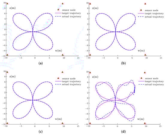
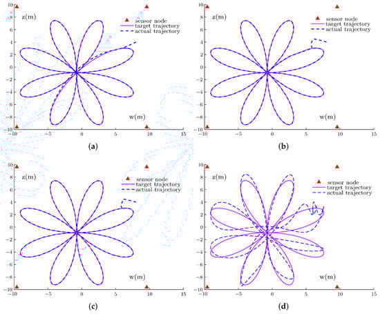
Figure 8 shows the target trajectory and actual trajectory for positioning employing FPDP model with AF (5), FPDP model with AF (10), the VPDP model, and the pseudo-inverse method under sine noise ${\eta }_l\left(t\right)=sin(4\pi t+\pi )$. Figure 9 shows the error $\parallel y\left(t\right)-y^{*}{\left(t\right)\parallel }_2$ of these models. As shown in Figure 8, the target trajectory and the actual trajectory are basically coincident for all models except the pseudo-inverse method. In addition, a significant gap between these methods exists in convergence time from Figure 9. To be more specific, except for the pseudo-inverse method that cannot converge, the convergence time of FPDP model with AF (5), FPDP model with AF (10), and the VPDP model is 1.05 s, 0.6 s, 0.15 s. Besides, the error upper bounds of the VPDP model, FPDP model with AF (5), and FPDP model with AF (10), are about $9.5\times {10}^{-3}$, $9.5\times {10}^{-3}$, $9\times {10}^{-2}$, respectively. It is indicative that the VPDP model is superior to other two FPDP models. To sum up, this demonstrates the effectiveness of design formula (11) in realizing plane positioning issue.

Figure 8. The target trajectories and actual trajectories by the two FPDP models, VPDP model and the pseudo-inverse method with noise ${\eta }_l\left(t\right)=sin(4\pi t+\pi )$. (a) FPDP model with AF (5). (b) FPDP model with AF (10). (c) VPDP model with AF (12). (d) The pseudo-inverse method.

Figure 9. Dynamic characteristics of the $\parallel y\left(t\right)-y^{*}{\left(t\right)\parallel }_2$ by the two FPDP models, VPDP model, and the pseudo-inverse method with noise ${\eta }_l\left(t\right)=sin(4\pi t+\pi )$. (a) FPDP model with AF (5). (b) FPDP model with AF (10). (c) VPDP model with AF (12). (d) The pseudo-inverse method.

5.4. Example 2

In this example, the four sensor nodes coordinates are the same as in Section 5.3. Besides, the specified target trajectory $y^{*}\left(t\right)={[w^{*}\left(t\right),z^{*}\left(t\right)]}^{\mathrm{T}}$ is

$$\begin{array}{c}\hfill 9\left[\begin{array}{c}cos(2\pi {sin}^2(\pi t/12)+\pi /6)sin(8\pi {sin}^2(\pi t/12)+2\pi /3)-cos(\pi /6)sin(2\pi /3)+2\\ sin(2\pi {sin}^2(\pi t/12)+\pi /6)sin(8\pi {sin}^2(\pi t/12)+2\pi /3)-sin(\pi /6)sin(2\pi /3)+1\end{array}\right].\end{array}$$

Take the initial position $y\left(0\right)={[8,4]}^{\mathrm{T}}$, $k_1=k_2=0.5$, $q=1/p=0.2$; the parameter of AF (10) is set as $k_5=0.2$; the parameters of AF (12) are set as ${\mu }_1=0$, ${\mu }_2=0.5$; variable parameters (13) are set as ${\lambda }_1={\lambda }_2=5$ and ${\phi }_1={\phi }_2=0.5$.

Figure 10 shows the target trajectory and actual trajectory for positioning and employing the FPDP model with AF (5), the FPDP model with AF (10), the VPDP model, and the pseudo-inverse method under sine noise ${\eta }_l\left(t\right)=sin(4\pi t+\pi )$. Figure 11 shows the error $\parallel y\left(t\right)-y^{*}{\left(t\right)\parallel }_2$ of these models. As shown in Figure 10, the target trajectory and the actual trajectory are basically coincident for all models except for the pseudo-inverse method. Besides, a significant gap between these methods exists in convergence time from Figure 11. Specifically, except for the pseudo-inverse method that cannot converge, the convergence time of FPDP model with AF (5), FPDP model with AF (10), and the VPDP model is 1.82 s, 0.85 s, 0.26 s. Furthermore, the error upper bounds of the VPDP model, FPDP model with AF (5), and FPDP model with AF (10) are the same as in Figure 9. It is indicate that the VPDP model is better than the other two FPDP models, even for different target trajectory positioning tasks.

Figure 10. The target trajectories and actual trajectories by the two FPDP models, VPDP model, and the pseudo-inverse method with noise ${\eta }_l\left(t\right)=sin(4\pi t+\pi )$. (a) FPDP model with AF (5). (b) FPDP model with AF (10). (c) VPDP model with AF (12). (d) The pseudo-inverse method.

Figure 11. Dynamic characteristics of the $\parallel y\left(t\right)-y^{*}{\left(t\right)\parallel }_2$ by the two FPDP models, VPDP model and the pseudo-inverse method with noise ${\eta }_l\left(t\right)=sin(4\pi t+\pi )$. (a) FPDP model with AF (5). (b) FPDP model with AF (10). (c) VPDP model with AF (12). (d) The pseudo-inverse method.

6. Conclusions

In this paper, the DAZNN model (14) with exponential decay variable parameters (13) and exponential-type SBPAF (12) is proposed to solve the dynamic matrix inversion problem. The ETSBPAF and variable parameters (13) contribute positively to the convergence and robustness of the model, resulting in better performance when compared with the other mentioned fixed-parameter models. Furthermore, Theorem 1 theoretically establishes the upper bounds of convergence for the DAZNN model (14) with arbitrary time. As bounded additive noise is added, the robustness of the DAZNN model is theoretically demonstrated in Theorem 2. The results indicate that the DAZNN model has better performance than other models with various AFs based upon the three aspects of convergence, robustness, and initial value sensitivity. Finally, the AOA dynamic positioning example that employs evolution formula (11) of the DAZNN model verifies its availability. A simplified model with high performance may be considered in future research. Additionally, by using drones for assistance in positioning, dynamic positioning tasks can be extended to three dimensions.

References

- Stefanovski, J. Novel all-pass factorization, all solutions to rational matrix equation and control application. IEEE Trans. Autom. Control 2019, 65, 3176–3183. [Google Scholar] [CrossRef]
- Xiao, L.; Liu, S.; Wang, X.; He, Y.; Jia, L.; Xu, Y. Zeroing neural networks for dynamic quaternion-valued matrix inversion. IEEE Trans. Ind. Inform. 2021, 18, 1562–1571. [Google Scholar] [CrossRef]
- Quan, Z.; Liu, J. Efficient complex matrix inversion for MIMO OFDM systems. J. Commun. Netw. 2017, 19, 637–647. [Google Scholar] [CrossRef]
- Wang, Y.; Leib, H. Sphere decoding for MIMO systems with Newton iterative matrix inversion. IEEE Commun. Lett. 2013, 17, 389–392. [Google Scholar] [CrossRef]
- Guo, D.; Zhang, Y. Zhang neural network, Getz–Marsden dynamic system, and discrete-time algorithms for time-varying matrix inversion with application to robots’ kinematic control. Neurocomputing 2012, 97, 22–32. [Google Scholar] [CrossRef]
- Jin, L.; Zhang, Y. G2-type SRMPC scheme for synchronous manipulation of two redundant robot arms. IEEE Trans. Cybern. 2014, 45, 153–164. [Google Scholar] [PubMed]
- Chen, D.; Li, S.; Wu, Q.; Luo, X. Super-twisting ZNN for coordinated motion control of multiple robot manipulators with external disturbances suppression. Neurocomputing 2020, 371, 78–90. [Google Scholar] [CrossRef]
- Krishnamoorthy, A.; Menon, D. Matrix inversion using Cholesky decomposition. In Proceedings of the 2013 Signal Processing: Algorithms, Architectures, Arrangements, and Applications (SPA), Poznan, Poland, 26–28 September 2013; pp. 70–72. [Google Scholar]
- Tang, C.; Liu, C.; Yuan, L.; Xing, Z. High precision low complexity matrix inversion based on Newton iteration for data detection in the massive MIMO. IEEE Commun. Lett. 2016, 20, 490–493. [Google Scholar] [CrossRef]
- Xiao, L.; He, Y. A noise-suppression ZNN model with new variable parameter for dynamic Sylvester equation. IEEE Trans. Ind. Inform. 2021, 17, 7513–7522. [Google Scholar] [CrossRef]
- Stanimirović, P.S.; Živković, I.S.; Wei, Y. Recurrent neural network for computing the Drazin inverse. IEEE Trans. Neural Netw. Learn. Syst. 2015, 26, 2830–2843. [Google Scholar] [CrossRef] [PubMed]
- Elhoseny, M.; Shankar, K. Optimal bilateral filter and convolutional neural network based denoising method of medical image measurements. Measurement 2019, 143, 125–135. [Google Scholar] [CrossRef]
- Koyuncu, I.; Yilmaz, C.; Alcin, M.; Tuna, M. Design and implementation of hydrogen economy using artificial neural network on field programmable gate array. Int. J. Hydrogen Energy 2020, 45, 20709–20720. [Google Scholar] [CrossRef]
- Wrobel, K.; Doroz, R.; Porwik, P.; Naruniec, J.; Kowalski, M. Using a probabilistic neural network for lip-based biometric verification. Eng. Appl. Artif. Intell. 2017, 64, 112–127. [Google Scholar] [CrossRef]
- Yañez-Badillo, H.; Beltran-Carbajal, F.; Tapia-Olvera, R.; Favela-Contreras, A.; Sotelo, C.; Sotelo, D. Adaptive robust motion control of quadrotor systems using artificial neural networks and particle swarm optimization. Mathematics 2021, 9, 2367. [Google Scholar] [CrossRef]
- Khan, A.T.; Li, S.; Cao, X. Control framework for cooperative robots in smart home using bio-inspired neural network. Measurement 2021, 167, 108253. [Google Scholar] [CrossRef]
- Wang, S.; Zhang, H.; Zhang, W.; Zhang, H. Finite-time projective synchronization of Caputo type fractional complex-valued delayed neural networks. Mathematics 2021, 9, 1406. [Google Scholar] [CrossRef]
- Li, Y.; Liu, Y.; Tong, S. Observer-based neuro-adaptive optimized control of strict-feedback nonlinear systems with state constraints. IEEE Trans. Neural Netw. Learn Syst. 2021. [Google Scholar] [CrossRef] [PubMed]
- Cogollo, M.R.; González-Parra, G.; Arenas, A.J. Modeling and forecasting cases of RSV using artificial neural networks. Mathematics 2021, 9, 2958. [Google Scholar] [CrossRef]
- Šestanović, T.; Arnerić, J. Can recurrent neural networks predict inflation in euro zone as good as professional forecasters? Mathematics 2021, 9, 2486. [Google Scholar] [CrossRef]
- Simos, T.E.; Mourtas, S.D.; Katsikis, V.N. Time-varying Black–Litterman portfolio optimization using a bio-inspired approach and neuronets. Appl. Soft Comput. 2021, 112, 107767. [Google Scholar] [CrossRef]
- Katsikis, V.N.; Mourtas, S.D.; Stanimirović, P.S.; Li, S.; Cao, X. Time-varying mean–variance portfolio selection problem solving via LVI-PDNN. Comput. Oper. Res. 2022, 138, 105582. [Google Scholar] [CrossRef]
- Xiao, L. A new design formula exploited for accelerating Zhang neural network and its application to time-varying matrix inversion. Theor. Comput. Sci. 2016, 647, 50–58. [Google Scholar] [CrossRef]
- Xiao, L. A nonlinearly activated neural dynamics and its finite-time solution to time-varying nonlinear equation. Neurocomputing 2016, 173, 1983–1988. [Google Scholar] [CrossRef]
- Li, S.; Chen, S.; Liu, B. Accelerating a recurrent neural network to finite-time convergence for solving time-varying Sylvester equation by using a sign-bi-power activation function. Neural Process Lett. 2013, 37, 189–205. [Google Scholar] [CrossRef]
- Xiao, L. A finite-time convergent Zhang neural network and its application to real-time matrix square root finding. Neural Comput. Appl. 2019, 31, 793–800. [Google Scholar] [CrossRef]
- Yan, Z.; Zhong, S.; Lin, L.; Cui, Z. Adaptive Levenberg–Marquardt algorithm: A new optimization strategy for Levenberg–Marquardt neural networks. Mathematics 2021, 9, 2176. [Google Scholar] [CrossRef]
- Stanimirović, P.S.; Katsikis, V.N.; Li, S. Integration enhanced and noise tolerant ZNN for computing various expressions involving outer inverses. Neurocomputing 2019, 329, 129–143. [Google Scholar] [CrossRef]
- Li, W. Design and analysis of a novel finite-time convergent and noise-tolerant recurrent neural network for time-variant matrix inversion. IEEE Trans. Syst. Man Cybern. Syst. 2018, 50, 4362–4376. [Google Scholar] [CrossRef]
- Jin, L.; Zhang, Y.; Li, S.; Zhang, Y. Modified ZNN for time-varying quadratic programming with inherent tolerance to noises and its application to kinematic redundancy resolution of robot manipulators. IEEE Trans. Ind. Electron. 2016, 63, 6978–6988. [Google Scholar] [CrossRef]
- Xiao, L.; Zhang, Y.; Zuo, Q.; Dai, J.; Li, J.; Tang, W. A noise-tolerant zeroing neural network for time-dependent complex matrix inversion under various kinds of noises. IEEE Trans. Ind. Inform. 2019, 16, 3757–3766. [Google Scholar] [CrossRef] [Green Version]
- Hu, Z.; Xiao, L.; Dai, J.; Xu, Y.; Zuo, Q.; Liu, C. A Unified Predefined-Time Convergent and Robust ZNN Model for Constrained Quadratic Programming. IEEE Trans. Ind. Inform. 2020, 17, 1998–2010. [Google Scholar] [CrossRef]
- Shen, L.; Wu, J.; Yang, S. Initial position estimation in SRM using bootstrap circuit without predefined inductance parameters. IEEE Trans. Power Electr. 2011, 26, 2449–2456. [Google Scholar] [CrossRef]
- Li, W.; Su, Z.; Tan, Z. A variable-gain finite-time convergent recurrent neural network for time-variant quadratic programming with unknown noises endured. IEEE Trans. Ind. Inform. 2019, 15, 5330–5340. [Google Scholar] [CrossRef]
- Xiao, L.; Zhang, Y.; Dai, J.; Zuo, Q.; Wang, S. Comprehensive analysis of a new varying parameter zeroing neural network for time varying matrix inversion. IEEE Trans. Ind. Inform. 2020, 17, 1604–1613. [Google Scholar] [CrossRef]
- Stanimirović, P.; Gerontitis, D.; Tzekis, P.; Behera, R.; Sahoo, J.K. Simulation of varying parameter recurrent neural network with application to matrix inversion. Math. Comput. Simul. 2021, 185, 614–628. [Google Scholar] [CrossRef]
- Li, X.; Li, S.; Xu, Z.; Zhou, X. A vary-parameter convergence-accelerated recurrent neural network for online solving dynamic matrix pseudoinverse and its robot application. Neural Process Lett. 2021, 53, 1287–1304. [Google Scholar] [CrossRef]
- Zhang, Y.; Jiang, D.; Wang, J. A recurrent neural network for solving Sylvester equation with time-varying coefficients. IEEE Trans. Neural Netw. 2002, 13, 1053–1063. [Google Scholar] [CrossRef] [PubMed]
- Zhang, Y.; Qiu, B.; Jin, L.; Guo, D.; Yang, Z. Infinitely many Zhang functions resulting in various ZNN models for time-varying matrix inversion with link to Drazin inverse. Inf. Process. Lett. 2015, 115, 703–706. [Google Scholar] [CrossRef]
- Xiao, L.; Tan, H.; Jia, L.; Dai, J.; Zhang, Y. New error function designs for finite-time ZNN models with application to dynamic matrix inversion. Neurocomputing 2020, 402, 395–408. [Google Scholar] [CrossRef]
- Zhang, Y.; Chen, K. Comparison on Zhang neural network and gradient neural network for time-varying linear matrix equation AXB=C solving. In Proceedings of the 2008 IEEE International Conference on Industrial Technology, Chengdu, China, 21–24 April 2008; pp. 1–6. [Google Scholar]
- Miao, P.; Shen, Y.; Xia, X. Finite time dual neural networks with a tunable activation function for solving quadratic programming problems and its application. Neurocomputing 2014, 143, 80–89. [Google Scholar] [CrossRef] [Green Version]
- Li, W.; Liao, B.; Xiao, L.; Lu, R. A recurrent neural network with predefined-time convergence and improved noise tolerance for dynamic matrix square root finding. Neurocomputing 2019, 337, 262–273. [Google Scholar] [CrossRef]
- Dai, J.; Li, Y.; Xiao, L.; Jia, L. Zeroing neural network for time-varying linear equations with application to dynamic positioning. IEEE Trans. Ind. Inform. 2021. [Google Scholar] [CrossRef]
Publisher’s Note: MDPI stays neutral with regard to jurisdictional claims in published maps and institutional affiliations. |
© 2021 by the authors. Licensee MDPI, Basel, Switzerland. This article is an open access article distributed under the terms and conditions of the Creative Commons Attribution (CC BY) license (https://creativecommons.org/licenses/by/4.0/).