Comparison of Risk Ratios of Shrinkage Estimators in High Dimensions

Abstract

In this paper, we analyze the risk ratios of several shrinkage estimators using a balanced loss function. The James–Stein estimator is one of a group of shrinkage estimators that has been proposed in the existing literature. For these estimators, sufficient criteria for minimaxity have been established, and the James–Stein estimator’s minimaxity has been derived. We demonstrate that the James–Stein estimator’s minimaxity is still valid even when the parameter space has infinite dimension. It is shown that the positive-part version of the James–Stein estimator is substantially superior to the James–Stein estimator, and we address the asymptotic behavior of their risk ratios to the maximum likelihood estimator (MLE) when the dimensions of the parameter space are infinite. Finally, a simulation study is carried out to verify the performance evaluation of the considered estimators.

1. Introduction

When it comes to estimating the mean parameter of a multivariate normal distribution, the minimax technique has attracted the greatest attention and development in research thus far. Following Stein [1], it is well-known that the maximum likelihood estimator (MLE) is minimax and admissible when the dimensions of the parameter space are less than or equal to two. On the other hand, the MLE maintains the minimax property but is no longer admissible when the dimension is greater than three. Therefore, enhancing estimators has been accomplished through the development of shrinkage estimators that minimize the risk associated with the quadratic loss function. The efficient outperformance of these shrinkage estimators, compared to the MLE, has been demonstrated in various studies; for example, see Baranchik [2], Efron and Morris [3,4], Stein [5], Casella and Whang [6], Berger [7], Arnold [8], and Gruber [9]. Stein [1] and James and Stein [10] have also provided specific suggestions for improvement. In this paper, we discuss adaptive shrinkage estimating strategies and show how they may be generated by shrinking a raw estimate. In addition, we report our investigation of the characteristics of several shrinkage estimators in the context of risk.

There have been various recent studies focused on shrinkage estimation, including those of Nourouzirad and Arashi [11], Nimet and Selahettin [12], Kashari et al. [13], and Benkhaled and Hamdaoui [14]. Shrinkage estimators for multivariate normal means in the Bayesian framework have been examined by Hamdaoui et al. [15], in order to determine the minimaxity and limitations of their risk ratios. For the $X~N_d(\theta , {\sigma }^2 I_d)$ model, the authors used the prior law $\theta ~N_d(\upsilon , {\tau }^2 I_d)$, in which the parameters $\upsilon$ and ${\tau }^2$ are known but the parameter ${\sigma }^2$ is unknown. They developed two modified Bayes estimators, a ${\delta }_B^{\ast }$ and an empirical ${\delta }_{EB}^{\ast }$. When the sample size $n$ and the dimension of parameter space $d$ are finite, they found that the estimators ${\delta }_B^{\ast }$ and ${\delta }_{EB}^{\ast }$ are minimax under the quadratic loss. When $n$ and $d$ approach infinity, the risk ratios of these estimators were examined in terms of the MLE $X$.

Improvement of the estimators can also be achieved by incorporating a balanced loss function. Zellner [16] presented a balanced loss function that is intended to represent two requirements; namely, quality of fit and accuracy of the estimate. We refer to Farsipour and Asgharzadeh [17], Karamikabir et al. [18], and Selahattin and Issam [19] for further information on the use of this loss function. Using the generalized Bayes shrinkage estimators of location parameter for a spherical distribution subject to a balance-type loss, Karamikabir et al. [20] determined the minimax and acceptable estimators of the location parameter.

In this paper, we use the model $Y~N_d(\mu , {\tau }^2 I_d)$, in which the parameter $\tau$ is well known. Our main purpose was to estimate the unknown parameter $\mu$, by using shrinkage estimators derived from the MLE to solve for $\mu$. We utilized the risk associated with the balanced loss function to compare two estimators. With the incorporation of the balanced loss function, the risk function of the estimators was computed using $T_{\alpha }({\Vert Y\Vert }^2)=(1-\alpha \frac{1}{{\Vert Y\Vert }^2})Y$, where the real constant $\alpha$ may be dependent on $d$, and $\Vert .\Vert$ is the typical norm in ${ℝ}^d$. In addition, we investigated the minimaxity characteristic of the estimators and concluded that the James–Stein estimator has the same feature. We also extended the work to study the limit of the risk ratios of the James–Stein estimator to the MLE when $d$ tends to infinity. We discuss the positive-part version of the James–Stein estimator and the asymptotic behavior of its risk ratios to the MLE in scenarios where the dimension of the parameter space $d$ is either finite or goes to infinity. We demonstrate that, when $d$ is finite, the positive-part version of the James–Stein estimator outperforms the James–Stein estimator.

The remainder of this paper is structured as follows: In Section 2, we present our model and recall some published findings that are useful in proving the main results. In Section 3, we show the minimaxity property and the limit of the risk ratios of the James–Stein estimator and its positive-part version, regarding the dimension of the parameter space. We end this paper with the results of a simulation study, which illustrate the performance of the considered estimators.

2. Model Presentations

In this section, we recall that, if $U$ is a multivariate Gaussian random variable $N_d(\mu , {\tau }^2 I_d)$ in ${ℝ}^d$, then $\frac{{\Vert U\Vert }^2}{{\tau }^2}~{\chi }_d^2(\frac{{\Vert \mu \Vert }^2}{{\tau }^2})$, where ${\chi }_d^2(\frac{{\Vert \mu \Vert }^2}{{\tau }^2})$ denotes the non-central chi-square distribution with $d$ degrees of freedom and non-centrality parameter $\frac{{\Vert \mu \Vert }^2}{{\tau }^2}$.

Suppose that $Z$ is a random vector which follows a multivariate normal distribution $N_d(\mu , {\tau }^2 I_d)$, where the parameter $\mu$ is unknown. For any estimator $T$ of the parameter $\mu$, the balanced squared error loss function of $T$ can then be defined as

$${\ell }_{\omega }(T,\mu )=\omega {\Vert T-T_0\Vert }^2+(1-\omega ){\Vert T-\mu \Vert }^2,$$

(1)

where $T$ is the given estimator that is being compared to the target estimator $T_0$ of $\mu$, $\omega$ is the weight provided to the closeness of $T$ to $T_0$, and $1-\omega$ is the relative weight given to the precision of the estimator $T$ to $\mu$. This means that the risk function associated with ${\ell }_{\omega }(T,\mu )$ is defined as follows:

$${ℛ}_{\omega }(T,\mu )=\omega E({\Vert T-T_0\Vert }^2)+(1-\omega )E({\Vert T-\mu \Vert }^2).$$

(2)

Now, considering the model $Z~N_d(\mu , {\tau }^2 I_d)$, in which ${\tau }^2$ is known, we focus on estimating the unknown mean parameter $\mu$ using shrinkage estimators under the balanced loss function defined in Equation (1). For simplicity, we only consider the scenario ${\tau }^2=1$, as any model of the type $Z~N_d(\mu , {\tau }^2 I_d)$ may be converted to a model $X~N_d(\mu , I_d)$ by a change of variables. Specifically, we investigate the estimation of the unknown parameter $\mu$ when $Y~N_d(\mu , I_d)$. In this case, following Benkhaled et al. [21], it is obvious that the MLE is $Y:=T_0$, and its risk function is ${ℛ}_{\omega }(T_0,\mu )=(1-\omega )d$. Therefore, any estimator that dominates $T_0$ is likewise minimax for $d\ge 3$.

For the proof given in the next section, we needed to address the result of Lemma 1 given in Stein [5], which states that

$$E((Z-\upsilon )f(Z))=E(f^{\prime }(Z)),$$

(3)

where $Z$ is a random variable that follows $N(\upsilon , 1)$, $f^{\prime }$ is the derivative of $f$, and $E(f^{\prime }(Z))<+\infty$.

3. Main Results

3.1. General Class of James–Stein Estimator

3.1.1. Risk Function and Minimaxity

Here, we study the minimaxity of estimators defined by

$$T_{\alpha }({\Vert Y\Vert }^2)=\left(1-\alpha \frac{1}{{\Vert Y\Vert }^2}\right)Y,$$

(4)

where $\alpha$ is a real parameter.

Proposition 1.

Under the balanced loss function${\ell }_{\omega }$given in Equation (1), the risk function of the estimator $T_{\alpha }({\Vert Y\Vert }^2)$ is

$${ℛ}_{\omega }(T_{\alpha }({\Vert Y\Vert }^2),\mu )=d(1-\omega )+\alpha (\alpha -2(1-\omega )(d-2))E\left(\frac{1}{{\Vert Y\Vert }^2}\right).$$

(5)

Proof of Proposition 1.

From Equations (2) and (4), we have

$$\begin{array}{ll}{ℛ}_{\omega }(T_{\alpha }({\Vert Y\Vert }^2),\mu )& =\omega E({\Vert T_{\alpha }({\Vert Y\Vert }^2)-T_0\Vert }^2)+(1-\omega )E({\Vert T_{\alpha }({\Vert Y\Vert }^2)-\mu \Vert }^2)\\ & =\omega E\left({\Vert -\alpha \frac{1}{{\Vert Y\Vert }^2}Y\Vert }^2\right)+(1-\omega )E\left({\Vert Y-\mu -\alpha \frac{1}{{\Vert Y\Vert }^2}Y\Vert }^2\right)\\ & ={\alpha }^{2}E\left(\frac{1}{{\Vert Y\Vert }^2}\right)+(1-\omega )E({\Vert Y-\mu \Vert }^2)\\ & -2(1-\omega )\alpha E(Y-\mu , \frac{1}{{\Vert Y\Vert }^2}Y).\end{array}$$

(6)

Using Equation (3), we obtain

$$\begin{gathered} E(<Y-\mu , \frac{1}{{\Vert Y\Vert }^2}Y>)=E\left({\displaystyle \sum }_{j=1}^d(Y_{j-}{\mu }_j)\frac{1}{{\Vert Y\Vert }^2}{Y}_j\right)={\displaystyle \sum }_{j=1}^{d}E\left[(Y_{j-}{\mu }_j)\frac{1}{{\Vert Y\Vert }^2}{Y}_j\right] \\ ={\displaystyle \sum }_{j=1}^{d}E\left[\frac{\partial }{\partial Y_j}\left(\frac{1}{{{\displaystyle \sum }}_{i=1}^d{Y}_i{}^2}{Y}_j\right)\right]=(d-2)E\left(\frac{1}{{\Vert Y\Vert }^2}\right). \end{gathered}$$

(7)

According to Equations (6) and (7), we obtain the desired result. □

Subsequently, from Equation (5), we can immediately deduce that a sufficient condition for the estimator $T_{\alpha }({\Vert Y\Vert }^2)$ to dominate the MLE $Y$ is

$$0\le \alpha \le 2(1-\omega )(d-2).$$

Due to the convexity of the risk function ${ℛ}_{\omega }(T_{\alpha }({\Vert Y\Vert }^2),\mu )$ on $\alpha$, the optimal value of $\alpha$ that minimizes this risk function is

$$\alpha =\widehat{\alpha }=(1-\omega )(d-2).$$

By replacing $\alpha$ with $\widehat{\alpha }$ in Equation (4), we then obtain the James–Stein estimator that is defined as

$$T_{J.S}({\Vert Y\Vert }^2)=\left(1-\frac{(1-\omega )(d-2)}{{\Vert Y\Vert }^2}\right)Y.$$

(8)

Additionally, its risk function related to the balanced loss function ${\ell }_{\omega }$ given in Equation (1) is given by

$${ℛ}_{\omega }(T_{J.S}({\Vert Y\Vert }^2),\mu )=d(1-\omega )-{(d-2)}^2{(1-\omega )}^{2}E\left(\frac{1}{{\Vert Y\Vert }^2}\right)$$

(9)

$$\le {ℛ}_{\omega }(T_0,\mu ).$$

We can then deduce that the James–Stein estimator $T_{J.S}({\Vert Y\Vert }^2)$ dominates the MLE; thus, $T_{J.S}({\Vert Y\Vert }^2)$ is minimax.

3.1.2. Asymptotic Behavior of Risk Ratios of James–Stein Estimator

This section discusses the effectiveness of the James–Stein estimator, in terms of dominating the MLE under the balanced loss function when the dimension of the parameter space $d$ goes to infinity.

Casella and Whang [6] have shown that the James–Stein estimator dominates the MLE under the quadratic loss function; that is, in the specific case of the balanced loss defined by Equation (1): $\omega =0$.

Theorem 1.

Under the balanced loss function${\ell }_{\omega }$defined in Equation (1), if $\underset{d\to +\infty }{lim}\frac{{\Vert \mu \Vert }^2}{d}=Q (Q>0)$, we get

$$\underset{d\to +\infty }{\lim }\frac{{ℛ}_{\omega }(T_{J.S}({\Vert Y\Vert }^2),\mu )}{{ℛ}_{\omega }(T_0,\mu )}=\frac{\omega +Q}{1+Q}.$$

Proof of Theorem 1.

From Lemma 1 of Casella and Whang [6], and for $d\ge 3,$ we have

$$\frac{1}{d-2+{\Vert \mu \Vert }^2}\le E\left(\frac{1}{{\Vert Y\Vert }^2}\right)\le \frac{1}{d-2}\left(\frac{d}{d+{\Vert \mu \Vert }^2}\right).$$

(10)

Using Equations (9) and (10), we obtain

$$1-\frac{(1-\omega )(d-2)}{d+{\Vert \mu \Vert }^2}\le \frac{{ℛ}_{\omega }(T_{J.S}({\Vert Y\Vert }^2),\mu )}{{ℛ}_{\omega }(T_0,\mu )}\le 1-\frac{(1-\omega ){(d-2)}^2}{d(d-2+{\Vert \mu \Vert }^2)}.$$

By passing to the limit—namely, when $d$ tends to infinity and under the condition $\underset{d\to +\infty }{\lim }\frac{{\Vert \mu \Vert }^2}{d}=Q (Q>0)—$we get

$$1-\underset{d\to +\infty }{\lim }\frac{(1-\omega )(d-2)}{d+{\Vert \mu \Vert }^2}\le \underset{d\to +\infty }{\lim }\frac{{ℛ}_{\omega }(T_{J.S}({\Vert Y\Vert }^2),\mu )}{{ℛ}_{\omega }(T_0,\mu )}\le 1-\underset{d\to +\infty }{\lim }\frac{(1-\omega ){(d-2)}^2}{d(d-2+{\Vert \mu \Vert }^2)},$$

and then

$$1-\underset{d\to +\infty }{\lim }\frac{\frac{(1-\omega )(d-2)}{d}}{\frac{d}{d}+\frac{{\Vert \mu \Vert }^2}{d}}\le \underset{d\to +\infty }{\lim }\frac{{ℛ}_{\omega }(T_{J.S}({\Vert Y\Vert }^2),\mu )}{{ℛ}_{\omega }(T_0,\mu )}\le 1-\underset{d\to +\infty }{\lim }\frac{\frac{(1-\omega ){(d-2)}^2}{d^2}}{\frac{d}{d}\left(\frac{d-2}{d}+\frac{{\Vert \mu \Vert }^2}{d}\right)}.$$

Thus,

$$\frac{\omega +Q}{1+Q}=1-\frac{1-\omega }{1+Q}\le \underset{d\to +\infty }{\lim }\frac{{ℛ}_{\omega }(T_{J.S}({\Vert Y\Vert }^2),\mu )}{{ℛ}_{\omega }(T_0,\mu )}\le 1-\frac{1-\omega }{1+Q}=\frac{\omega +Q}{1+Q},$$

Therefore,

$$\underset{d\to +\infty }{\lim }\frac{{ℛ}_{\omega }(T_{J.S}({\Vert Y\Vert }^2),\mu )}{{ℛ}_{\omega }(T_0,\mu )}=\frac{\omega +Q}{1+Q}<1 ,$$

as $0\le \omega <1$. This means that, even if $d$ tends to infinity, the James–Stein estimator $T_{J.S}({\Vert Y\Vert }^2)$ is superior to the MLE $T_0$. As a result, the minimaxity feature of the James–Stein estimator $T_{J.S}({\Vert Y\Vert }^2)$ remains stable. □

3.2. The Positive-Part Version of the James–Stein Estimator

In this section, we study the superiority of the positive-part version of the James–Stein estimator to the James–Stein estimator, and the limit of the risk ratio of the positive-part version of the James–Stein estimator to the MLE when the dimension of the parameter space $d$ tends to infinity. The positive-part version of James–Stein estimator is given by

$$T_{J.S+}({\Vert Y\Vert }^2)={\left(1-\frac{(1-\omega )(d-2)}{{\Vert Y\Vert }^2}\right)}^{+}Y,$$

(11)

where ${\left(1-\frac{(1-\omega )(d-2)}{{\Vert Y\Vert }^2}\right)}^{+}=\max \left(0,1-\frac{(1-\omega )(d-2)}{{\Vert Y\Vert }^2}\right)=\left(0,1-\frac{(1-\omega )(d-2)}{{\Vert Y\Vert }^2}\right){\mathbb{I}}_{\frac{(1-\omega )(d-2)}{{\Vert Y\Vert }^2}\le 1}$, with ${\mathbb{I}}_{\frac{ (1-\omega )(d-2)}{{\Vert Y\Vert }^2}\le 1}$ denoting the indicator function of the set $\left(\frac{ (1-\omega )(d-2)}{{\Vert Y\Vert }^2}\le 1\right)$.

3.2.1. Comparison of Risk Functions of the Positive-Part Version of the James–Stein Estimator and the James–Stein Estimator

Proposition 2.

Under the balanced loss function${\ell }_{\omega }$defined in Equation (1), the positive-part version of James–Stein estimator $T_{J.S+}$ defined in Equation (11) dominates the James–Stein estimator $T_{J.S}$ given in Equation (8).

Proof of Proposition 2.

We have

$${ℛ}_{\omega }(T_{J.S+}({\Vert Y\Vert }^2),\mu )=\omega E\left({\Vert T_{J.S+}({\Vert Y\Vert }^2)-T_0\Vert }^2\right)+(1-\omega )E\left({\Vert T_{J.S+}({\Vert Y\Vert }^2)-\mu \Vert }^2\right).$$

(12)

Baranchick [2] has shown that, under the quadratic loss function (i.e., in the case where $\omega =0$),

$$E\left({\Vert T_{J.S+}({\Vert Y\Vert }^2)-\mu \Vert }^2\right)\le E\left({\Vert T_{J.S}({\Vert Y\Vert }^2)-\mu \Vert }^2\right) \mathrm{for} \mathrm{any} \mu \in {ℝ}^d .$$

(13)

If $\omega =0,$ the positive–part version of James–Stein estimator $T_{J.S+}({\Vert Y\Vert }^2)$ then dominates the James–Stein estimator $T_{J.S}({\Vert Y\Vert }^2).$ Thus, using Equations (12) and (13), a sufficient condition for which $T_{J.S+}({\Vert Y\Vert }^2)$ dominates $T_{J.S}({\Vert Y\Vert }^2)$ under the balanced loss function (i.e., $0\le \omega <1)$ is

$$E\left({\Vert T_{J.S+}({\Vert Y\Vert }^2)-T_0\Vert }^2\right)\le E\left({\Vert T_{J.S}({\Vert Y\Vert }^2)-T_0\Vert }^2\right).$$

We have

$$\begin{array}{ll}E(\Vert T_{J.S+}({\Vert Y\Vert }^2)& -T_0{\Vert }^2)=E({\Vert T_{J.S+}({\Vert Y\Vert }^2)-T_{J.S}({\Vert Y\Vert }^2)+T_{J.S}({\Vert Y\Vert }^2)-Y\Vert }^2)\\ & =E({\Vert T_{J.S+}({\Vert Y\Vert }^2)-T_{J.S}({\Vert Y\Vert }^2)\Vert }^2)+E({\Vert T_{J.S}({\Vert Y\Vert }^2)-Y\Vert }^2)\\ & +2E(<T_{J.S+}({\Vert Y\Vert }^2)-T_{J.S}({\Vert Y\Vert }^2),T_{J.S}({\Vert Y\Vert }^2)-Y>)\\ & =E\left({\Vert (\frac{(1-\omega )(d-2)}{{\Vert Y\Vert }^2}-1){\mathbb{I}}_{\frac{ (1-\omega )(d-2)}{{\Vert Y\Vert }^2}\ge 1}Y\Vert }^2\right)\\ & +E\left({\Vert T_{J.S}({\Vert Y\Vert }^2)-Y\Vert }^2\right)\\ & -2(1-\omega )(d-2)E(<(\frac{ (1-\omega )(d-2)}{{\Vert Y\Vert }^2}-1){\mathbb{I}}_{\frac{ (1-\omega )(d-2)}{{\Vert Y\Vert }^2}\ge 1},\frac{1}{{\Vert Y\Vert }^2}Y>).\end{array}$$

Subsequently,

$$\begin{array}{ll}E(\Vert T_{J.S+}({\Vert Y\Vert }^2)& -T_0{\Vert }^2)-E\left({\Vert T_{J.S}({\Vert Y\Vert }^2)-T_0\Vert }^2\right)\\ & =E\left({\Vert (\frac{(1-\omega )(d-2)}{{\Vert Y\Vert }^2}-1){\mathbb{I}}_{\frac{ (1-\omega )(d-2)}{{\Vert Y\Vert }^2}\ge 1}Y\Vert }^2\right)\\ & -2(1-\omega )(d-2)E(<(\frac{ (1-\omega )(d-2)}{{\Vert Y\Vert }^2}-1){\mathbb{I}}_{\frac{ (1-\omega )(d-2)}{{\Vert Y\Vert }^2}\ge 1}Y,\frac{1}{{\Vert Y\Vert }^2}Y>)\\ & =E\left[\right(\frac{1}{{\Vert Y\Vert }^2}({\Vert Y\Vert }^2-(1-\omega )(d-2))({\Vert Y\Vert }^2\\ & +(1-\omega )(d-2))){\mathbb{I}}_{{\Vert Y\Vert }^2-(1-\omega )(d-2)\le 0}]\le 0.\end{array}$$

Thus, $T_{J.S+}({\Vert Y\Vert }^2)$ dominates $T_{J.S}({\Vert Y\Vert }^2)$ for any $0\le \omega <1$. □

3.2.2. Limit of Risk Ratio of the Positive-Part Version of the James–Stein Estimator to the MLE

Theorem 2.

Under the balanced loss function${\ell }_{\omega }$defined in Equation (1), if $\underset{d\to +\infty }{lim}\frac{{\Vert \mu \Vert }^2}{d}=Q (Q>0)$, we get

$$\underset{d\to +\infty }{\lim }\frac{{ℛ}_{\omega }(T_{J.S+}({\Vert Y\Vert }^2),\mu )}{{ℛ}_{\omega }(T_0,\mu )}=\frac{\omega +Q}{1+Q}.$$

Proof of Theorem 2.

As $T_{J.S+}({\Vert Y\Vert }^2)$ dominates $T_{J.S}({\Vert Y\Vert }^2)$ for any $0\le \omega <1$, then ${ℛ}_{\omega }(T_{J.S+}({\Vert Y\Vert }^2),\mu )\le {ℛ}_{\omega }(T_{J.S}({\Vert Y\Vert }^2),\mu )$ for any $0\le \omega <1$ and for all $d\ge 3$ and $\mu \in {ℝ}^d$. Hence,

$$\underset{d\to +\infty }{\lim }\frac{{ℛ}_{\omega }(T_{J.S+}({\Vert Y\Vert }^2),\mu )}{{ℛ}_{\omega }(T_0,\mu )}\le \underset{d\to +\infty }{\lim }\frac{{ℛ}_{\omega }(T_{J.S}({\Vert Y\Vert }^2),\mu )}{{ℛ}_{\omega }(T_0,\mu )}=\frac{\omega +Q}{1+Q}.$$

(14)

To ensure that $T_{J.S+}({\Vert Y\Vert }^2)$ dominates the MLE as $d$ tends to infinity, it suffices to show that

$$\underset{d\to +\infty }{\lim }\frac{{ℛ}_{\omega }(T_{J.S+}({\Vert Y\Vert }^2),\mu )}{{ℛ}_{\omega }(T_0,\mu )}\ge \frac{\omega +Q}{1+Q}.$$

Using the same techniques as used in the proof of Lemma 5 in Benmansour and Hamdaoui [22], based on Lemma 2.1 of Shao and Strawderman [23], we obtain

$${ℛ}_{\omega }(T_{J.S+}({\Vert Y\Vert }^2),\mu )={ℛ}_{\omega }(T_{J.S}({\Vert Y\Vert }^2),\mu )+E\left[\right({\Vert Y\Vert }^2+\frac{ {(1-\omega )}^2{(d-2)}^2}{{\Vert Y\Vert }^2}-d\left){\mathbb{I}}_{\frac{ (1-\omega )(d-2)}{{\Vert Y\Vert }^2}\ge 1}\right].$$

(15)

As

$$E\left({\Vert Y\Vert }^2{\mathbb{I}}_{\frac{(1-\omega )(d-2)}{{\Vert Y\Vert }^2}\ge 1}\right)={{\displaystyle \int }}_0^{+\infty }t{\mathbb{I}}_{\frac{(1-\omega )(d-2)}{t}\ge 1}{\chi }_d^2({\Vert \mu \Vert }^2)dt ,$$

where ${\chi }_d^2({\Vert \mu \Vert }^2)$ is the chi-squared distribution with $d$ degrees of freedom and non-centrality parameter ${\Vert \mu \Vert }^2$, and by applying Equation (1.3) in Casella and Hwang [6], we have

$$\begin{array}{ll}E\left({\Vert Y\Vert }^2{\mathbb{I}}_{\frac{(1-\omega )(d-2)}{{\Vert Y\Vert }^2}\ge 1}\right)& ={{\displaystyle \int }}_0^{+\infty }t{\mathbb{I}}_{\frac{(1-\omega )(d-2)}{t}\ge 1}{\chi }_d^2({\Vert \mu \Vert }^2)dt\\ & =d{{\displaystyle \int }}_0^{+\infty }{\mathbb{I}}_{\frac{(1-\omega )(d-2)}{t}\ge 1}{\chi }_{d+2}^2({\Vert \mu \Vert }^2)dt\\ & +2{\Vert \mu \Vert }^2{{\displaystyle \int }}_0^{+\infty }{\mathbb{I}}_{\frac{(1-\omega )(d-2)}{t}\ge 1}{\chi }_{d+4}^2({\Vert \mu \Vert }^2)dt\\ & =d\mathbb{P}({\chi }_{d+2}^2({\Vert \mu \Vert }^2)\le (1-\omega )(d-2))\\ & +2{\Vert \mu \Vert }^2\mathbb{P}({\chi }_{d+4}^2({\Vert \mu \Vert }^2)\le (1-\omega )(d-2)).\end{array}$$

(16)

Moreover,

$$\begin{gathered} E\left[\frac{{(1-\omega )}^2{(d-2)}^2}{{\Vert Y\Vert }^2}{\mathbb{I}}_{\frac{(1-\omega )(d-2)}{{\Vert Y\Vert }^2}\ge 1}\right]\ge \frac{1}{{(1-\omega )}^2{(d-2)}^2}E({\mathbb{I}}_{\frac{(1-\omega )(d-2)}{{\Vert Y\Vert }^2}\ge 1}) \\ \hspace{1em}\hspace{1em}\hspace{1em}\hspace{1em}\hspace{1em}=\frac{1}{{(1-\omega )}^2{(d-2)}^2}\mathbb{P}({\Vert Y\Vert }^2\le (1-\omega )(d-2)) \\ \hspace{1em}\hspace{1em}\hspace{1em}\hspace{1em}\hspace{1em}\hspace{1em}\hspace{1em}\hspace{1em}=\frac{1}{{(1-\omega )}^2{(d-2)}^2}\mathbb{P}({\chi }_d^2({\Vert \mu \Vert }^2)\le (1-\omega )(d-2)) , \end{gathered}$$

(17)

and

$$-dE\left[{\mathbb{I}}_{\frac{(1-\omega )(d-2)}{{\Vert Y\Vert }^2}\ge 1}\right]=-d\mathbb{P}({\chi }_d^2({\Vert \mu \Vert }^2)\le (1-\omega )(d-2)).$$

(18)

From Equations (16)–(18), we obtain

$$\begin{array}{ll}{ℛ}_{\omega }(T_{J.S+}({\Vert Y\Vert }^2),\mu )& \\ & \ge {ℛ}_{\omega }(T_{J.S}({\Vert Y\Vert }^2),\mu )+d \mathbb{P}({\chi }_{d+2}^2({\Vert \mu \Vert }^2)\le (1-\omega )(d-2))\\ & +2{\Vert \mu \Vert }^2 \mathbb{P}({\chi }_{d+4}^2({\Vert \mu \Vert }^2)\le (1-\omega )(d-2))\\ & +\frac{1}{(1-\omega )(d-2)}\mathbb{P}({\chi }_d^2({\Vert \mu \Vert }^2)\le (1-\omega )(d-2))\\ & -d\mathbb{P}({\chi }_d^2({\Vert \mu \Vert }^2)\le (1-\omega )(d-2)).\end{array}$$

Then,

$$\begin{array}{ll}\frac{{ℛ}_{\omega }(T_{J.S+}({\Vert Y\Vert }^2),\mu )}{{ℛ}_{\omega }(T_0,\mu )}& \\ & \ge \frac{{ℛ}_{\omega }(T_{J.S}({\Vert Y\Vert }^2),\mu )}{{ℛ}_{\omega }(T_0,\mu )}+\frac{d}{d(1-\omega )}\mathbb{P}({\chi }_{d+2}^2({\Vert \mu \Vert }^2)\le (1-\omega )(d-2))\\ & +\frac{2{\Vert \mu \Vert }^2}{d(1-\omega )}\mathbb{P}({\chi }_{d+4}^2({\Vert \mu \Vert }^2)\le (1-\omega )(d-2))\\ & +\frac{1}{d(d-2){(1-\omega )}^2}\mathbb{P}({\chi }_d^2({\Vert \mu \Vert }^2)\le (1-\omega )(d-2))\\ & -\frac{d}{d(1-\omega )}\mathbb{P}({\chi }_d^2({\Vert \mu \Vert }^2)\le (1-\omega )(d-2)).\end{array}$$

Using Equation (3.4) from Casella and Hwang [6], we have

$$\begin{array}{c}\underset{d\to +\infty }{\lim }\mathbb{P}({\chi }_{d+2}^2({\Vert \mu \Vert }^2)\le (1-\omega )(d-2))=\underset{d\to +\infty }{\lim } \mathbb{P}({\chi }_{d+4}^2({\Vert \mu \Vert }^2)\le (1-\omega )(d-2))\\ =\underset{d\to +\infty }{\lim } \mathbb{P}({\chi }_d^2({\Vert \mu \Vert }^2)\le (1-\omega )(d-2))=0.\end{array}$$

Subsequently, under the condition $\underset{d\to +\infty }{\lim }\frac{{\Vert \mu \Vert }^2}{d}=Q$, we obtain

$$\underset{d\to +\infty }{\lim }\frac{{ℛ}_{\omega }(T_{J.S+}({\Vert Y\Vert }^2),\mu )}{{ℛ}_{\omega }(T_0,\mu )}\ge \underset{d\to +\infty }{\lim }\frac{{ℛ}_{\omega }(T_{J.S}({\Vert Y\Vert }^2),\mu )}{{ℛ}_{\omega }(T_0,\mu )}=\frac{\omega +Q}{1+Q}.$$

(19)

According to Equations (14) and (19), we can deduce that

$$\underset{d\to +\infty }{\lim }\frac{{ℛ}_{\omega }(T_{J.S+}({\Vert Y\Vert }^2),\mu )}{{ℛ}_{\omega }(T_0,\mu )}=\frac{\omega +Q}{1+Q}\le 1;$$

namely, the positive-part version of James–Stein estimator $T_{J.S+}({\Vert Y\Vert }^2)$ dominates the MLE, even if $d$ tends to infinity. Thus, there is a stability of the minimaxity property of the positive-part version of the James–Stein estimator $T_{J.S+}({\Vert Y\Vert }^2)$ when the dimension of parameter space $d$ is in the neighborhood of infinity. □

4. Simulation Results

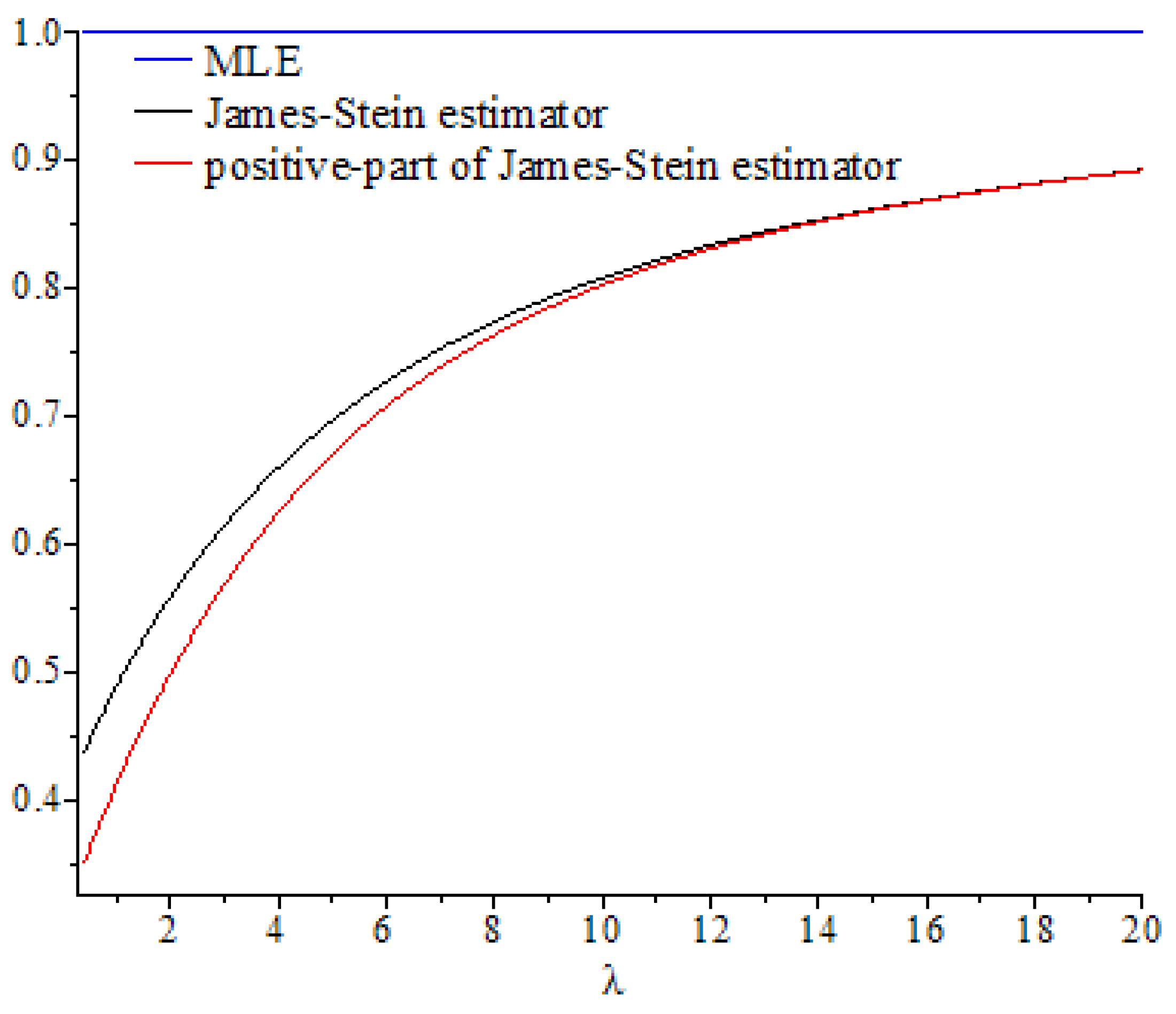
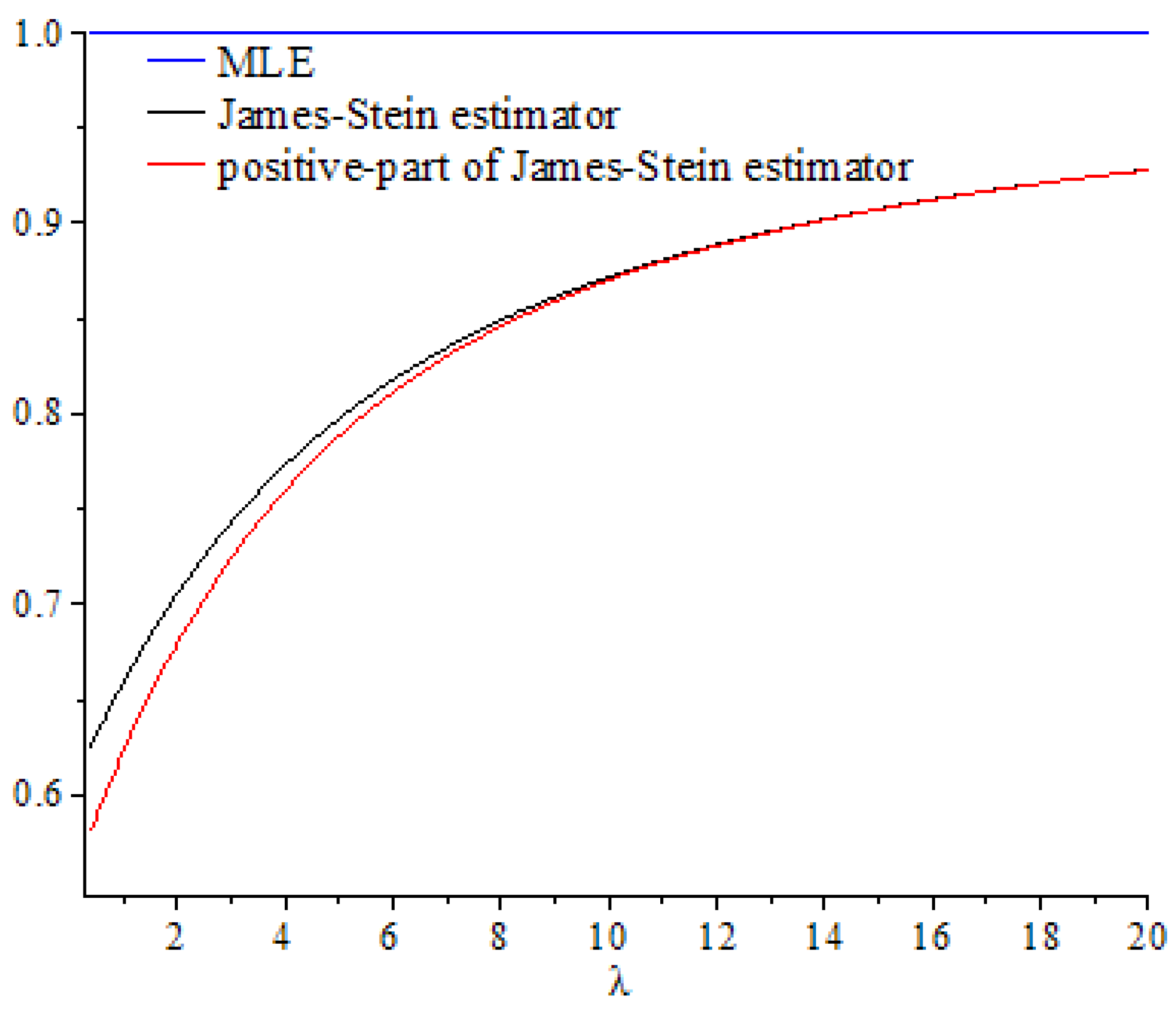
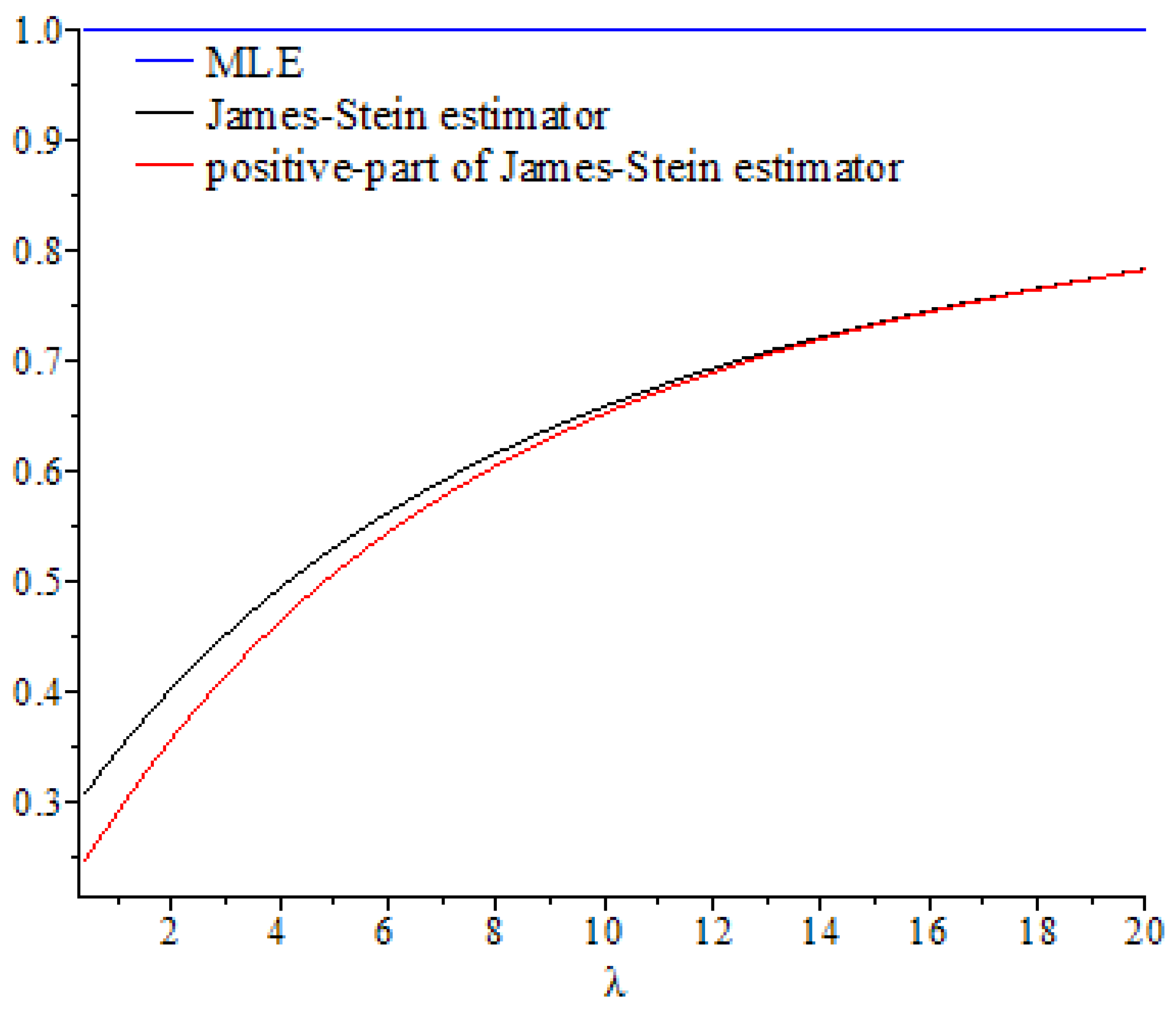
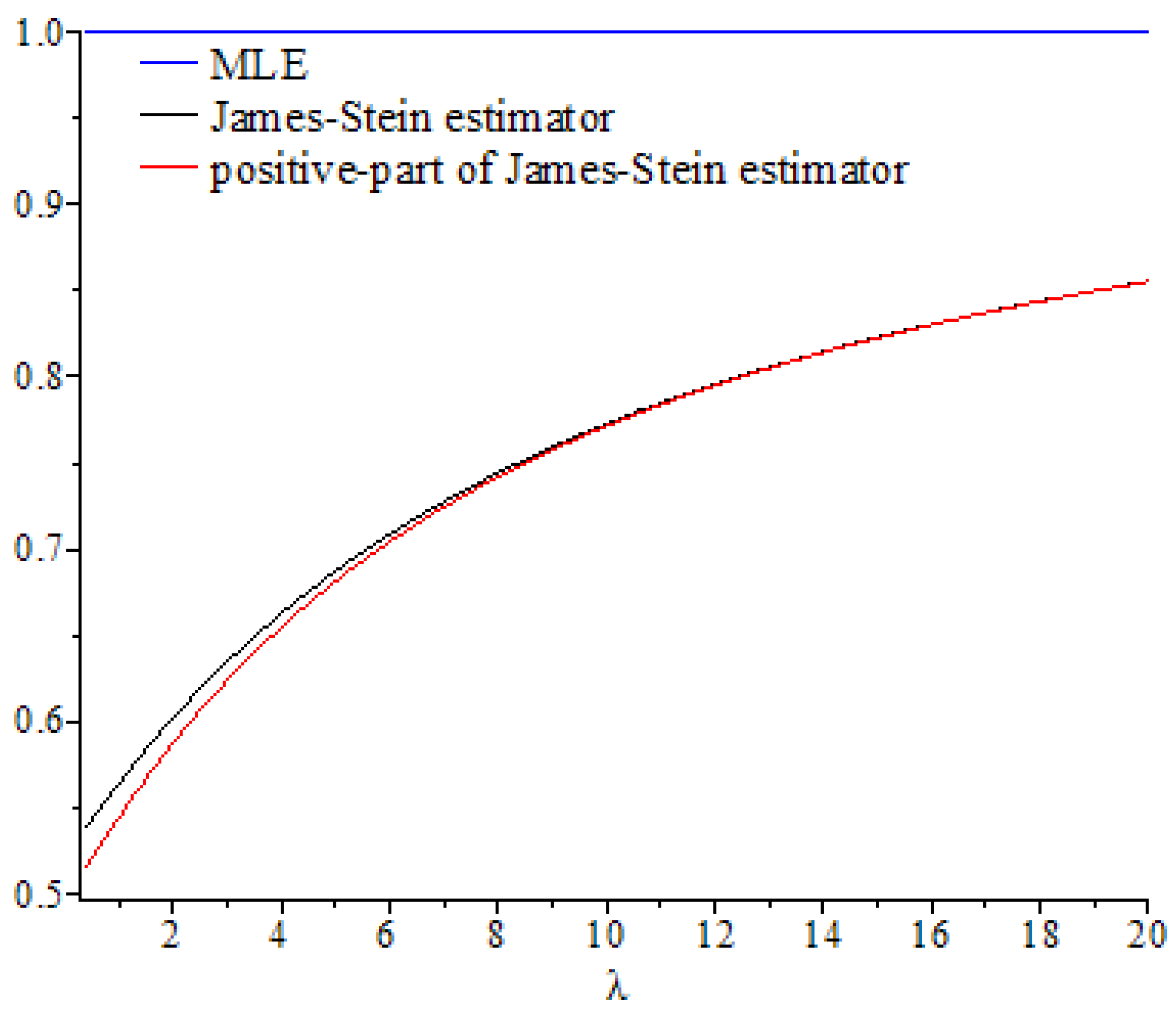
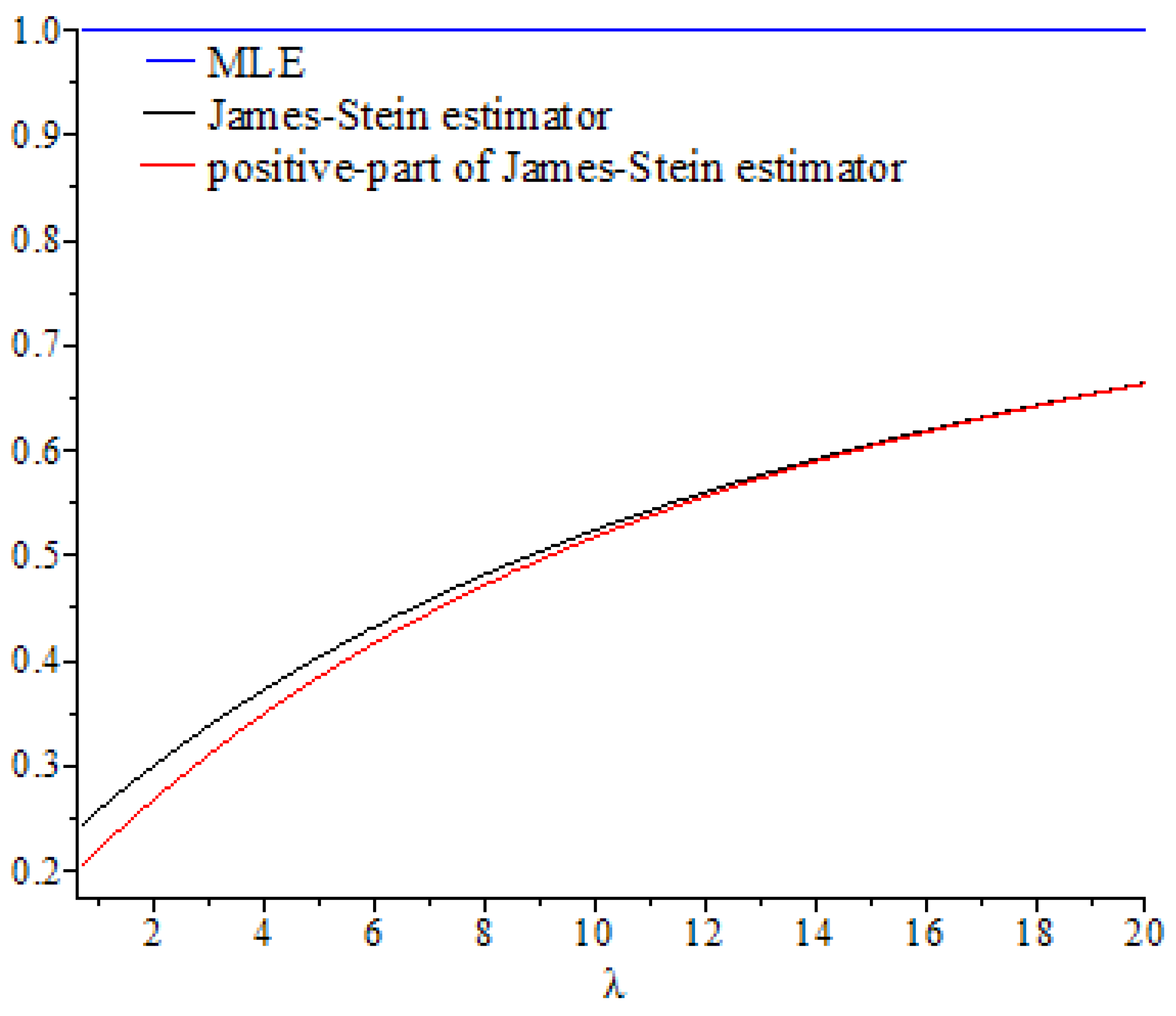
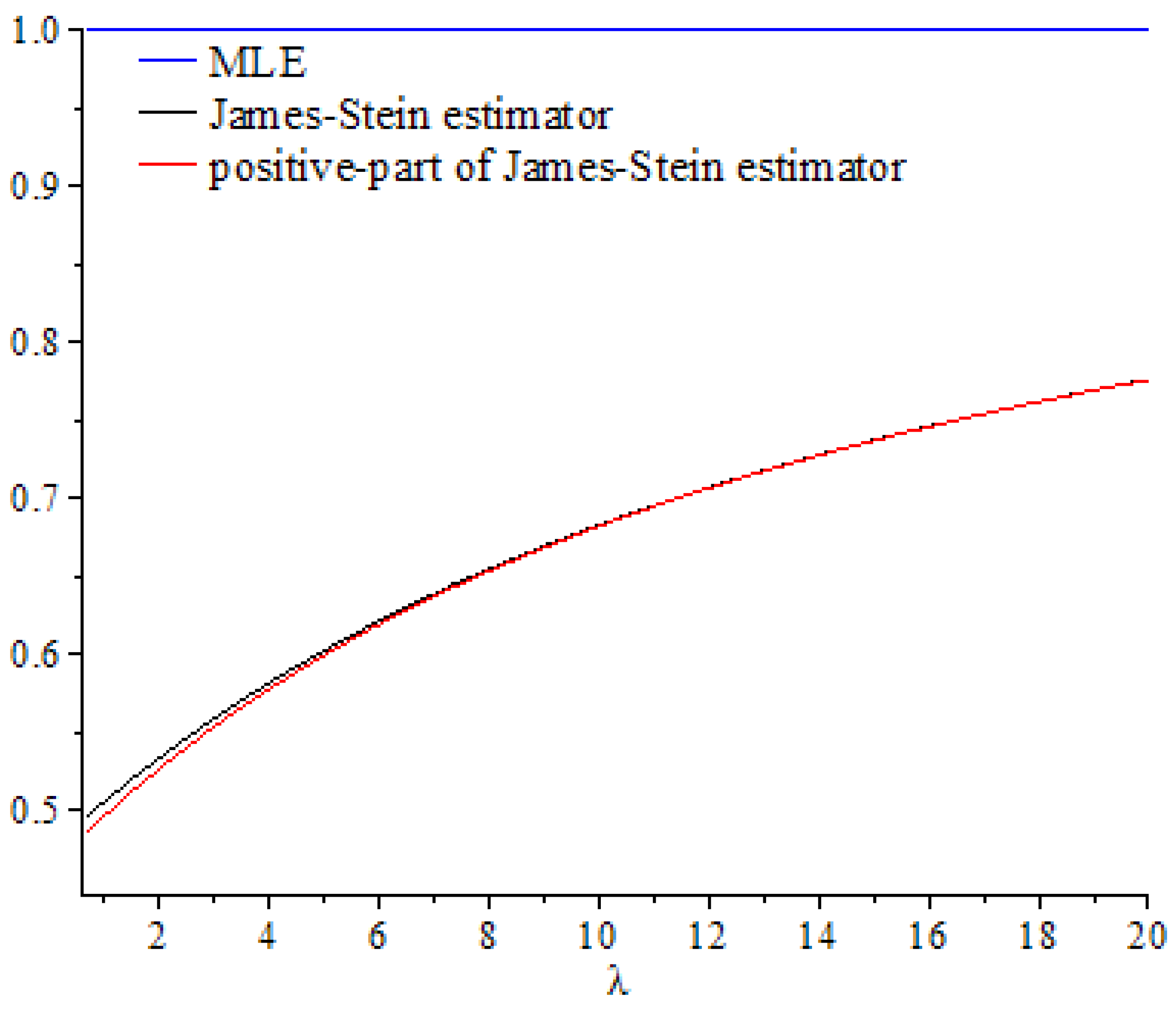
In this section, we discuss the values of the risk ratios of the James–Stein estimator $T_{J.S}({\Vert Y\Vert }^2)$ defined in Equation (8), for which the risk function under the balanced loss function is given by Equation (9), and the positive-part version of James–Stein estimator $T_{J.S+}({\Vert Y\Vert }^2)$ defined by Equation (11), for which the risk function related to the balanced loss function is given by Equation (15), with respect to the MLE. We denote these risk ratios as $\frac{{ℛ}_{\omega }(T_{J.S}({\Vert Y\Vert }^2),\mu )}{{ℛ}_{\omega }(T_0,\mu )}$ and $\frac{{ℛ}_{\omega }(T_{J.S+}({\Vert Y\Vert }^2),\mu )}{{ℛ}_{\omega }(T_0,\mu )}$, respectively. First, we discuss the performance of both estimators as functions of $\lambda ={\Vert \mu \Vert }^2$, and then compare their performance to the MLE based on selected values of the parameters $d$ and $\omega$. We then explain their performance based on various values of, $\omega$, and $\lambda ={\Vert \mu \Vert }^2.$

Figure 1, Figure 2, Figure 3, Figure 4, Figure 5 and Figure 6 show the curves of $\frac{{ℛ}_{\omega }(T_{J.S}({\Vert Y\Vert }^2),\mu )}{{ℛ}_{\omega }(T_0,\mu )}$ and $\frac{{ℛ}_{\omega }(T_{J.S+}({\Vert Y\Vert }^2),\mu )}{{ℛ}_{\omega }(T_0,\mu )}$ as functions of $\lambda ={\Vert \mu \Vert }^2$, based on selected values of the parameters $d$ and $\omega$. These curves were also compared to the gold standard curve of the risk ratio of the MLE (a constant function equal to 1). We noted that the values of the risk ratios $\frac{{ℛ}_{\omega }(T_{J.S}({\Vert Y\Vert }^2),\mu )}{{ℛ}_{\omega }(T_0,\mu )}$ and $\frac{{ℛ}_{\omega }(T_{J.S+}({\Vert Y\Vert }^2),\mu )}{{ℛ}_{\omega }(T_0,\mu )}$ were less than 1 for all selected values of $d$ and $\omega .$ This indicates that the James–Stein estimator $T_{J.S}({\Vert Y\Vert }^2)$ and the positive-part version of the James–Stein estimator $T_{J.S+}({\Vert Y\Vert }^2)$ are minimax. Furthermore, the estimators $T_{J.S}({\Vert Y\Vert }^2)$ and $T_{J.S+}({\Vert Y\Vert }^2)$ represented a significant improvement over the MLE, especially when the values of $\omega$ were close to zero and the dimension of the parameter space $d$ was high. Moreover, we noted a better performance of $T_{J.S+}({\Vert Y\Vert }^2)$, compared to $T_{J.S}({\Vert Y\Vert }^2)$, for the same values of $d$ and $\omega .$ By looking at the curves of both risk ratios, it can be seen that the risk ratio $\frac{{ℛ}_{\omega }(T_{J.S+}({\Vert Y\Vert }^2),\mu )}{{ℛ}_{\omega }(T_0,\mu )}$ was obviously lower than that of $\frac{{ℛ}_{\omega }(T_{J.S}({\Vert Y\Vert }^2),\mu )}{{ℛ}_{\omega }(T_0,\mu )}$ for most values of $\lambda$. The difference between these curves was significant for small values of $\lambda$ and negligible for larger values. This indicates that the improvement of $T_{J.S+}({\Vert Y\Vert }^2)$ over $T_{J.S}({\Vert Y\Vert }^2)$ was slight for large values of $\lambda$, and the curves of their risk ratios were almost identical once $\lambda$ exceeded a certain value. All results discussed through these figures can be confirmed by the values of risk ratios $\frac{{ℛ}_{\omega }(T_{J.S}({\Vert Y\Vert }^2),\mu )}{{ℛ}_{\omega }(T_0,\mu )}$ and $\frac{{ℛ}_{\omega }(T_{J.S+}({\Vert Y\Vert }^2),\mu )}{{ℛ}_{\omega }(T_0,\mu )}$ provided in

Table 1. Values of the risk ratios $\frac{{ℛ}_{\omega }(T_{J.S}({\Vert Y\Vert }^2),\mu )}{{ℛ}_{\omega }(T_0,\mu )}$ and $\frac{{ℛ}_{\omega }(T_{J.S+}({\Vert Y\Vert }^2),\mu )}{{ℛ}_{\omega }(T_0,\mu )}$ for $d=4$ and $\omega =0.1, 0.2, 0.5, 0.7, 0.9$ at different values of $\lambda ={\Vert \mu \Vert }^2$.

$\mathit{\lambda }$	$\mathit{\omega }=0.1$	$\mathit{\omega }=0.2$	$\mathit{\omega }=0.5$	$\mathit{\omega }=0.7$	$\mathit{\omega }=0.9$
1.2418	0.6648	0.7020	0.8138	0.8882	0.9627
	0.5826	0.6326	0.7809	0.8748	0.9611
1.6712	0.6950	0.7289	0.8305	0.8983	0.9661
	0.6229	0.6686	0.8028	0.8872	0.9647
3.7523	0.7969	0.8194	0.8871	0.9323	0.9774
	0.7601	0.7898	0.8750	0.9278	0.9769
5.0019	0.8348	0.8532	0.9082	0.9449	0.9816
	0.8108	0.8342	0.9009	0.9423	0.9814
10.4310	0.9142	0.9237	0.9523	0.9714	0.9905
	0.9108	0.9212	0.9515	0.9712	0.9904
20.0000	0.9550	0.9237	0.9523	0.9714	0.9905
	0.9549	0.9212	0.9515	0.9712	0.9904

,

Table 2. Values of the risk ratios $\frac{{ℛ}_{\omega }(T_{J.S}({\Vert Y\Vert }^2),\mu )}{{ℛ}_{\omega }(T_0,\mu )}$ and $\frac{{ℛ}_{\omega }(T_{J.S+}({\Vert Y\Vert }^2),\mu )}{{ℛ}_{\omega }(T_0,\mu )}$ for $d=10$ and $\omega =0.1, 0.2, 0.5, 0.7, 0.9$ at different values of $\lambda ={\Vert \mu \Vert }^2$.

$\mathit{\lambda }$	$\mathit{\omega }=0.1$	$\mathit{\omega }=0.2$	$\mathit{\omega }=0.5$	$\mathit{\omega }=0.7$	$\mathit{\omega }=0.9$
1.2418	0.3609	0.4319	0.6449	0.7870	0.9290
	0.3083	0.3914	0.6349	0.7855	0.9290
1.6712	0.3854	0.4567	0.6585	0.7951	0.9317
	0.3368	0.4169	0.6498	0.7939	0.9317
3.7523	0.4839	0.5413	0.7133	0.8280	0.9427
	0.4525	0.5190	0.7089	0.8274	0.9426
5.0019	0.5306	0.5827	0.7392	0.8435	0.9478
	0.5070	0.5666	0.7364	0.8432	0.9478
10.4310	0.6668	0.7039	0.8149	0.8889	0.9630
	0.6610	0.7003	0.8145	0.8889	0.9630
20.0000	0.7828	0.8070	0.8793	0.9276	0.9759
	0.7825	0.8068	0.8793	0.9276	0.9759

and

Table 3. Values of the risk ratios $\frac{{ℛ}_{\omega }(T_{J.S}({\Vert Y\Vert }^2),\mu )}{{ℛ}_{\omega }(T_0,\mu )}$ and $\frac{{ℛ}_{\omega }(T_{J.S+}({\Vert Y\Vert }^2),\mu )}{{ℛ}_{\omega }(T_0,\mu )}$ for $d=20$ and $\omega =0.1, 0.2, 0.5, 0.7, 0.9$ at different values of $\lambda ={\Vert \mu \Vert }^2$.

$\mathit{\lambda }$	$\mathit{\omega }=0.1$	$\mathit{\omega }=0.2$	$\mathit{\omega }=0.5$	$\mathit{\omega }=0.7$	$\mathit{\omega }=0.9$
1.6712	0.2529	0.3359	0.5849	0.7509	0.9170
	0.2245	0.3169	0.5831	0.7508	0.9169
2.4948	0.2807	0.3606	0.6004	0.7602	0.9201
	0.2558	0.3445	0.5991	0.7602	0.9201
3.7523	0.3196	0.3952	0.6220	0.7732	0.9244
	0.2991	0.3826	0.6211	0.7732	0.9244
5.0019	0.3545	0.4263	0.6414	0.7848	0.9283
	0.3380	0.4165	0.6408	0.7848	0.9283
10.4310	0.4739	0.5323	0.7077	0.8246	0.9415
	0.4681	0.5295	0.7076	0.8246	0.9415
20.0000	0.6054	0.6492	0.7808	0.8684	0.9561
	0.6047	0.6490	0.7807	0.8684	0.9561

for different set values of $\lambda ={\Vert \mu \Vert }^2$, $d$, and $\omega$. The first entry of each cell in these tables is the ratio $\frac{{ℛ}_{\omega }(T_{J.S}({\Vert Y\Vert }^2),\mu )}{{ℛ}_{\omega }(T_0,\mu )}$, while the second entry is the ratio $\frac{{ℛ}_{\omega }(T_{J.S+}({\Vert Y\Vert }^2),\mu )}{{ℛ}_{\omega }(T_0,\mu )}$.

The superiority of the James–Stein estimator $T_{J.S}({\Vert Y\Vert }^2)$ and the positive-part version of the James–Stein estimator $T_{J.S+}({\Vert Y\Vert }^2)$ over the MLE were observed under small values of both $\omega$ and $\lambda$. This improvement tended to decrease and approached zero as $\omega$ and $\lambda$ increased. We also observed that the improvement of both estimators and the dimension of the parameter space d were positively correlated under fixed values of $\omega$. We also noted that, for each value of $\lambda ={\Vert \mu \Vert }^2$, the values of the risk ratios $\frac{{ℛ}_{\omega }(T_{J.S}({\Vert Y\Vert }^2),\mu )}{{ℛ}_{\omega }(T_0,\mu )}$ and $\frac{{ℛ}_{\omega }(T_{J.S+}({\Vert Y\Vert }^2),\mu )}{{ℛ}_{\omega }(T_0,\mu )}$ tended to be identical for large values of $\omega$.

Hence, these results indicate the minimaxity of James–Stein estimator and the positive-part version of the James–Stein estimator, as well as the superiority of the positive-part version of the James–Stein estimator to the James–Stein estimator for different values of $d$ and $\omega$.

5. Conclusions

In this paper, we considered the estimation of the mean $\mu$ of a multivariate normal distribution $Y~N_d(\mu , I_d)$. We assessed the risk associated with the balanced loss function for comparing any two estimators. First, we established the minimaxity of the estimators defined by $T_{\alpha }({\Vert Y\Vert }^2)=(1-\alpha \frac{1}{{\Vert Y\Vert }^2})Y$, where $\alpha$ is a real parameter related to the dimension of the parameter space, $d$, and deduced the minimaxity of James–Stein estimator $T_{J.S}({\Vert Y\Vert }^2)$. When the value of $d$ was in the neighborhood of infinity, we studied the asymptotic behavior of risk ratios of the James–Stein estimator to the MLE. We then showed that, under the condition $\underset{d\to +\infty }{\lim }\frac{{\Vert \mu \Vert }^2}{d}=Q>0,$ the limit of the risk ratio $\frac{{ℛ}_{\omega }(T_{J.S}({\Vert Y\Vert }^2),\mu )}{{ℛ}_{\omega }(T_0,\mu )}$ tended to the value $\frac{\omega +Q}{1+Q}(\le 1)$; in other words, the James–Stein estimator $T_{J.S}({\Vert Y\Vert }^2)$ dominates the MLE, even when $d$ tends to infinity. Thus, the minimaxity property of the James–Stein estimator $T_{J.S}({\Vert Y\Vert }^2)$ remains stable, even if $d$ is in the neighborhood of infinity. Second, following the same steps as in the first part, we examined the minimaxity of the positive-part version of the James–Stein estimator $T_{J.S+}({\Vert Y\Vert }^2)$, in the case when $d$ is finite. When $d$ was infinite, we obtained the same results as reported previously; namely, we showed that, under the condition $\underset{d\to +\infty }{\lim }\frac{{\Vert \mu \Vert }^2}{d}=Q>0,$ the limit of the risk ratio $\frac{{ℛ}_{\omega }(T_{J.S+}({\Vert Y\Vert }^2),\mu )}{{ℛ}_{\omega }(T_0,\mu )}$ tended to $\frac{\omega +Q}{1+Q}(\le 1)$. Thus, we observed the stability of the minimaxity property of the positive-part version of the James–Stein estimator, $T_{J.S+}({\Vert Y\Vert }^2)$, when the dimension of parameter space $d$ is in the neighborhood of infinity.

For further work, we plan to examine the general multivariate normal distribution $Y~N_d(\mu , {\displaystyle \sum }),$ where ${\displaystyle \sum }$ is an arbitrary unknown positive matrix. This work can also be explored in the Bayesian framework as well as in the general case where the model has a symmetrical spherical distribution.

References

- Stein, C. Inadmissibility of the usual estimator for the mean of a multivariate normal distribution. In Proceedings of the 3rd Berkeley Symposium on Mathematical Statistics and Probability; University of California Press: Berkeley, CA, USA, 1956; pp. 197–206. [Google Scholar]
- Baranchik, A.J. Multiple Regression and Estimation of the Mean of a Multivariate Normal Distribution; Technical Report No. 51; Stanford University: Stanford, CA, USA, 1964. [Google Scholar]
- Efron, B.; Morris, C.N. Stein’s estimation rule and its competitors: An empirical Bayes approach. J. Am. Stat. Assoc. 1973, 68, 117–130. [Google Scholar]
- Efron, B.; Morris, C.N. Data analysis using Stein’s estimator and its generalizations. J. Am. Stat. Assoc. 1975, 70, 311–319. [Google Scholar] [CrossRef]
- Stein, C. Estimation of the mean of a multivariate normal Distribution. Ann. Stat. 1981, 9, 1135–1151. [Google Scholar] [CrossRef]
- Casella, G.; Hwang, J.T. Limit expressions for the risk of James-Stein estimator. Can. J. Stat. 1982, 10, 305–309. [Google Scholar] [CrossRef] [Green Version]
- Berger, J.O.; Strawderman, W.E. Choice of hierarchical priors: Admissibility in estimation of normal means. Ann. Stat. 1996, 24, 931–951. [Google Scholar] [CrossRef]
- Arnold, F.S. The Theory of Linear Models and Multivariate Analysis; John Wiley and Sons: New York, NY, USA, 1981; pp. 159–179. [Google Scholar]
- Gruber, H.G.M. Improving efficiency by shrinkage, Statistics: The James-Stein and Ridge Regression Estimators. In Statistics, Textbooks, and Monographs, 1st ed.; Rochester Institute of Technology: Rochester, NY, USA, 1998; pp. 71–370. [Google Scholar]
- James, W.; Stein, C. Estimation with quadratic loss. In Proceedings of the 4th Berkeley Symposium on Mathematical Statistics and Probability, Los Angeles, CA, USA, 20 June–30 July 1960; pp. 361–379. [Google Scholar]
- Norouzirad, M.; Arashi, M. Preliminary test and Stein-type shrinkage ridge estimators in robust regression. Stat. Pap. 2019, 60, 1849–1882. [Google Scholar] [CrossRef]
- Özbay, N.; Kaçıranlar, S. Risk performance of some shrinkage estimators. Commun. Stat. Simul. Comput. 2019, 50, 323–342. [Google Scholar] [CrossRef]
- Kashani, M.; Rabiei, M.R.; Arashi, M. An integrated shrinkage strategy for improving efficiency in fuzzy regression modeling. Soft Comput. 2021, 25, 8095–8107. [Google Scholar] [CrossRef]
- Benkhaled, A.; Hamdaoui, A. General classes of shrinkage estimators for the multivariate normal mean with unknown variancee: Minimaxity and limit of risks ratios. Kragujev. J. Math. 2019, 46, 193–213. [Google Scholar]
- Hamdaoui, A.; Benkhaled, A.; Mezouar, N. Minimaxity and limits of risks ratios of shrinkage estimators of a multivariate normal mean in the Bayesian case. Stat. Optim. Inf. Comput. 2020, 8, 507–520. [Google Scholar] [CrossRef]
- Zellner, A. Bayesian and non-Bayesian estimation using balanced loss functions. In Statistical Decision Theory and Methods; Berger, J.O., Gupta, S.S., Eds.; Springer: New York, NY, USA, 1994; pp. 337–390. [Google Scholar]
- Farsipour, N.S.; Asgharzadeh, A. Estimation of a normal mean relative to balanced loss functions. Stat. Pap. 2004, 45, 279–286. [Google Scholar] [CrossRef]
- Karamikabir, H.; Afshari, M.; Arashi, M. Shrinkage estimation of non-negative mean vector with unknown covariance under balance loss. J. Inequal. Appl. 2018, 1, 331. [Google Scholar] [CrossRef] [PubMed]
- Selahattin, K.; Issam, D. The optimal extended balanced loss function estimators. J. Comput. Appl. Math. 2019, 345, 86–98. [Google Scholar] [CrossRef]
- Karamikabir, H.; Afshari, M. Generalized Bayesian shrinkage and wavelet estimation of location parameter for spherical distribution under balanced-type loss: Minimaxity and admissibility. J. Multivar. Anal. 2020, 177, 110–120. [Google Scholar] [CrossRef]
- Benkhaled, A.; Terbeche, M.; Hamdaoui, A. Polynomials shrinkage estimators of a multivariate normal mean. Stat. Optim. Inf. Comput. 2021. [Google Scholar] [CrossRef]
- Benmansour, D.; Hamdaoui, A. Limit of the ratio of risks of James-Stein estimators with unknown variance. Far East J. Stat. 2011, 36, 31–53. [Google Scholar]
- Shao, P.; Strawderman, W.E. Improving on the James-Stein positive-part. Ann. Stat. 1994, 22, 1517–1539. [Google Scholar] [CrossRef]
Figure 1.
Graph of the risk ratios and as functions of for .
Figure 2.
Figure 3.
Figure 4.
Figure 5.
Figure 6.