A Closed-Form Pricing Formula for Log-Return Variance Swaps under Stochastic Volatility and Stochastic Interest Rate

Abstract

At present, the study concerning pricing variance swaps under CIR the (Cox–Ingersoll–Ross)–Heston hybrid model has achieved many results; however, due to the instantaneous interest rate and instantaneous volatility in the model following the Feller square root process, only a semi-closed solution can be obtained by solving PDEs. This paper presents a simplified approach to price log-return variance swaps under the CIR–Heston hybrid model. Compared with Cao’s work, an important feature of our approach is that there is no need to solve complex PDEs; a closed-form solution is obtained by applying the martingale theory and $\mathrm{It}\widehat{\mathrm{o}}$’s lemma. The closed-form solution is significant because it can achieve accurate pricing and no longer takes time to adjust parameters by numerical method. Another significant feature of this paper is that the impact of sampling frequency on pricing formula is analyzed; then the closed-form solution can be extended to an approximate formula. The price curves of the closed-form solution and the approximate solution are presented by numerical simulation. When the sampling frequency is large enough, the two curves almost coincide, which means that our approximate formula is simple and reliable.

1. Introduction

Since the break of the global financial crisis in 2008, with the sharp rise and fall of the stock market, financial markets have shown high volatility and risk. Almost all financial markets in the world have experienced volatility risk; some local financial problems are likely to spread and become a serious global problem with the globalization of economies. Under this background, trading or hedging this risk has become more and more important. The management of volatility risk has attracted extensive attention from financial practitioners. Both individuals and financial institutions are very interested in trading volatility/variance to obtain returns under high risk or effectively hedge volatility risk. Volatility derivatives have gradually become an important financial instrument. Carr and Lee [1] pointed out that the trading volume of volatility derivatives in the current financial market is increasing significantly. Among many volatility derivatives, volatility/variance swaps are the most popular. They are essentially a kind of forward contract. The swap parties agree to swap the volatility/variance (realized volatility/variance) generated by the price of the underlying asset during the contract period with the fixed value agreed in advance on the maturity date. In other words, the holder of the contract actually exchanges the future uncertain volatility/variance with the fixed volatility/variance value, so as to avoid the volatility risk.

In the financial market, traders prefer trading volatility swaps directly. However, due to the convexity of the square root process, the pricing problem of volatility swaps is very complex. Financial practitioners try to weaken the condition and apply variance to describe the volatility risk. The advantage of variance swaps lies in its good mathematical properties (such as additivity), which enables scholars to systematically and accurately study variance swaps and provide investors with accurate volatility risk exposure. Moreover, the pricing of volatility swaps is often approached by the results of variance swaps. Therefore, the pricing of variance swaps has attracted more attention from financial practitioners. Many scholars study variance swaps by establishing stochastic volatility models to describe the price process of underlying assets [2,3,4,5]. Swishchuk [6,7] defines and studies the single factor and multi factor stochastic volatility model with delay, they presented the pricing formula of variance swaps under the corresponding model. When the volatility process of the underlying asset satisfies the BN-S (Barndorff-Nielsen and Shephard) model, Habtemicael and Sengupta [8] studied the pricing problem of variance and volatility swaps under the assumption of no arbitrage. Issaka and Sengupta [9] obtained various results related to variance swaps under the BN-S model. They also introduced a price-weighted index modulated by market variance and verified its impact on pricing. In addition, Sengupta et al. [10] designed a combination of futures and variance swaps under the BN-S model, which can optimally hedge oil price risk.

The above literature is carried out under the assumption of continuous sampling. However, Jarrow et al. [11] pointed out that the results obtained under continuous sampling can only be seen as an approximation of the actual financial market. For more accurate pricing, scholars tried to solve the pricing problem of volatility and variance swaps under the assumption of discrete sampling. Refs. [12,13,14] show that the pricing of derivatives under discrete sampling assumption is more complex than continuous sampling assumption. The results of variance swaps with discrete sampling are usually obtained based on the stochastic volatility model. Little and Pant [15] proposed a finite difference method, by reducing dimension and introducing new variables, they solved the pricing problem of variance swaps under Black-Scholes framework. A path dependent option pricing simulation method under Heston [16] stochastic volatility model is proposed in [17]. Zhu and Lian [18,19] derived the analytical solution of variance swaps based on Heston [16] stochastic volatility model. Similarly, Zhang [20] obtained the analytical solution of variance swaps under the MRG (mean-reversing Gaussian) stochastic volatility model. It is worth noting that if only a single factor stochastic volatility model is considered, the results can not truly reflect the actual financial market. Therefore, scholars introduce other volatility factors to the model to better adapt to the data in the financial market. Jump process is often added into the underlying asset price process. Jain [21] proves that the introduction of jump diffusion process will affect the result of variance swaps. Liu [22] obtained a analytical solution of variance swaps based on the Hawkes jump diffusion process. In the mean time, the stochastic interest rate is also embedded into the underlying asset price process. Kim [23] proves that the introduction of stochastic interest rate can indeed get better results. Cao et al. [24] combined the Heston [16] stochastic volatility model with Cox-Ingersoll-Ross (CIR) [25] stochastic interest rate model, using the dimension reduction technology in Little and Pant [15] and characteristic function, they obtained a semi-closed solution of variance swaps under the CIR–Heston hybrid model. Cao et al. [26] further extended the partial coefficient correlation model to the full correlation structure model, and presented a semi-closed solution through the derivation of characteristic function. Based on the work of [20,24], Zhao [27] introduced the Vasicek interest rate process to the MRG(mean-reverting Gaussian) model to obtain a closed-form solution. Recently, Xu et al. [28] obtained the pricing formula of variance swaps with the liquidity risk of the underlying assets. As to the pricing of variance swaps under Markov modulation model, readers can refer to [29,30].

In recent years, the pricing problem of log-return variance swaps has also made great progress. Zhu and Lian [31] obtained an exact solution of the PDE system based on the Heston’s [16] two-factor model. Bernard and Cui [32] solved the pricing problem of log-return variance swaps with discrete sampling under three different stochastic volatility models. Based on Heston’s [16] two factor stochastic volatility model, Zhu and Lian [33] proposed a general method of forward start variance swaps with discrete sampling. By using the forward characteristic function, two analytical solutions of forward start variance swaps are derived. Furthermore, there are some studies on pricing log-return variance swaps under other models [34,35]. As to the national policies, in order to deal with some possible risks in the future, which can adjust the net reserve value and promote sustainable economic growth, readers can refer to [36].

To our best knowledge, the pricing problem of variance swaps based on the CIR–Heston hybrid model has been deeply studied in Cao [24,26] by PDEs. However, solving PDEs is a very cumbersome process and only a semi-closed solution can be obtained. In contrast, this paper study the problem from the perspective of stochastic analysis without solving PDEs. By applying the martingale theory and $\mathrm{It}\widehat{\mathrm{o}}$’s lemma, the solving process can be greatly simplified and a closed-form solution of log-return variance swaps is obtained. The significant advantage of our closed-form solution is there is no need to spend time adjusting parameters by numerical simulation. In addition, one limitation of solving the pricing problem by PDEs is not convenient to analyze the influence of sampling frequency on the pricing formula. Another important feature of this paper is that the closed-form solution can be further extended to a simple and reliable approximate formula. The numerical simulation results show that there is little difference between the exact solution and the approximate solution when the sampling frequency is large enough.

The rest of this paper is organized as follows: In Section 2, we give a description of CIR–Heston hybrid model and obtain a closed-form formula for discretely sampled variance swaps. In Section 3, using $\mathrm{It}\widehat{\mathrm{o}}$’s lemma and the martingale theory, we derive an approximate formula in the case of large sampling. The numerical analysis is shown to illustrate our main results in Section 4. In Section 5, we conclude the results.

2. Pricing Variance Swaps and Our Model

In this section, we introduce the related concepts of variance swaps and CIR–Heston bybrid model, and we also show the solution of variance swaps valuation in detail.

2.1. CIR–Heston Hybrid Model

Let $(\mathrm{\Omega },{\mathcal{F}}_t,\mathbb{Q})$ is a probability measurable space, the price of the underlying asset $S_t$, the instantaneous interest rate $r_t$ and the instantaneous stochastic volatility $v_t$, can be described by the following CIR–Heston hybrid model:

$$\begin{array}{c}\hfill \left\{\begin{array}{c}d{S}_t=r_t{S}_{t}dt+\sqrt{v_t}{S}_{t}d{W}_t^S\hfill \\ d{v}_t=k(\theta -v_t)dt+\sigma \sqrt{v_t}d{W}_t^v\hfill \\ d{r}_t=h(\eta -r_t)dt+\xi \sqrt{r_t}d{W}_t^r\hfill \end{array}\right.\end{array}$$

(1)

$\theta$ is the long-term mean of volatility, $\sigma$ is the volatility of volatility, $\eta$ is the long-term mean of the instantaneous interest rate, $\xi$ is the volatility of the interest rate. k and h are the mean-reverting speed parameter of $v_t$ and $r_t$, respectively. $W_t^S,W_t^v,W_t^r$ are three one-dimensional Brownian motions. We make the following assumptions:

(1)

$d{W}_t^{S}d{W}_t^v=\rho dt,d{W}_t^{S}d{W}_t^v=0,d{W}_t^{v}d{W}_t^r=0$, and $-1\le \rho \le 1$.

(2)

To ensure the value of $r_t$ and $v_t$ are always positive, we set $2k\theta \ge {\sigma }^2$, $2\xi h\ge {\eta }^2$.

(3)

All the parameters are denoted under the risk-neutral measure $\mathbb{Q}$.

2.2. Variance Swaps

We firstly give a introduction for the measurement of the realized variance of the underlying asset, which is expressed as the sum of squares of log-returns during the contract period in [15]:

$${\sigma }_R^2=\frac{AF}{N}\sum _{i=1}^N{\ln }^2\left(\frac{{\mathrm{S}}_{{\mathrm{t}}_{\mathrm{i}}}}{{\mathrm{S}}_{{\mathrm{t}}_{\mathrm{i}-1}}}\right)\times {100}^2$$

(2)

where $S_{t_i}$ is the price of the underlying asset at time $t_i$. Suppose $S_t$ has N observations in the period [0,T]: $0\le t_1<t_2<t_3\dots <t_N\le T$. ${100}^2$ is the parameter used to adjust the result. $AF$ is the annualized factor converting the expression to an annualized variance, related to sampling frequency. If the sampling frequency is every trading day, then $AF=252$, which means that there are 252 trading days in one year; If the sampling frequency is every week, then $AF=52$. If every month, then $AF=12$, Typically, assuming equally spaced discrete observations and take $AF=\frac{1}{\Delta t}=\frac{N}{T}$.

Variance swaps is a kind of forward contract about the variance of the future return of the underlying asset. The long position of the contract pay a fixed value on the maturity date and receive the amount of the realized variance of the underlying asset during the contract period, while the short position just the opposite. Suppose the price of an underlying asset is $S_t$ with the maturity date T, the return of the long position on the maturity date is:

$$({\sigma }_R^2-K)\times L$$

(3)

where K is the annualized delivery price of the variance swaps; L is the notional amount of the swap in dollars per annualized variance point, also known as nominal principal.

2.3. Measure Transformation

According to the risk-neutral pricing principle, the value of variance swaps contract at time t is the present value of future expected return, thus:

$$V_t=E_t^{\mathbb{Q}}[e^{-{\int }_t^T{r}_{s}ds}({\sigma }_R^2-K)\times L]$$

(4)

Due to the contract is fair to both parties, therefore, the price of log-return variance swaps contract is actually the value of K that ensures $V_t=0$ at the initial time, thus $K=E_0^Q\left[e^{-{\int }_0^T{r}_{s}ds}{\sigma }_R^2\right]$. It is quite difficult to directly calculate the value of K because of the stochastic interest rate, we need to change the expression (4) from the risk-neutral measure $\mathbb{Q}$ to the T-forward measure ${\mathbb{Q}}^T$. According to Brigo and Mercurio [37], the value of zero coupon bonds at time $t=0$ is given by $E_0^{\mathbb{Q}}\left[e^{-{\int }_0^T{r}_{s}ds}\right]=P(0,T)$. Then, Equation (4) can be written as

$$V_t=E_t^Q[e^{-{\int }_t^T{r}_{s}ds}({\sigma }_R^2-K)\times L]=P(0,T)E_0^T[({\sigma }_R^2-K)\times L]$$

(5)

where $E_0^T[·]$ is the expectation under the T-forward measure ${\mathbb{Q}}^T$ at time $t=0$. Hence, the price of log-return variance swaps contract K should satisfies $K=E_0^T\left({\sigma }_R^2\right)$. Further, according to the mathematical expression of the realized variance in (2):

$$E_0^T\left[{\sigma }_R^2\right]=E_0^T\left[\frac{1}{\mathrm{T}}\sum _{i=1}^N{\ln }^2\left(\frac{S_{t_i}}{S_{t_{i-1}}}\right)\right]\times {100}^2=\frac{1}{T}{E}_0^T\left[\sum _{i=1}^N{\ln }^2\left(\frac{S_{t_i}}{S_{t_{i-1}}}\right)\right]\times {100}^2$$

(6)

the process of computing the value of K can be reduced to compute the following N conditional expectation:

$$E_0^T\left[{\ln }^2\left(\frac{S_{t_i}}{S_{t_{i-1}}}\right)\right],i=1,\dots ,N$$

(7)

Obviously, for continue solving, we also need to change SDEs in (1) from the risk-neutral measure $\mathbb{Q}$ to the T-forward measure ${\mathbb{Q}}^{\mathbb{T}}$. By using Cholesky decomposition, we can obtain:

$$\left[\begin{array}{c}{\displaystyle \frac{d{S}_t}{S_t}}\\ d{v}_t\\ d{r}_t\end{array}\right]=\left[\begin{array}{c}{r}_t\\ k(\theta -v_t)\\ h(\eta -r_t)\end{array}\right]dt+\sum \times C\times \left[\begin{array}{c}d{\widehat{W}}_t^S\\ d{\widehat{W}}_t^v\\ d{\widehat{W}}_t^r\end{array}\right]$$

where

$$\sum =\left[\begin{array}{ccc}\sqrt{v_t}& 0& 0\\ 0& \sigma \sqrt{v_t}& 0\\ 0& 0& \xi \sqrt{r_t}\end{array}\right],C=\left[\begin{array}{ccc}1& 0& 0\\ \rho & \sqrt{1-{\rho }^2}& 0\\ 0& 0& 1\end{array}\right]$$

and

$$C{C}^T=\left[\begin{array}{ccccc}1& & \rho & & 0\\ \rho & & 1& & 0\\ 0& & 0& & 1\end{array}\right],\left[\begin{array}{c}d{\tilde{W}}_t^S\\ d{\tilde{W}}_t^v\\ d{\tilde{W}}_t^r\end{array}\right]=C\times \left[\begin{array}{c}d{\widehat{W}}_t^S\\ d{\widehat{W}}_t^v\\ d{\widehat{W}}_t^r\end{array}\right]$$

According to Brigo and Mercuio [37] and Cao [24], the expression of SDEs in (1) under the T-forward measure ${\mathbb{Q}}^T$ can be represented as:

$$\begin{array}{c}\hfill \left\{\begin{array}{c}d{S}_t=r_t{S}_{t}dt+\sqrt{v_t}{S}_{t}d{\widehat{W}}_t^S\hfill \\ d{v}_t=k(\theta -v_t)dt+\sigma \sqrt{v_t}(\rho d{\widehat{W}}_t^S+\sqrt{1-{\rho }^2}d{\widehat{W}}_t^v)\hfill \\ d{r}_t=(h\eta -[h+B(t,T){\eta }^2]r_t)dt+\xi \sqrt{r_t}d{\widehat{W}}_t^r\hfill \end{array}\right.\end{array}$$

(8)

where

$$B(t,T)=\frac{2(e^{(T-t)}\sqrt{h^2+2{\eta }^2}-1)}{2\sqrt{h^2+2{\eta }^2}+(h+\sqrt{h^2+2{\eta }^2})(e^{(T-t)\sqrt{h^2+2{\eta }^2}}-1)}$$

and ${\widehat{W}}_t^S,{\widehat{W}}_t^v,{\widehat{W}}_t^r$ are three independent Brownian motions.

Note that the form of $d{r}_t$ in (8) is complex, in order to make the solution process more clear, let

$$\begin{array}{c}\hfill h^{*}=h+B(t,T){\eta }^2,{\eta }^{*}=\frac{h\eta }{h+B(t,T){\eta }^2}\end{array}$$

(9)

then we can change (8) to the following system under ${\mathbb{Q}}^T$

$$\begin{array}{c}\hfill \left\{\begin{array}{c}d{S}_t=r_t{S}_{t}dt+\sqrt{v_t}{S}_{t}d{\widehat{W}}_t^S\hfill \\ d{v}_t=k(\theta -v_t)dt+\sigma \sqrt{v_t}(\rho d\widehat{W_t^S}+\sqrt{1-{\rho }^2}d{\widehat{W}}_t^v)\hfill \\ d{r}_t=h^{*}({\eta }^{*}-r_t)dt+\xi \sqrt{r_t}d{\widehat{W}}_t^r\hfill \end{array}\right.\end{array}$$

(10)

2.4. Pricing Formula for Variance Swaps

We present a two-step approach to compute the value of K. First of all, the filtration satisfies that ${\mathcal{F}}_0\subset {\mathcal{F}}_{t_{i-1}}\subset {\mathcal{F}}_{t_i}$, in terms of the tower property of conditional expectation:

$$E_0^T\left[{\ln }^2\left(\frac{S_{t_i}}{S_{t_{i-1}}}\right)\right]=E_0^T\left[E_{t_{i-1}}^T\left[{\ln }^2\left(\frac{S_{t_i}}{S_{t_{i-1}}}\right)\right]\right]$$

(11)

where $E_{t_{i-1}}^T[·]$ is defined as the conditional expectation with respect to ${\mathcal{F}}_{t_{i-1}}$ under ${\mathbb{Q}}^T$.

Hence, the first step is to compute $E_{t_{i-1}}^T[·]$, $S_{t_{i-1}},r_{t_{i-1}}$ and $v_{t_{i-1}}$ are ${\mathcal{F}}_{t_{i-1}}$ measurable.

Set $X_t=\ln \left(S_t\right)$, based on (8), $X_t$ satisfies the following dynamics:

$$d{X}_t=(r_t-\frac{1}{2}{v}_t)dt+\sqrt{v_t}d{\widehat{W}}_t^S.$$

(12)

To compute the conditional moment of $X_t$, we need to calculate the conditional moments of $r_t$ and $v_t$ firstly, which are shown in the following theorem.

Theorem 1.

Suppose that $S_t$ follows the dynamics described in (12), for any $0\le t_{i-1}\le t$, we have:

$$E_{t_{i-1}}^T\left(r_t\right)={\eta }^{*}+(r_{t_{i-1}}-{\eta }^{*})e^{-h^{*}(t-t_{i-1})}$$

(13)

$$E_{t_{i-1}}^T\left(v_t\right)=\theta +(v_{t_{i-1}}-\theta )e^{-k(t-t_{i-1})}$$

(14)

$$Va{r}_{t_{i-1}}\left(r_t\right)={\xi }^2[\frac{{\eta }^{*}}{2h^{*}}(1-e^{-2h^{*}(t-t_{i-1})})+\frac{r_{t_{i-1}}-\theta }{h^{*}}(e^{-h^{*}(t-t_{i-1})}-e^{-2h^{*}(t-t_{i-1})})]$$

(15)

$$Va{r}_{t_{i-1}}\left(v_t\right)={\sigma }^2[\frac{\theta }{2k}(1-e^{-2k(t-t_{i-1})})+\frac{v_{t_{i-1}}-\theta }{k}(e^{-k(t-t_{i-1})}-e^{-2k(t-t_{i-1})})]$$

(16)

the conditional moments are ${\mathcal{F}}_{t_{i-1}}$ measurable, thus: $E_{t_{i-1}}^T=E^T(·|{\mathcal{F}}_{t_{i-1}})$,$Va{r}_{t_{i-1}}=Var(·|{\mathcal{F}}_{t_{i-1}})$.

Proof. 

The proof of this theorem is left in Appendix A. ☐

In order to obtain the expectation of ${\ln }^2\left(\frac{S_{t_i}}{S_{t_{i-1}}}\right)$, Cao [24,26] use the characteristic function and the generalized Fourier transform to solve PDEs, however, the computation process is cumbersome. We present a simpler approach. Considering the definition of variance

$$E_{t_{i-1}}^T\left[{\ln }^2\left(\frac{S_{t_i}}{S_{t_{i-1}}}\right)\right]={\left[E_{t_{i-1}}^T\left[\ln \left(\frac{S_{t_i}}{S_{t_{i-1}}}\right)\right]\right]}^2+Va{r}_{t_{i-1}}\left[\ln \left(\frac{S_{t_i}}{S_{t_{i-1}}}\right)\right]$$

(17)

we transform the problem into calculating the expectation and variance of log-return with respect to ${\mathcal{F}}_{t_{i-1}}$. The result are presented by Theorem 2.

Theorem 2.

If $S_t$ follows the dynamics described in (10). Let $\Delta t=t_i-t_{i-1}$, then we have

$$E_{t_{i-1}}^T[\ln (\frac{S_{t_i}}{S_{t_{i-1}}})]=P_1(\Delta t)+P_2(\Delta )(r_{t_{i-1}}-{\eta }^{*})+P_3(\Delta )(v_{t_{i-1}}-\theta )$$

(18)

$$Va{r}_{t_{i-1}}[\ln (\frac{S_{t_i}}{S_{t_{i-1}}})]=Q_1(\Delta t)+Q_2(\Delta t)(r_{t_{i-1}}-{\eta }^{*})+Q_3(\Delta t)(v_{t_{i-1}}-\theta )$$

(19)

where $S_{t_{i-1}},r_{t_{i-1}},v_{t_{i-1}}$ are ${\mathcal{F}}_{t_{i-1}}$ measurable, and

$$\begin{array}{c}\hfill P_1(\Delta t)=({\eta }^{*}-\frac{1}{2}\theta )\Delta t,P_2(\Delta t)=\frac{1}{h^{*}}(1-e^{-{\left(h^{*}\right)}^2\Delta t}),P_3(\Delta t)=-\frac{1}{2k}(1-e^{-k\Delta t})\end{array}$$

(20)

$$\begin{array}{cc}\hfill Q_1(\Delta t)& =(\frac{{\xi }^2}{{\left(h^{*}\right)}^2}{\eta }^{*}+\frac{\theta {\sigma }^2(1-{\rho }^2)}{4k^2}+\theta -\frac{\theta \rho \sigma }{k}+\frac{{\sigma }^2{\rho }^2\theta }{4k^2})\Delta t-(\frac{\theta {\sigma }^2(1-{\rho }^2)}{2k^3}+\frac{\theta \rho \sigma }{k^2}\hfill \\ \hfill & +\frac{{\sigma }^2{\rho }^2\theta }{2k^3})(1-e^{-k\Delta t})+(\frac{\theta {\sigma }^2(1-{\rho }^2)}{8k^3}+\frac{\theta {\sigma }^2{\rho }^2}{8k^3})(1-e^{-2k\Delta t})\hfill \\ \hfill & -\frac{2{\xi }^2}{{\left(h^{*}\right)}^3}{\eta }^{*}(1-e^{-h^{*}\Delta t})+\frac{{\xi }^2}{2{\left(h^{*}\right)}^3}{\eta }^{*}(1-e^{-2h^{*}\Delta t})-\frac{{\sigma }^2{\rho }^2}{2k^2}{e}^{-k\Delta t}\Delta t\hfill \\ \hfill Q_2(\Delta t)& =-\frac{2{\xi }^2}{{\left(h^{*}\right)}^2}(\Delta t{e}^{-h^{*}\Delta t})+\frac{{\xi }^2}{{\left(h^{*}\right)}^3}(1-e^{-2h^{*}\Delta t})\hfill \\ \hfill Q_3(\Delta t)& =(-\frac{{\sigma }^2(1-{\rho }^2)}{2k^2}+\frac{\rho \sigma }{k})(\Delta t{e}^{-k\Delta t})+(\frac{{\sigma }^2{\rho }^2}{4k^3}+\frac{1}{k}-\frac{\sigma \rho }{k^2})(1-e^{-k\Delta t})+\frac{{\sigma }^2(1-{\rho }^2)}{4k^3}(1-e^{-2k\Delta t})\hfill \\ & +\frac{{\sigma }^2{\rho }^2}{4k^3}(e^{-k\Delta t}-e^{-2k\Delta t})\hfill \end{array}$$

(21)

Proof. 

We show the details of the derivation in Appendix B. ☐

Square (18) on both sides,

$$\begin{array}{cc}\hfill {\left[E_{t_{i-1}}^T\left[\ln \left(\frac{S_{t_i}}{S_{t_{i-1}}}\right)\right]\right]}^2& =P_1^2(\Delta t)+P_2^2(r_{t_{i-1}}-{\eta }^{*})+P_3^2(\Delta t){(v_{t_{i-1}}-\theta )}^2\hfill \\ \hfill & +2P_1(\Delta t)P_2(\Delta t)(r_{t_{i-1}}-{\eta }^{*})+2P_1(\Delta t)P_3(\Delta t)(v_{t_{i-1}}-\theta )\hfill \\ \hfill & +2P_2(\Delta t)P_3(\Delta t)(r_{t_{i-1}}-{\eta }^{*})(v_{t_{i-1}}-\theta )\hfill \end{array}$$

(22)

then plug (19) and (22) into (17) and the expression of inner expectation under the information set ${\mathcal{F}}_{t_{i-1}}$ is given by

$$\begin{array}{cc}\hfill E_{t_{i-1}}^T\left[{\ln }^2\left(\frac{S_{t_i}}{S_{t_{i-1}}}\right)\right]& =D_1(\Delta t)+D_2(\Delta t)(r_{t_{i-1}}-{\eta }^{*})+D_3(\Delta t)(v_{t_{i-1}}-\theta )\hfill \\ \hfill & +D_4(\Delta t){(r_{t_{i-1}}-{\eta }^{*})}^2+D_5(\Delta t){(v_{t_{i-1}}-\theta )}^2+D_6(\Delta t)(r_{t_{i-1}}-{\eta }^{*})(v_{t_{i-1}}-\theta )\hfill \end{array}$$

(23)

where:

$$\begin{array}{cc}\hfill D_1(\Delta t)& =Q_1(\Delta t)+P_1^2(\Delta t)\hfill \\ \hfill D_2(\Delta t)& =2P_1(\Delta t)P_2(\Delta t)+Q_2(\Delta t)\hfill \\ \hfill D_3(\Delta t)& =2P_1(\Delta t)P_3(\Delta t)+Q_3(\Delta t)\hfill \\ \hfill D_4(\Delta t)& =P_2^2(\Delta t)\hfill \\ \hfill D_5(\Delta t)& =P_3^2(\Delta t)\hfill \\ \hfill D_6(\Delta t)& =2P_2(\Delta t)P_3(\Delta t)\hfill \end{array}$$

Next, the second step is to compute the outer expectation. Note that $D_k(\Delta t)$, $k=1,\dots ,6$ are all constants, so only the expectations of $r_s$ and $v_s$ under the information set ${\mathcal{F}}_0$ need to be computed. The result can be derived by the following theorem.

Theorem 3.

For any $i=1,2,3,\dots ,N$, $v_0,r_0>0$, the price of log-return variance swaps in discrete sampling at the initial moment can be written as

$$\begin{array}{cc}\hfill E_0^T\left[{\ln }^2\left({\displaystyle \frac{S_{t_i}}{S_{t_{i-1}}}}\right)\right]& ={\tilde{D}}_1(\Delta t)+{\tilde{D}}_2(\Delta t)(r_0-{\eta }^{*})+{\tilde{D}}_3(\Delta t)(v_0-\theta )+{\tilde{D}}_4(\Delta t){(r_0-{\eta }^{*})}^2+{\tilde{D}}_5(\Delta t){(v_0-\theta )}^2\hfill \\ \hfill & +{\tilde{D}}_6(\Delta t)(r_0-{\eta }^{*})(v_0-\theta )\hfill \end{array}$$

(24)

where $\Delta t=t_i-t_{i-1}$, and

$$\begin{array}{cc}\hfill \widetilde{D_1}(\Delta t)& =D_1(\Delta t)+D_4(\Delta t)\frac{{\eta }^{*}{\xi }^2}{2h^{*}}(1-e^{-2h^{*}{t}_{i-1}})+D_5(\Delta t)\frac{\theta {\sigma }^2}{2k}(1-e^{-2k{t}_{i-1}})\hfill \\ \hfill \widetilde{D_2}(\Delta t)& =e^{-h^{*}{t}_{i-1}}{D}_2(\Delta t)+D_4(\Delta t)\frac{{\sigma }^2}{h^{*}}(e^{-h^{*}{t}_{i-1}}-e^{-2h^{*}{t}_{i-1}})\hfill \\ \hfill \widetilde{D_3}(\Delta t)& =e^{-k{t}_{i-1}}{D}_3(\Delta t)+D_5(\Delta t)\frac{{\sigma }^2}{k}(e^{-k{t}_{i-1}}-e^{-2k{t}_{i-1}}))\hfill \\ \hfill \widetilde{D_4}(\Delta t)& =e^{-2h^{*}{t}_{i-1}}{D}_4(\Delta t)\hfill \\ \hfill \widetilde{D_5}(\Delta t)& =e^{-2k{t}_{i-1}}{D}_5(\Delta t)\hfill \\ \hfill \widetilde{D_6}(\Delta t)& =e^{-h^{*}{t}_{i-1}}{e}^{-k{t}_{i-1}}{D}_6(\Delta t)\hfill \end{array}$$

Proof. 

Refer to Appendix C. ☐

Now, we obtain the strike price K for the variance swaps contract at the initial time as

$$K=E_0^T\left[{\sigma }_R^2\right]=\frac{{100}^2}{T}\sum _{i=1}^N{E}_0^T\left[{\ln }^2\left(\frac{{\mathrm{S}}_{{\mathrm{t}}_{\mathrm{i}}}}{{\mathrm{S}}_{{\mathrm{t}}_{\mathrm{i}-1}}}\right)\right]$$

(25)

$$=\frac{{100}^2}{T}{\left[\begin{array}{c}1\\ (r_0-{\eta }^{*})\\ (v_0-\theta )\\ {(r_0-{\eta }^{*})}^2\\ {(v_0-\theta )}^2\\ (r_0-{\eta }^{*})(v_0-\theta )\end{array}\right]}^T\left[\begin{array}{cc}{\displaystyle \sum _{i=1}^N}& {\tilde{D}}_1(\Delta ,t_{i-1})\\ {\displaystyle \sum _{i=1}^N}& {\tilde{D}}_2(\Delta ,t_{i-1})\\ {\displaystyle \sum _{i=1}^N}& {\tilde{D}}_3(\Delta ,t_{i-1})\\ {\displaystyle \sum _{i=1}^N}& {\tilde{D}}_4(\Delta ,t_{i-1})\\ {\displaystyle \sum _{i=1}^N}& {\tilde{D}}_5(\Delta ,t_{i-1})\\ {\displaystyle \sum _{i=1}^N}& {\tilde{D}}_6(\Delta ,t_{i-1})\end{array}\right]$$

Remark 1.

The closed-form solution of the log-return variance swaps consists of constant term, first-order term $(r_0-{\eta }^{*}),(v_0-\theta )$ and second-order term ${(r_0-{\eta }^{*})}^2,{(v_0-\theta )}^2,(r_0-{\eta }^{*})(v_0-\theta )$. The expression in this form is very advantageous. Compared with Cao [24,26], our formula can be intuitively observed that the parameter θ will have great impact on the results. Moreover, if $r_0,v_0$ and ${\eta }^{*},\theta$ are relatively close respectively, ${(r_0-{\eta }^{*})}^2,{(v_0-\theta )}^2,(r_0-{\eta }^{*})(v_0-\theta )$ will tend to be 0, the second terms will have little impact on the results.

Remark 2.

Another contribution of our method is to consider the influence of sampling frequency. Roughly speaking, when the sampling frequency is large enough, the higher-order term about $\Delta t$ will tend to 0, then the exact solution can be extended to a simple and reliable approximate formula. The detailed derivation process and results will be shown in Section 3.

3. The Approximate Formula

As mentioned above, when the sampling frequency is large enough, the first-order term of $\Delta t$ will play a major role in the exact formula. Then the pricing formula can be simplified in theory. However, if we take Taylor expansion to the higher-order directly, the calculation is very complex [22]. The feature of our approach is to note the fact that both $v_t$ and $r_t$ are bounded functions, then we deduce a simple and reliable approximate formula by applying the integral mean value theorem and $\mathrm{It}\widehat{\mathrm{o}}$’s lemma. We show the result in the form of Theorem 4.

Theorem 4.

For any $i=1,2,3,\dots ,N$, $v_0,r_0>0$, if the sampling frequency is large enough, $N\to \infty$, $\Delta t\to 0$, the price of log-return variance swaps in discrete sampling at the initial moment can be written as

$$\begin{array}{cc}\hfill K& =E_0^T\left[{\sigma }_R^2(0,N,T)\right]=\frac{{100}^2}{T}\sum _{i=1}^N{E}_0^T\left[{\ln }^2\left(\frac{S_{t_i}}{S_{t_{i-1}}}\right)\right]\hfill \\ \hfill & ={100}^2\times [\theta +\frac{1}{T}\sum _{i=1}^N(v_0-\theta )e^{-k{t}_{i-1}}\Delta t)]+O\left(\frac{1}{N}\right)\hfill \end{array}$$

(26)

Proof. 

Integrating both sides to (12) from $t_{i-1}$ to $t_i$, the log-return of the underlying assets can be written as:

$$\ln \left({\displaystyle \frac{S_{t_i}}{S_{t_{i-1}}}}\right)={\int }_{t_{i-1}}^{t_i}(r_t-\frac{1}{2}{v}_t)dt+{\int }_{t_{i-1}}^{t_i}\sqrt{v_t}d{\widehat{W}}_t^S$$

(27)

Divide both sides of the Equation (27) by $N\Delta t$ and add up from 1 to N, then take conditional expectation.

$$\begin{array}{cc}\hfill \sum _{i=1}^N\frac{1}{N\Delta t}{E}_0^T\left[{\ln }^2\left(\frac{S_{t_i}}{S_{t_{i-1}}}\right)\right]& =\sum _{i=1}^N\frac{1}{N\Delta t}{E}_0^T{\left[{\int }_{t_{i-1}}^{t_i}(r_t-\frac{1}{2}{v}_t)dt\right]}^2+\sum _{i=1}^N\frac{1}{N\Delta t}{E}_0^T{\left[{\int }_{t_{i-1}}^{t_i}\sqrt{v_t}d{\widehat{W}}_t^S\right]}^2\hfill \\ \hfill & +\sum _{i=1}^N\frac{1}{N\Delta t}2E_0^T\left[{\int }_{t_{i-1}}^{t_i}(r_t-\frac{1}{2}{v}_t)dt{\int }_{t_{i-1}}^{t_i}\sqrt{v_t}d{\widehat{W}}_t^S\right]\hfill \end{array}$$

(28)

As the sampling frequency increases, $N\to \infty$, then $\Delta t\to 0$ and $\Delta u\to 0$.

For the first item to the right (28), let $\phi (t,r_t,v_t)=r_t-\frac{1}{2}{v}_t^2$. Since $\phi (t,r_t,v_t)$ is a bounded continuous function clearly, hence, according to the integral mean value theorem, there is a $\xi \in [t_{i-1},t_i]$ satisfied

$${\int }_{t_{i-1}}^{t_i}(r_t-\frac{1}{2}{v}_t)dt=\phi (\xi ,r_{\xi },v_{\xi })\Delta t$$

(29)

According to (29), the following results can be derived:

$$\begin{array}{cc}\hfill \underset{\Delta t\to 0}{\lim }\sum _{i=1}^N\frac{1}{N\Delta t}{E}_0^T{\left[{\int }_{t_{i-1}}^{t_i}(r_t-\frac{1}{2}{v}_t^2)dt\right)}^2]& =\underset{\Delta t\to 0}{\lim }\sum _{i=1}^N\frac{1}{N\Delta t}{E}_0^T[{\phi }^2(\xi ,r_{\xi },v_{\xi })\Delta t^2]\hfill \\ \hfill & =\Delta t·E_0^T\left[{\phi }^2(\xi ,r_{\xi },v_{\xi })\right]=0\hfill \end{array}$$

(30)

Using the properties of the $\mathrm{It}\widehat{\mathrm{o}}$’s integral again, the second item to the right (28) is simply computed:

$$\begin{array}{cc}\hfill \sum _{i=1}^N\frac{1}{N\Delta t}{E}_0^T{\left[{\int }_{t_{i-1}}^{t_i}\sqrt{v_t}d{\widehat{W}}_t^S\right]}^2& =\sum _{i=1}^N\frac{1}{N\Delta t}{E}_0^T\left[{\int }_{t_{i-1}}^{t_i}{v}_{t}dt\right]\hfill \\ \hfill & =\frac{1}{T}{E}_0\left[{\int }_0^T{v}_{t}dt\right]\hfill \end{array}$$

(31)

For the third item on the right (28), by substituting the (A1) and (A2), we can obtain:

$$\begin{array}{cc}\hfill \sum _{i=1}^N\frac{1}{N\Delta t}& 2E_0^T\left[{\int }_{t_{i-1}}^{t_i}(r_t-\frac{1}{2}{v}_t)dt{\int }_{t_{i-1}}^{t_i}\sqrt{v_t}d{\widehat{W}}_t^S\right]=\sum _{i=1}^N\frac{1}{N\Delta t}\{E_0^T[2{\int }_{t_{i-1}}^{t_i}{r}_{t}dt·{\int }_{t_{i-1}}^{t_i}\sqrt{v_t}d{\widehat{W}}_t^S]\hfill \\ \hfill & -E_0^T[{\int }_{t_{i-1}}^{t_i}{v}_{t}dt·{\int }_{t_{i-1}}^{t_i}\sqrt{v_t}d{\widehat{W}}_t^S]\}\hfill \\ \hfill & =\sum _{i=1}^N\frac{1}{N\Delta t}\{E_0^T\left[2{\int }_{t_{i-1}}^{t_i}{\eta }^{*}+(r_{t_{i-1}}-{\eta }^{*})e^{-h^{*}(t-t_{i-1})}dt·{\int }_{t_{i-1}}^{t_i}\sqrt{v_t}d{\widehat{W}}_t^S\right]\hfill \\ \hfill & +E_0^T\left[2{\int }_{t_{i-1}}^{t_i}\xi {\int }_{t_{i-1}}^t{e}^{-h^{*}(t-u)}\sqrt{r_u}d{\widehat{W}}_u^{r}dt·{\int }_{t_{i-1}}^{t_i}\sqrt{v_t}d{\widehat{W}}_t^S\right]\hfill \\ \hfill & -E_0^T\left[{\int }_{t_{i-1}}^{t_i}\theta +(v_{t_{i-1}}-\theta )e^{-k(t-t_{i-1})}dt·{\int }_{t_{i-1}}^{t_i}\sqrt{v_t}d{\widehat{W}}_t^S\right]\hfill \\ \hfill & -E_0^T\left[\sigma {\int }_{t_{i-1}}^{t_i}{e}^{-k(t-u)}\sqrt{v_u}(\rho d{\widehat{W}}_u^S+\sqrt{1-{\rho }^2}d{\widehat{W}}_u^v)dt·{\int }_{t_{i-1}}^{t_i}\sqrt{v_t}d{\widehat{W}}_t^S\right]\}\hfill \end{array}$$

(32)

We divide (32) into the following four parts: (33), (34), (35), (36) and compute the value of each part:

$$E_0^T[2{\int }_{t_{i-1}}^{t_i}({\eta }^{*}+(r_s-{\eta }^{*})e^{-h^{*}(t-s)})dt·{\int }_{t_{i-1}}^{t_i}\sqrt{v_t}d{\widehat{W}}_t^S]=E_0^T[({\eta }^{*}\Delta t+\frac{r_s-{\eta }^{*}}{h^{*}}(1-e^{-h^{*}\Delta t}))·{\int }_{t_{i-1}}^{t_i}\sqrt{v_t}d{\widehat{W}}_t^S]=0$$

(33)

$$\begin{array}{cc}\hfill E_0^T[2{\int }_{t_{i-1}}^{t_i}\xi {\int }_s^t{e}^{-h^{*}(t-u)}\sqrt{r_u}d{\widehat{W}}_u^{r}dt·{\int }_{t_{i-1}}^{t_i}\sqrt{v_t}d{\widehat{W}}_t^S]& =E_0^T[2{\int }_{t_{i-1}}^{t_i}\xi {\int }_u^{t_i}{e}^{-h^{*}(t-u)}dt\sqrt{r_u}d{\widehat{W}}_u^r·{\int }_{t_{i-1}}^{t_i}\sqrt{v_t}d{\widehat{W}}_t^S]\hfill \\ \hfill & =0\hfill \end{array}$$

(34)

$$\begin{array}{cc}\hfill E_0^T[{\int }_{t_{i-1}}^{t_i}(\theta +(v_s-\theta )e^{-k(t-s)})dt·{\int }_{t_{i-1}}^{t_i}\sqrt{v_t}d{\widehat{W}}_t^S]& =E_0^T[(\theta \Delta t+\frac{v_s-\theta }{k}(1-e^{-k\Delta t}))·{\int }_{t_{i-1}}^{t_i}\sqrt{v_t}d{\widehat{W}}_t^S]\hfill \\ \hfill & =0\hfill \end{array}$$

(35)

$$\begin{array}{cc}\hfill E_0^T[\sigma {\int }_s^t{e}^{-k(t-u)}\sqrt{v_u}d{\widehat{W}}_u^{v}dt·{\int }_{t_{i-1}}^{t_i}\sqrt{v_t}d{\widehat{W}}_t^S]& =E_0^T[{\int }_{t_{i-1}}^{t_i}\sigma {\int }_u^{t_i}{e}^{-k(t-u)}dt\sqrt{v_u}(\rho d\widehat{W_u^S}+\sqrt{1-{\rho }^2}d{\widehat{W}}_u^v)\hfill \\ \hfill & ·{\int }_{t_{i-1}}^{t_i}\sqrt{v_t}d{\widehat{W}}_t^S]\hfill \\ \hfill & =E_0^T[{\int }_{t_{i-1}}^{t_i}\sigma {\int }_u^{t_i}{e}^{-k(t-u)}dt·v_{u}du]\hfill \\ \hfill & =E_0^T[\sigma e^{-k(\lambda -\delta )}·v_{\delta }·\Delta t·\Delta u]\hfill \end{array}$$

(36)

where $\lambda ,\delta \in [t_{i-1},t_i]$. This is the result of using the Integral Median Theorem again.

$$\begin{array}{c}\hfill \underset{\Delta t\to 0,\Delta u\to 0}{\lim }\sum _{i=1}^N\frac{1}{N\Delta t}{E}_0^T[\sigma e^{-k(\lambda -\delta )}·v_{\delta }·\Delta t·\Delta u]=\Delta u·E_0^T[\sigma e^{-k(\lambda -\delta )}·v_{\delta }]=0\end{array}$$

(37)

Finally, when $N\to \infty$ and $\Delta t\to 0$, the price of log-return variance swaps at 0 moment can be simplified as

$$\begin{array}{cc}\hfill \underset{\Delta t\to 0}{\lim }{E}_0^T\left[{\sigma }_R^2(0,N,T)\right]& =\frac{1}{T}{E}_0^T\left[{\int }_0^T{v}_{t}dt\right]\hfill \end{array}$$

(38)

Thus, we can write (38) in discrete form (26). ☐

In particular, (38) is the price obtained under the continuous model.

Obviously, compared with the closed-form solution (25), the approximate Formula (26) has a simpler form, and numerical simulation in Section 4 also verifies the reliability of (26). What’s more, the interest rate is the volatility of $r_t$ does not appear in the approximate formula. This means the influence of stochastic interest rate becomes smaller and smaller with the increase of sampling frequency.

4. Numerical Analysis

In this section, we show some numerical examples for illustration purpose. We present the results of the closed-form formula, Monte Carlo simulations, the first-order approximation and the continuous model that can help readers understand of our pricing formula intuitively. Compared with Monte Carlo simulation, we verify the validity of our closed-solution and the approximation formula. In addition, according to the approximate formula, we infer that the impact of stochastic interest rate on the results decreases with the increase of sampling frequency. We will also verify this point.

To achieve these purposes, we make the following assumptions:

(1) The values of the parameters involved in the pricing formula are

$$\begin{array}{c}\hfill r_0=5\%,v_0=0.04,k=11.35,\theta =0.022,\sigma =0.618,\rho =-0.64,\xi =0.01,h=1.2,\eta =0.05,T=1.\end{array}$$

In particular, the above parameters are obtained from Zhu and Lian [18], and Cao [24].

(2) The asset price $S_0=10$.

(3) The number of the paths $N=100,000$ for all the MC simulations presented here.

4.1. Monte Carlo Simulations

We firstly adopt the simple Euler-Maruyama discretization for the CIR–Heston hybrid model in our MC simulations:

$$\begin{array}{c}\hfill \left\{\begin{array}{c}d{S}_t=S_{t-1}+r_{t-1}{S}_{t-1}\Delta t+\sqrt{v_{t-1}}{S}_{t-1}\sqrt{\Delta t}{W}_{1,t}\hfill \\ d{v}_t=v_{t-1}+k(\theta -v_{t-1})\Delta t+\sigma \sqrt{v_{t-1}}\sqrt{\Delta t}(\rho W_{1,t}+\sqrt{1-{\rho }^2}{W}_{2,t})\hfill \\ d{r}_t=r_{t-1}+h(\eta -r_{t-1})\Delta t+\xi \sqrt{r_{t-1}}\sqrt{\Delta t}{W}_{3,t}\hfill \end{array}\right.\end{array}$$

(39)

where $W_{1,t},W_{2,t},W_{3,t}$, are three independent standard normal random variables.

Some Monte Carlo simulations, the closed-form solution (25), the approximate solution (26) and the continuous model (38) price curve are carried out with MATLAB software. We show the results in Figure 1. We can clearly observed from Figure 1 that the closed-form solution matches well with the results of some Monte Carlo simulation. However, Monte Carlo simulation is expected to takes 6705.83 s, and our closed-form solution takes only 0.0223 s.

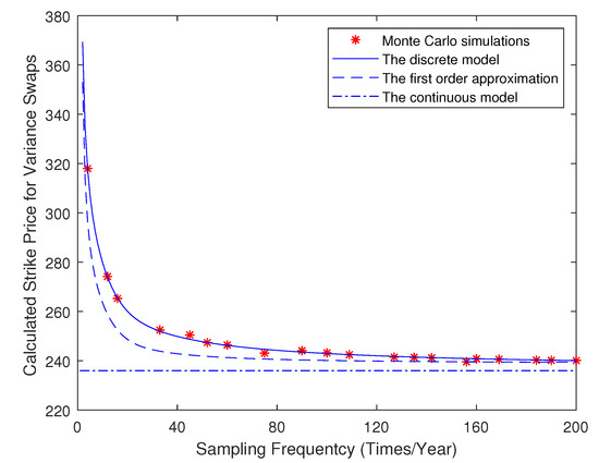
Figure 1. A comparison of fair strike prices based on the closed-solution, Monte Carlo simulations, the first-order approximation and the continuous model.

In particular, compared with the semi-solution in Cao [24,26], there is no need to adjust the parameters for our closed-form solution. In the mean time, with the increase of sampling frequency, the price curve of the closed-form solution and the approximate solution is closer and closer, eventually converge to the continuous case. Specifically, we select the prices corresponding to the above curve under different sampling frequencies, and put them together with some Monte Carlo simulation results in Table 1. According to the data in Table 1, when the sampling frequency $N=4$, the error between the closed-form solution and the approximate solution is 21.31. When the sampling frequency N reaches 200, the error is only 0.67.

Table 1. The numerical results of Monte Carlo simulations, discrete sampling, first-order approximation and continuous sampling.

Sampling Frequency	Monte Carlo	Discrete	First Order	Continuous
Quarterly (N = 4)	318.11	318.13	296.82	236.31
Monthly (N = 12)	274.24	274.02	258.91	236.31
Fortnightly(N = 16)	265.33	265.55	252.53	236.31
Weekly (N = 52)	247.43	247.48	241.80	236.31
Daily (N = 252)	240.14	240.12	239.45	236.31

4.2. Reliability of Approximate Formula

By observing the form of approximate formula, when the sampling frequency is large enough, the influence of stochastic interest rate is very small. This means that there is little difference between the results of different stochastic interest rates and the approximate formula in the case of large sampling. In order to verify this point, we need to compare the results of stochastic interest rates under different parameters. According to Cao [24] and Zhao [27], the long-term mean of stochastic interest rate $\eta$ has a great influence on the formula, but the mean-reverting speed h and volatility $\xi$ have little impact. Hence, to improve efficiency, we only select different long-term mean values, then take $h=1.2$ and $\xi =0.01$. Figure 2 shows that when the sampling frequency is small, there is a large difference between the variance swaps prices calculated by the long-term mean of different stochastic interest rates; However, with the increase of sampling frequency, the difference between these prices and the price of the approximate formula becomes smaller and smaller. This fact shows that the influence of stochastic interest rate is indeed very small when the sampling frequency is large enough. What’s more, when the sampling frequency reaches 150, the maximum error of the approximate formula does not exceed 0.8, which means that the approximate formula proposed in this paper is reliable.

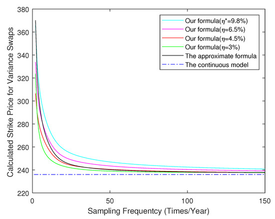
Figure 2. The values of variance swaps with different $\eta$ in our hybrid model.

5. Conclusions

In this paper, we studied the problem of pricing log-return variance swaps under the CIR–Heston hybrid model. Compared with Cao’s work, the contribution of our work is to propose a more concise approach from the perspective of stochastic analysis. There is no need to solve complex PDEs, and we obtained a closed-form solution instead of a semi-closed solution. In the mean time, considering the influence of sampling frequency on the pricing formula, we further extend the closed-form solution to an approximate formula. The advantage of the approximate solution is a simpler form and reliable in the case of large sampling. Some numerical simulation shows that our closed-form solution matches well with the results of MC simulation. By comparing the price curves of the closed-form solution and the approximate solution, we conclude that the error become smaller and smaller with the increase of sampling frequency. Moreover, in the case of large samples, the error between the closed-form solution determined from different stochastic interest rates and the approximate solution is quite little. Therefore, we have reason to confirm that the influence of stochastic interest rate on the pricing formula does decrease with the increase of sampling frequency and our approximate formula is reliable.

Finally, it should be noted that our pricing approach is general. It also can be extended to other stochastic interest rate and stochastic volatility models, such as the Heston–Hull–White hybrid model. However, when the model becomes a full coefficient correlation, how to obtain the pricing formula by the method proposed in this paper is a problem worthy of study in the future.

References

- Carr, P.; Lee, R. Volatility derivatives. Annu. Rev. Financ. Econ. 2009, 1, 319–339. [Google Scholar] [CrossRef] [Green Version]
- Grünbichler, A.; Longstaff, F.A. Valuing futures and options on volatility. J. Bank. Financ. 1996, 20, 985–1001. [Google Scholar] [CrossRef]
- Howison, S.; Rafailidis, A.; Rasmussen, H. On the pricing and hedging of volatility derivatives. Appl. Math. Financ. 2004, 11, 317–346. [Google Scholar] [CrossRef] [Green Version]
- Heston, S.; Nandi, S. Derivatives on Volatility: Some Simple Solutions Based on Observables. SSRN Electron. J. 2000. [Google Scholar] [CrossRef] [Green Version]
- Elliott, R.J.; Siu, T.K.; Chan, L. Pricing volatility swaps under Heston’s stochastic volatility model with regime switching. Appl. Math. Financ. 2007, 14, 41–62. [Google Scholar] [CrossRef]
- Swishchuk, A. Modeling and pricing of variance swaps for stochastic volatilities with delay. WILMOTT Mag. 2005, 19, 63–73. [Google Scholar]
- Swishchuk, A. Modeling and pricing of variance swaps for multi-factor stochastic volatilities with delay. Can. Appl. Math. Q. 2006, 14, 439–467. [Google Scholar]
- Habtemicael, S.; SenGupta, I. Pricing variance and volatility swaps for Barndorff-Nielsen and Shephard process driven financial markets. Int. J. Financ. Eng. 2016, 3, 1650027. [Google Scholar] [CrossRef]
- Issaka, A.; SenGupta, I. Analysis of variance based instruments for Ornstein-Uhlenbeck type models: Swap and price index. Ann. Financ. 2017, 13, 401–434. [Google Scholar] [CrossRef]
- SenGupta, I.; Wilson, W.; Nganje, W. Barndorff-Nielsen and Shephard model: Oil hedging with variance swap and option. Math. Financ. Econ. 2019, 13, 209–226. [Google Scholar] [CrossRef]
- Jarrow, R.; Kchia, Y.; Larsson, M.; Protter, P. Discretely sampled variance and volatility swaps versus their continuous approximations. Financ. Stoch. 2013, 17, 305–324. [Google Scholar] [CrossRef] [Green Version]
- Farnoosh, R.; Sobhani, A.; Rezazadeh, H.; Beheshti, M.H. Numerical method for discrete double barrier option pricing with time-dependent parameters. Comput. Math. Appl. 2015, 70, 2006–2013. [Google Scholar] [CrossRef]
- Farnoosh, R.; Sobhani, A.; Beheshti, M.H. Efficient and fast numerical method for pricing discrete double barrier option by projection method. Comput. Math. Appl. 2017, 73, 1539–1545. [Google Scholar] [CrossRef]
- Lian, G.; Zhu, S.P.; Elliott, R.J.; Cui, Z. Semi-analytical valuation for discrete barrier options under time-dependent lévy processes. J. Bank. Financ. 2017, 75, 167–183. [Google Scholar] [CrossRef]
- Little, T.; Pant, V. A finite-difference method for the valuation of variance swaps. J. Comput. Financ. 2001, 5, 81–101. [Google Scholar] [CrossRef]
- Heston, S.L. A closed-form solution for options with stochastic volatility with applications to bond and currency options. Rev. Financ. Stud. 1993, 6, 327–343. [Google Scholar] [CrossRef] [Green Version]
- Michael, A. Kouritzin, Explicit Heston solutions and stochastic approximation for path-dependent option pricing. Int. J. Theor. Appl. Financ. 2018, 21, 1850006. [Google Scholar]
- Zhu, S.P.; Lian, G.H. A closed-form exact solution for pricing variance swaps with stochastic volatility. Math. Financ. 2011, 21, 233–256. [Google Scholar]
- Zhu, S.P.; Lian, G.H. Analytically pricing volatility swaps under stochastic volatility. J. Comput. Appl. Math. 2015, 288, 332–340. [Google Scholar] [CrossRef]
- Zhang, L.W. A closed-form pricing formula for variance swaps with mean-reverting Gaussian volatility. ANZIAM J. 2014, 55, 362–382. [Google Scholar]
- Broadie, M.; Jain, A. The effect of jumps and discrete sampling on volatility and variance swaps. Int. J. Theor. Appl. Financ. 2008, 11, 761–797. [Google Scholar] [CrossRef]
- Liu, W.Y.; Zhu, S.P. Pricing variance swaps under the Hawkes jump-diffusion process. J. Futur. Mark. 2019, 39, 635–655. [Google Scholar] [CrossRef]
- Kim, J.H.; Yoon, J.H.; Yu, S.H. Multiscale stochastic volatility with the Hull-CWhite rate of interest. J. Futur. Mark. 2014, 34, 819–837. [Google Scholar] [CrossRef]
- Cao, J.; Lian, G.; Roslan, T.R.N. Pricing variance swaps under stochastic volatility and stochastic interest rate. Appl. Math. Comput. 2016, 277, 72–81. [Google Scholar] [CrossRef] [Green Version]
- Cox, J.C.; Ingersoll, J.E., Jr.; Ross, S.A. A theory of the term structure of interest rates. Econometrica 1985, 53, 385–407. [Google Scholar] [CrossRef]
- Cao, J.; Roslan, T.R.N.; Zhang, W. The valuation of variance swaps under stochastic volatility, stodwastic interest rate and full correlation structure. Korean Math. Soc. 2020, 57, 1167–1186. [Google Scholar]
- Han, Y.; Zhao, L. A closed-form pricing formula for variance swaps under MRG-Vasicek model. Comput. Appl. Math. 2019, 38, 142. [Google Scholar] [CrossRef]
- Xu, D.X.; Yang, B.Z.; Kang, J.H.; Huang, N.J. Variance and volatility swaps valuations with the stochastic liquidity risk. Phys. A Stat. Mech. Its Appl. 2021, 566, 125679. [Google Scholar] [CrossRef]
- He, X.J.; Zhu, S.P. How should a local regime-switching model be calibrated? J. Econom. Dyn. Control 2017, 78, 149–163. [Google Scholar] [CrossRef] [Green Version]
- He, X.J.; Zhu, S.P. On full calibration of hybrid local volatility and regime-switching models. J. Futur. Mark. 2018, 38, 586–606. [Google Scholar] [CrossRef]
- Zhu, S.P.; Lian, G.H. On the valuation of variance swaps with stochastic volatility. Appl. Math. Comput. 2012, 219, 1654–1669. [Google Scholar] [CrossRef]
- Bernard, C.; Cui, Z. Prices and asymptotics for discrete variance swaps. Appl. Math. Financ. 2014, 21, 140–173. [Google Scholar] [CrossRef] [Green Version]
- Zhu, S.P.; Lian, G.H. Pricing forward-start variance swaps with stochastic volatility. Appl. Math. Comput. 2015, 250, 920–933. [Google Scholar] [CrossRef]
- Cao, J.P.; Fang, Y.B. An analytical approach for variance swaps with an Ornstein-Uhlenbeck process. Aust. N. Z. Ind. Appl. Math. J. 2017, 59, 83–102. [Google Scholar]
- Sanae, R. Analytically pricing variance swaps in commodity derivative markets under stochastic convenience yields. Commun. Math. Sci. 2021, 19, 111–146. [Google Scholar]
- Larissa, B.; Maran, R.M.; Ioan, B.; Anca, N.; Mircea-Iosif, R.; Horia, T.; Gheorghe, F.; Ema Speranta, M.; Dan, M.I. Adjusted Net Savings of CEE and Baltic Nations in the Context of Sustainable Economic Growth: A Panel Data Analysis. Risk Financ. Manag. 2020, 13, 234. [Google Scholar] [CrossRef]
- Brigo, D.; Mercurio, F. Interest Rate Models-Theory and Practice: With Smile, Inflation and Credit; Springer Science and Business Media: Berlin/Heidelberg, Germany, 2007. [Google Scholar]
Publisher’s Note: MDPI stays neutral with regard to jurisdictional claims in published maps and institutional affiliations. |
© 2021 by the authors. Licensee MDPI, Basel, Switzerland. This article is an open access article distributed under the terms and conditions of the Creative Commons Attribution (CC BY) license (https://creativecommons.org/licenses/by/4.0/).