Weak Approximations of the Wright–Fisher Process

Abstract

In this paper, we construct first- and second-order weak split-step approximations for the solutions of the Wright–Fisher equation. The discretization schemes use the generation of, respectively, two- and three-valued random variables at each discretization step. The accuracy of constructed approximations is illustrated by several simulation examples.

1. Introduction

We are interested in weak first- and second-order approximations for the Wright–Fisher equation

$$X_t^x=x+{\int }_0^t(a-b{X}_s^x)ds+\sigma {\int }_0^t\sqrt{X_s^x(1-X_s^x)}d{B}_s,x\in [0,1],$$

(1)

with parameters $0\le a\le b$ and $\sigma >0$. The Wright–Fisher (WF) process (a solution of Equation (1)) is well defined in $[0,1]$ and models the gene frequencies in a population. The main problem in developing numerical methods for “square-root” diffusions is that the diffusion coefficient has unbounded derivatives near “singular” points (in our case, 0 and 1), and therefore standard methods (see, e.g., Milstein and Tretyakov [1]) are not applicable; typically, discretization schemes involving (explicitly or implicitly) the derivatives of the coefficients usually lose their accuracy near singular points, especially for large $\sigma$.

Alfonsi [2] (Chap. 6) constructed a weak second-order approximation of the WF process by using its connection with the Cox–Ingersoll–Ross (CIR) [3] process and the earlier constructed approximations of the latter (Alfonsi [4]). The main result of this paper is a direct construction of first- and second-order weak split-step approximations of the WF processes by discrete random variables. We believe that in comparison with the numerical scheme of Alfonsi [2] (Prop. 6.1.13, Algs. 6.1 and 6.2), our algorithm is much simpler and easier to implement. In our construction, we follow some ideas of Lileika and Mackevičius [5,6]. However, we had to overcome a serious additional challenge (in comparison with CIR or CKLS processes): two “singular” points, 0 and 1, of the diffusion coefficient make it essentially more difficult to ensure that the approximations take values in $[0,1]$ (instead of $[0,+\infty )$ as in [5,6]).

The paper is organized as follows. In Section 2, we recall some definitions and results. In Section 3 and Section 4, we construct first- and second-order approximations for the WF equation by two- and three-valued discrete random variables, respectively. The main results of these sections are presented as Theorems 4 and 5. We illustrate the accuracy of our approximations by several simulation examples. In Section 5, we prove an auxiliary result on the smoothness of solutions of the corresponding backward Kolmogorov PDE equation. Tedious technical calculations have been performed using Maple and Python.

2. Preliminaries

In this section, we give some known definitions adapted to our context of the WF process defined by Equation (1).

Having a fixed time interval $[0,T]$, consider an equidistant time discretization ${\Delta }^h=$$\{ih,i=0,1,\dots ,[T/h],h\in (0,T\left]\right\}$, where $\left[a\right]$ is the integer part of a. By a discretization scheme (or approximation) of Equation (1) we mean any family of discrete-time homogeneous Markov chains ${\widehat{X}}^h=\left\{{\widehat{X}}^h(x,t),x\in [0,1],t\in {\Delta }^h\right\}$ in [0, 1] with initial values ${\widehat{X}}^h(x,0)=x$ and one-step transition probabilities $p^h(x,\mathrm{d}z)$, $x\in [0,1]$. For convenience, we only consider steps $h=T/n$, $n\in \mathbb{N}$. For brevity, we sometimes write ${\widehat{X}}_t^x$ or $\widehat{X}(x,t)$ instead of ${\widehat{X}}^h(x,t)$. Note that because of the Markovity, a one-step approximation ${\widehat{X}}_h^x$ of the scheme completely defines the distribution of the whole discretization scheme ${\widehat{X}}_t^x$, so that we only need to construct the former. Therefore, we will abbreviate one-step approximations as approximations. As usual, $\mathbb{N}$ and $\mathbb{R}$ are the sets of natural and real numbers, $\overline{\mathbb{N}}:=\mathbb{N}\cup \left\{0\right\}$, and ${\mathbb{R}}_{+}:=[0,\infty )$.

We will write $g(x,h)=O\left(h^n\right)$ if, for some $C>0$ and $h_0>0,$

$$\begin{array}{c}\hfill \left|g(x,h)\right|\le C{h}^n,x\in [0,1],0<h\le h_0.\end{array}$$

Definition 1

(c.f. [4], Def. 1.3, [6], Def. 1). A discretization scheme ${\widehat{X}}^h$ is a weak νth-order approximation for the solution $\left(X_t^x,t\in [0,T]\right)$ of Equation (1) if for every $f\in C^{\infty }[0,1]$,

$$\begin{array}{c}\hfill \left|\mathbb{E}f\left(X_T^x\right)-\mathbb{E}f\left({\widehat{X}}_T^x\right)\right|=O\left(h^{\nu }\right).\end{array}$$

Definition 2

(c.f. [4], Def. 1.8, [6], Defs. 2, 3). The νth-order remainder of a discretization scheme ${\widehat{X}}_t^x$ for $X_t^x$ is the operator $R_v^h:C^{\infty }[0,1]\to C[0,1]$ defined by

$$\begin{array}{c}\hfill R_{\nu }^{h}f\left(x\right):=\mathbb{E}f\left({\widehat{X}}_h^x\right)-\left[f\left(x\right)+\sum _{k=1}^{\nu }\frac{A^{k}f\left(x\right)}{k!}{h}^k\right],x\in [0,1],h>0,\end{array}$$

where A is the generator of $X_t^x$,

$$Af\left(x\right)=(a-bx)f^{\prime }\left(x\right)+\frac{1}{2}{\sigma }^{2}x(1-x)f^{\prime \prime }\left(x\right).$$

A discretization scheme ${\widehat{X}}_t^x$ is a potential νth-order weak approximation of Equation (1) if

$$\begin{array}{c}\hfill R_{\nu }^{h}f\left(x\right)=O\left(h^{\nu +1}\right)\end{array}$$

for all $f\in C^{\infty }[0,1]$ and $x\in [0,1]$.

The following two theorems ensure that a potential $\nu$th-order weak approximation is in fact a $\nu$th-order weak approximation (in the sense of Definition 1). Note that the requirement of uniformly bounded moments (see, e.g., [4]) is obviously satisfied by our approximations since they take values in [0, 1].

Theorem 1

(see Theorem 1.19 of [4]). Let ${\widehat{X}}^h$ be a discretization scheme with transition probabilities $p^h(x,\mathrm{d}z)$ on $[0,1]$ that starts from ${\widehat{X}}_0^x=x\in [0,1]$. We assume that

1.

the scheme is a potential weak νth-order discretization scheme for the operator A.

2.

$f\in C^{\infty }[0,1]$ is a function such that $u(t,x)=\mathbb{E}f\left(X_{T-t}^x\right)$ defined on $[0,T]\times [0,1]$ solves ${\partial }_{t}u(t,x)=-Au(t,x)$ for $(t,x)\in [0,T]\times [0,1]$.

Then $|\mathbb{E}f\left({\widehat{X}}_T^x\right)-\mathbb{E}f\left(X_T^x\right)|=O\left(h^{\nu }\right)$.

Theorem 2

(see Theorem 6.1.12 of [2]). Let $f\in C^{\infty }[0,1]$. Then

$$\tilde{u}(t,x):=\mathbb{E}f\left(X_t^x\right),(t,x)\in {\mathbb{R}}_{+}\times [0,1],$$

is a $C^{\infty }$ function that solves

$$\begin{array}{c}\hfill {\partial }_t\tilde{u}(t,x)=A\tilde{u}(t,x).\end{array}$$

(2)

We split Equation (1) into the deterministic part

$$\begin{array}{c}\hfill \mathrm{d}{D}_t^x=\left(a-b{D}_t^x\right)\mathrm{d}t,D_0^x=x\in [0,1],\end{array}$$

(3)

and the stochastic part

$$\begin{array}{c}\hfill \mathrm{d}{S}_t^x=\sigma \sqrt{S_t^x(1-S_t^x)}\mathrm{d}{B}_t,S_0^x=x\in [0,1].\end{array}$$

(4)

The solution of the deterministic part is positive for all $(x,t)\in [0,1]\times (0,T]$, namely:

$$\begin{array}{c}\hfill D_t^x=D(x,t)=\left\{\begin{array}{cc}x{\mathrm{e}}^{-bt}+\frac{a}{b}\left(1-{\mathrm{e}}^{-bt}\right),\hfill & 0\le a\le b\ne 0,\hfill \\ x,\hfill & a=b=0.\hfill \end{array}\right.\end{array}$$

(5)

The solution of the stochastic part is not explicitly known. However, suppose that ${\widehat{S}}_t^x$ is a discretization scheme for the stochastic part. We define the first-order composition ${\widehat{X}}_t^x$ of the latter with the solution of the deterministic part as a Markov chain that has the transition probability in one step equal to the distribution of the random variable

$$\begin{array}{c}\hfill {\widehat{X}}^h(x,h):=D(\widehat{S}(x,h),h).\end{array}$$

(6)

Similarly, the second-order composition is defined by

$$\begin{array}{c}\hfill {\widehat{X}}^h(x,h):=D\left(\widehat{S}\left(D\left(x,\frac{h}{2}\right),h\right),\frac{h}{2}\right).\end{array}$$

(7)

Theorem 3

(see [4], Thm. 1.17). Let ${\widehat{S}}_t^x$ be a potential first- or second-order approximation of the stochastic part of the WF equation. Then, compositions (6) and (7) define, respectively, a first- or second-order approximation ${\widehat{X}}_t^x$ of the WF Equation (1).

From this theorem, it follows that to construct a first- or second-order weak approximation, we only need to construct a first- or second-order approximation of the stochastic part, respectively.

Remark 1.

For various applications, we may be interested in similar processes with values in $[\alpha ,\beta ]$ satisfying the equation

$$\mathrm{d}{\tilde{X}}_t=(\tilde{a}-b{\tilde{X}}_t)\mathrm{d}t+\sigma \sqrt{({\tilde{X}}_t-\alpha )(\beta -{\tilde{X}}_t)}\mathrm{d}{B}_t,{\tilde{X}}_0\in [\alpha ,\beta ],$$

(8)

which is well defined when $b\alpha \le \tilde{a}\le b\beta$. A popular choice is the Jacobi process with $\alpha =-1$ and $\beta =1$. Process (8) can be obtained from the WF process by the affine transformation ${\tilde{X}}_t=\alpha +(\beta -\alpha )X_t$$(\tilde{a}=a(\beta -\alpha ))$. Clearly, by the same transformation we can get weak approximations for (8) from weak approximations for the WF process.

3. First-Order Weak Approximation of Wright–Fisher Equation

3.1. Approximation of the Stochastic Part

Let us construct an approximation for the stochastic part of the WF equation, that is, the solution $S_t^x$ of Equation (1) with $a=b=0$. A two-valued discrete random variable ${\widehat{S}}_h^x$ taking values $x_1,x_2\in [0,1]$ with probabilities $p_1,p_2$ is a first-order weak approximation if (see [5] and references therein)

$$\begin{array}{cc}\hfill p_1+p_2& =1,\hfill \end{array}$$

(9)

$$\begin{array}{cc}\hfill \mathbb{E}{\widehat{S}}_h^x=x_1{p}_1+x_2{p}_2& =m_1:=\mathbb{E}{S}_h^x=x,\hfill \end{array}$$

(10)

$$\begin{array}{cc}\hfill \mathbb{E}{\left({\widehat{S}}_h^x\right)}^2=x_1^2{p}_1+x_2^2{p}_2& =m_2+O\left(h^2\right),\hfill \end{array}$$

(11)

$$\begin{array}{cc}\hfill \mathbb{E}{({\widehat{S}}_h^x-x)}^3={(x_1-x)}^3{p}_1+{(x_2-x)}^3{p}_2& =O\left(h^2\right),\hfill \end{array}$$

(12)

$$\begin{array}{cc}\hfill \mathbb{E}{({\widehat{S}}_h^x-x)}^4={(x_1-x)}^4{p}_1+{(x_2-x)}^4{p}_2& =O\left(h^2\right),\hfill \end{array}$$

(13)

where the second moment $m_2=\mathbb{E}{\left(S_h^x\right)}^2$ can be calculated by Lemma 6 with $a=b=0$:

$$\begin{array}{cc}\hfill m_2& =m_2(x,h)=x^2{e}^{-{\sigma }^{2}h}+x(1-e^{-{\sigma }^{2}h})\hfill \end{array}$$

(14)

$$\begin{array}{cc}\hfill & =x^2+x(1-x){\sigma }^{2}h+O\left(h^2\right),x\in [0,1].\hfill \end{array}$$

(15)

One of the solutions to the equation system (9)–(11) is (see [5])

$$\begin{array}{cc}\hfill x_{1,2}& =\frac{m_2}{m_1}\mp \sqrt{\frac{m_2(m_2-m_1^2)}{m_1^2}},\hfill \\ \hfill p_{1,2}& =\frac{x}{2x_{1,2}}.\hfill \end{array}$$

Therefore, in our case, we get

$$\begin{array}{cc}\hfill x_{1,2}& =x{e}^{-{\sigma }^{2}h}+1-e^{-{\sigma }^{2}h}\hfill \\ \hfill & \mp \sqrt{\frac{x{e}^{-{\sigma }^{2}h}+(1-e^{-{\sigma }^{2}h})}{x}\left(x^2{e}^{-{\sigma }^{2}h}+x(1-e^{-{\sigma }^{2}h})-x^2\right)}\hfill \end{array}$$

(16)

$$\begin{array}{cc}\hfill & =x{e}^{-{\sigma }^{2}h}+1-e^{-{\sigma }^{2}h}\mp \sqrt{(x{e}^{-{\sigma }^{2}h}+1-e^{-{\sigma }^{2}h})(1-x)(1-e^{-{\sigma }^{2}h})}.\hfill \end{array}$$

(17)

Since $1-e^{-{\sigma }^{2}h}={\sigma }^{2}h+O\left(h^2\right)$, to simplify the expressions, we may try to replace $1-e^{-{\sigma }^{2}h}$ by ${\sigma }^{2}h$ and, instead of (17), use

$$\begin{array}{cc}\hfill x_{1,2}=x_{1,2}(x,h)& =x(1-{\sigma }^{2}h)+{\sigma }^{2}h\mp \sqrt{(x(1-{\sigma }^{2}h)+{\sigma }^{2}h)(1-x){\sigma }^{2}h}\hfill \\ \hfill & =x+(1-x){\sigma }^{2}h\mp \sqrt{(x+(1-x){\sigma }^{2}h)(1-x){\sigma }^{2}h}.\hfill \end{array}$$

(18)

In Lemma 1, we will check that after this replacement, $x_{1,2}$ and $p_{1,2}$ still satisfy (9)–(13). Unfortunately, for the values of x near 1, the values of $x_2$ are slightly greater than 1 (as well as those defined by (17)), which is unacceptable. We overcome this problem by using the symmetry of the solution of the stochastic part with respect to the point $\frac{1}{2}$; to be precise, $S_t^x\stackrel{d}{=}1-S_t^{1-x}$ for all $x\in [0,1]$ ($\stackrel{d}{=}$ means equality in distribution). Therefore, in the interval $[0,1/2],$ we can use the values $x_{1,2}$ defined by (18), whereas in the interval $(1/2,1],$ we use the values corresponding to the process $1-S_t^{1-x}$, that is,

$$\begin{array}{cc}\hfill {\tilde{x}}_{1,2}={\tilde{x}}_{1,2}(x,h)& :=1-x_{1,2}(1-x,h)\hfill \\ \hfill & =x-x{\sigma }^{2}h\pm \sqrt{(1-x+x{\sigma }^{2}h)x{\sigma }^{2}h}\hfill \end{array}$$

(19)

with probabilities ${\tilde{p}}_{1,2}=\frac{1-x}{2x_{1,2}(1-x,h)}$. Thus, we obtain the acceptable (i.e., with values in [0, 1]) approximation ${\widehat{S}}_h^x$ taking the values

$$\begin{array}{cc}\hfill {\widehat{x}}_{1,2}& :=\left\{\begin{array}{cc}{x}_{1,2}(x,h)\mathrm{with} \mathrm{probabilities}{p}_{1,2}=\frac{x}{2x_{1,2}(x,h)},\hfill & x\in [0,1/2],\hfill \\ 1-x_{1,2}(1-x,h)\mathrm{with} \mathrm{probabilities}{p}_{1,2}=\frac{1-x}{2x_{1,2}(1-x,h)},\hfill & x\in (1/2,1].\hfill \end{array}\right.\hfill \end{array}$$

(20)

Lemma 1.

The values ${\widehat{x}}_{1,2}$ defined by (20) satisfy conditions (9)–(13), and ${\widehat{x}}_{1,2}\in [0,1]$.

Proof. 

We first check that $x_{1,2}$ defined by (18) obtain values from the interval [0, 1] when $x\in [0,1/2]$ and h is sufficiently small ($0<h\le h_0$ with $h_0>0$ independent from x):

$$\begin{array}{cc}\hfill x_1& =x+(1-x){\sigma }^{2}h-\sqrt{(x+(1-x){\sigma }^{2}h)(1-x){\sigma }^{2}h}\ge 0\hfill \\ \hfill & \iff x+(1-x){\sigma }^{2}h\ge \sqrt{(x+(1-x){\sigma }^{2}h)(1-x){\sigma }^{2}h}\hfill \\ \hfill & \iff x+(1-x){\sigma }^{2}h\ge (1-x){\sigma }^{2}h\hfill \\ \hfill & \iff x\ge 0;\hfill \\ \hfill x_2& =x+(1-x){\sigma }^{2}h+\sqrt{(x+(1-x){\sigma }^{2}h)(1-x){\sigma }^{2}h}\le 1\hfill \\ \hfill & \iff \sqrt{(x+(1-x){\sigma }^{2}h)(1-x){\sigma }^{2}h}\le (1-x)(1-{\sigma }^{2}h)\hfill \\ \hfill & \iff x{\sigma }^{2}h+(1-x){\left({\sigma }^{2}h\right)}^2\le (1-x){(1-{\sigma }^{2}h)}^2\hfill \\ \hfill & \iff x{\sigma }^{2}h+(1-x){\left({\sigma }^{2}h\right)}^2\le (1-x)(1-2{\sigma }^{2}h+{\left({\sigma }^{2}h\right)}^2)\hfill \\ \hfill & \iff x{\sigma }^{2}h\le (1-x)(1-2{\sigma }^{2}h)\hfill \\ \hfill & \iff x{\sigma }^{2}h+1-x-2{\sigma }^{2}h\ge 0.\hfill \end{array}$$

If $x\in [0,1/2]$, then

$$x{\sigma }^{2}h+1-x-2{\sigma }^{2}h\ge 1/2-2{\sigma }^{2}h\ge 0,\mathrm{where} 0<h\le h_0:=\frac{1}{4{\sigma }^2}.$$

(21)

Thus $0\le x_1<x_2\le 1$ for $x\in [0,1/2]$ and $0<h\le h_0=1/4{\sigma }^2$. So, if $x\in (1/2,1]$, then $1-x\in [0,1/2)$, and according to (19), instead of $x_{1,2}$, we can take ${\tilde{x}}_{1,2}=1-x_{1,2}(1-x,h)$ for $0<h\le h_0$. Thus, as we have just checked, we have $0\le x_{1,2}(1-x,h)\le 1$, that is, $0\le {\tilde{x}}_{1,2}\le 1$ for $x\in (1/2,1]$ and $0<h\le h_0$.

Now we check conditions (9)–(13) for $x_{1,2}$:

$$\begin{array}{cc}\hfill p_1+p_2& =\frac{x}{2x_1}+\frac{x}{2x_2}\hfill \\ \hfill & =\frac{2x(x+(1-x){\sigma }^{2}h)}{2((x^2+2x(1-x){\sigma }^{2}h+{(1-x)}^2{\left({\sigma }^{2}h\right)}^2-(x(1-x){\sigma }^{2}h+{(1-x)}^2{\left({\sigma }^{2}h\right)}^2)}\hfill \\ \hfill & =\frac{2x(x+(1-x){\sigma }^{2}h)}{2((x^2+x(1-x){\sigma }^{2}h)}=1;\hfill \\ \hfill x_1{p}_1+x_2{p}_2& =x_1\frac{x}{2x_1}+x_2\frac{x}{2x_2}=x,\hfill \\ \hfill x_1^2{p}_1+x_2^2{p}_2& =x_1^2\frac{x}{2x_1}+x_2^2\frac{x}{2x_2}=\frac{x}{2}(x_1+x_2)\hfill \\ \hfill & =\frac{x}{2}·2(x+(1-x){\sigma }^{2}h)=x^2+x(1-x){\sigma }^{2}h\hfill \\ \hfill & =m_2+O\left(h^2\right);\hfill \\ \hfill {(x_1-x)}^3{p}_1& +{(x_2-x)}^3{p}_2=2x{(1-x)}^2{\left({\sigma }^{2}h\right)}^2=O\left(h^2\right),\hfill \\ \hfill {(x_1-x)}^4{p}_1& +{(x_2-x)}^4{p}_2=x{(1-x)}^2(x+4(1-x){\sigma }^{2}h){\left({\sigma }^{2}h\right)}^2=O\left(h^2\right).\hfill \end{array}$$

The last two equalities were obtained by using the Python SymPy package. The conditions for ${\tilde{x}}_{1,2}$ follow automatically from the symmetry. □

For the initial Equation (1) we obtain an approximation ${\widehat{X}}_h^x$ by the “split-step” procedure defined by (6):

$${\widehat{X}}_h^x:={\widehat{S}}_h^x{e}^{-bh}+\frac{a}{b}(1-e^{-bh}).$$

(22)

Now we can state our first main result.

Theorem 4.

Let ${\widehat{X}}_t^x$ be the discretization scheme defined by one-step approximation (22). Then, ${\widehat{X}}_t^x$ is a first-order weak approximation of Equation (1) for functions $f\in C^{\infty }[0,1]$.

3.2. Algorithm

In this section, we provide an algorithm for calculating ${\widehat{X}}_{(i+1)h}$ given ${\widehat{X}}_{ih}=x$ at each simulation step i:

1.

Draw a uniform random variable U from the interval [0, 1].

2.

If $x\le \frac{1}{2}$, then

–

calculate $x_1,x_2$ according to (18),

2.

else

–

calculate $x_1,x_2$ according to (18) with $x:=1-x$,

–

$x_{1,2}:=1-x_{1,2}$.

3.

Calculate $p_{1,2}:=\frac{x}{2x_{1,2}(x,h)}$.

4.

If $U<p_1$, then $\widehat{S}:=x_1$ else $\widehat{S}:=x_2$.

5.

Calculate (see (6) and (22))

$$\begin{array}{c}\hfill {\widehat{X}}_{(i+1)h}=D\left(\widehat{S},h\right)=\widehat{S}{e}^{-bh}+\frac{a}{b}(1-e^{-bh}).\end{array}$$

3.3. Simulation Examples

We illustrate our approximation for the test functions $f\left(x\right)=x^5$ and $f\left(x\right)={\mathrm{e}}^{-x}$. Since we do not explicitly know the moments $\mathbb{E}{\mathrm{e}}^{-X_t^x}$, we use the approximate equality ${\mathrm{e}}^{-x}\approx 1-x+\frac{x^2}{2}-\frac{x^3}{6}+\frac{x^4}{24}-\frac{x^5}{120}$. We have chosen the parameters of the WF equation so that the fifth moment of $X_t^x$ is nonmonotonic as a function of t to see how the approximated fifth moment “follows” the bends of the true one as t varies. In Figure 1, Figure 2 and Figure 3, we compare $\mathbb{E}f\left({\widehat{X}}_t^x\right)$ and $\mathbb{E}f\left(X_t^x\right)$ as functions of t (left plots) and as functions of a discretization step h (right plots) in terms of the relative error $|1-\frac{\mathbb{E}f\left({\widehat{X}}_t^x\right)}{\mathbb{E}f\left(X_t^x\right)}|$. As expected, the approximations agree with exact values pretty well. Note an impressive match between the approximated and true values of $\mathbb{E}{\mathrm{e}}^{-X_t^x}$ in Figure 3 even for rather large discretization step h.

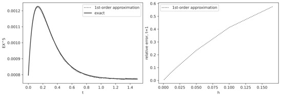
Figure 1. Comparison of $\mathbb{E}f\left({\widehat{X}}_t^x\right)$ and $\mathbb{E}f\left(X_t^x\right)$ as functions of t and h for $f\left(x\right)=x^5$: $x=0.24$, ${\sigma }^2=0.6,a=0.8,b=5$, the number of iterations $N=1,000,000$. Left: $h=0.001$; Right: the relative error at $t=1.$

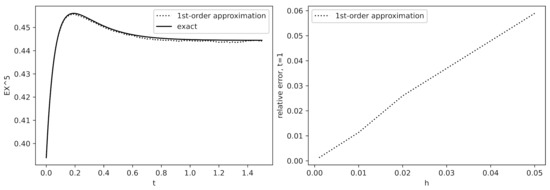
Figure 2. Comparison of $\mathbb{E}f\left({\widehat{X}}_t^x\right)$ and $\mathbb{E}f\left(X_t^x\right)$ as functions of t and h for $f\left(x\right)=x^5$: $x=0.83$, ${\sigma }^2=2,a=4,b=5,N=1,000,000$. Left: $h=0.001$; Right: the relative error at $t=1.$

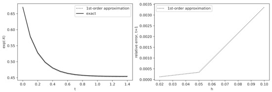
Figure 3. Comparison of $\mathbb{E}f\left({\widehat{X}}_t^x\right)$ and $\mathbb{E}f\left(X_t^x\right)$ as functions of t and h for $f\left(x\right)={\mathrm{e}}^{-x}$: $x=0.4$, ${\sigma }^2=1.6,a=4,b=5,N=\mathrm{100,000}$. Left: $h=0.1$; Right: the relative error at $t=1.$

4. Second-Order Weak Approximation of Wright–Fisher Equation

4.1. Approximation of the Stochastic Part

Let ${\widehat{S}}_h^x$ be any discretization scheme. Applying Taylor’s formula to $f\in C^{\infty }[0,1]$, we have

$$\begin{array}{cc}\hfill \mathbb{E}f\left({\widehat{S}}_h^x\right)& =f\left(x\right)+f^{\prime }\left(x\right)\mathbb{E}\left({\widehat{S}}_h^x-x\right)+\frac{f^{\prime \prime }\left(x\right)}{2}\mathbb{E}{\left({\widehat{S}}_h^x-x\right)}^2+\frac{f^{\prime \prime \prime }\left(x\right)}{6}\mathbb{E}{\left({\widehat{S}}_h^x-x\right)}^3\hfill \\ \hfill & +\frac{f^{\left(4\right)}\left(x\right)}{4!}\mathbb{E}{\left({\widehat{S}}_h^x-x\right)}^4+\frac{f^{\left(5\right)}\left(x\right)}{5!}\mathbb{E}{\left({\widehat{S}}_h^x-x\right)}^5\hfill \\ \hfill & +\frac{1}{5!}\mathbb{E}{\int }_x^{{\widehat{S}}_h^x}{f}^{\left(6\right)}\left(s\right){\left({\widehat{S}}_h^x-s\right)}^5\mathrm{d}s.\hfill \end{array}$$

The generator $A_0$ and its square of the stochastic part are

$$\begin{array}{cc}\hfill A_{0}f\left(x\right)& =\frac{1}{2}{\sigma }^{2}x(1-x)f^{\prime \prime }\left(x\right),\hfill \\ \hfill A_0^{2}f\left(x\right)& =-\frac{1}{2}{\sigma }^{4}x(1-x)f^{\prime \prime }\left(x\right)+\frac{1}{2}{\sigma }^{4}x(1-x)(1-2x)f^{\prime \prime \prime }\left(x\right)\hfill \\ \hfill & +\frac{1}{4}{\sigma }^4{x}^2{(1-x)}^2{f}^{\left(4\right)}\left(x\right).\hfill \end{array}$$

Thus, the second-order remainder of the discretization scheme ${\widehat{S}}_h^x$ is

$$\begin{array}{cc}\hfill R_2^{h}f\left(x\right)& =\mathbb{E}f\left({\widehat{S}}_h^x\right)-\left[f\left(x\right)+A_{0}f\left(x\right)h+A_0^{2}f\left(x\right)\frac{h^2}{2}\right]\hfill \\ \hfill & =f^{\prime }\left(x\right)\mathbb{E}\left({\widehat{S}}_h^x-x\right)\hfill \\ \hfill & +\frac{f^{\prime \prime }\left(x\right)}{2}\left[\mathbb{E}{\left({\widehat{S}}_h^x-x\right)}^2-{\sigma }^{2}x(1-x)h\left(1-\frac{1}{2}{\sigma }^{2}h\right)\right]\hfill \\ \hfill & +\frac{f^{\prime \prime \prime }\left(x\right)}{6}\left[\mathbb{E}{\left({\widehat{S}}_h^x-x\right)}^3-\frac{3}{2}{\sigma }^4{h}^{2}x(1-x)(1-2x)\right]\hfill \\ \hfill & +\frac{f^{\left(4\right)}\left(x\right)}{4!}\left[\mathbb{E}{\left({\widehat{S}}_h^x-x\right)}^4-3{\sigma }^4{\left(x(1-x)h\right)}^2\right]\hfill \\ \hfill & +\frac{f^{\left(5\right)}\left(x\right)}{5!}\mathbb{E}{\left({\widehat{S}}_h^x-x\right)}^5+r_2(x,h),x\ge 0,h>0,\hfill \end{array}$$

where

$$\begin{array}{cc}\hfill \left|r_2(x,h)\right|& =\frac{1}{5!}\left|\mathbb{E}{\int }_x^{{\widehat{S}}_h^x}{f}^{\left(6\right)}\left(s\right){\left({\widehat{S}}_h^x-s\right)}^5\mathrm{d}s\right|\le \frac{1}{6!}\underset{s\in [0,1]}{max}\left|f^{\left(6\right)}\left(s\right)\right|\mathbb{E}{\left({\widehat{S}}_h^x-x\right)}^6.\hfill \end{array}$$

This expression shows that ${\widehat{S}}_h^x$ is a potential second-order approximation of the stochastic part (4) if

$$\begin{array}{cc}\hfill & \mathbb{E}\left({\widehat{S}}_h^x-x\right)=O\left(h^3\right),\hfill \end{array}$$

(23)

$$\begin{array}{cc}\hfill & \mathbb{E}{\left({\widehat{S}}_h^x-x\right)}^2={\sigma }^{2}x(1-x)h\left(1-\frac{1}{2}{\sigma }^{2}h\right)+O\left(h^3\right),\hfill \end{array}$$

(24)

$$\begin{array}{cc}\hfill & \mathbb{E}{\left({\widehat{S}}_h^x-x\right)}^3=\frac{3}{2}{\sigma }^4{h}^{2}x(1-x)(1-2x)+O\left(h^3\right),\hfill \end{array}$$

(25)

$$\begin{array}{cc}\hfill & \mathbb{E}{\left({\widehat{S}}_h^x-x\right)}^4=3{\sigma }^4{\left(x(1-x)h\right)}^2+O\left(h^3\right),\hfill \end{array}$$

(26)

$$\begin{array}{cc}\hfill & \mathbb{E}{\left({\widehat{S}}_h^x-x\right)}^5=O\left(h^3\right),\hfill \end{array}$$

(27)

$$\begin{array}{cc}\hfill & \mathbb{E}{\left({\widehat{S}}_h^x-x\right)}^6=O\left(h^3\right).\hfill \end{array}$$

(28)

Let us denote $z={\sigma }^{2}h$ for brevity. Converting the central moments of ${\widehat{S}}_h^x$ to noncentral moments, from (23)–(28) we get

$$\begin{array}{cc}\hfill \mathbb{E}{\left({\widehat{S}}_h^x\right)}^i& ={\widehat{m}}_i+O\left(h^3\right),i=1,\dots ,6,\hfill \end{array}$$

(29)

where

$$\begin{array}{cc}\hfill {\widehat{m}}_1& =x,\hfill \\ \hfill {\widehat{m}}_2& =x^2+zx(1-x)(1-\frac{1}{2}z),\hfill \\ \hfill {\widehat{m}}_3& =x^3+\frac{3}{2}x{z}^2(3x^2-4x+1)-3xz(x^2-x),\hfill \\ \hfill {\widehat{m}}_4& =x^4+9x^2{z}^2(2x^2-3x+1)-6x^{2}z(x^2-x),\hfill \\ \hfill {\widehat{m}}_5& =x^5+10x^3{z}^2(5x^2-8x+3)-10x^{3}z(x^2-x),\hfill \\ \hfill {\widehat{m}}_6& =x^6+\frac{75}{2}{x}^4{z}^2(3x^2-5x+2)-15x^{4}z(x^2-x).\hfill \end{array}$$

(30)

Our aim is to construct a potential second-order approximation for the WF equation by discrete random variables at each generation step. Therefore, we look for approximations ${\widehat{S}}_h^x$ taking three values $x_1,x_2,x_3$ from the interval $[0,1]$ with probabilities $p_1,p_2,p_3$ satisfying the following conditions:

$$\begin{array}{cc}\hfill p_1+p_2+p_3& =1,\hfill \end{array}$$

(31)

$$\begin{array}{cc}\hfill x_1^i{p}_1+x_2^i{p}_2+x_3^i{p}_3& ={\widehat{m}}_i+O\left(h^3\right),i=1,\dots ,6.\hfill \end{array}$$

(32)

In anticipation, note that when solving system (31)–(32), a serious challenge is ensuring the first equality $p_1+p_2+p_3=1$. A simple way out of this situation is relaxing the latter by the inequality

$$p_1+p_2+p_3\le 1$$

(33)

and, at the same time, allowing ${\widehat{S}}_h^x$ to take the additional trivial value 0 with probability $p_0=1-(p_1+p_2+p_3)$. Notice that this does not change Equation (32) in any way.

Solving the system

$$\begin{array}{cc}\hfill x_1^i{p}_1+x_2^i{p}_2+x_3^i{p}_3& ={\widehat{m}}_i,i=1,2,3,\hfill \end{array}$$

with respect to $x_1,x_2,x_3$, we obtain (cf. [6])

$$\begin{array}{cc}\hfill p_1& =\frac{{\widehat{m}}_1{x}_2{x}_3-{\widehat{m}}_2{x}_2-{\widehat{m}}_2{x}_3+{\widehat{m}}_3}{x_1(x_1-x_3)(x_1-x_2)},\hfill \\ \hfill p_2& =-\frac{{\widehat{m}}_1{x}_1{x}_3-{\widehat{m}}_2{x}_1-{\widehat{m}}_2{x}_3+{\widehat{m}}_3}{x_2(x_1-x_2)(x_2-x_3)},\hfill \\ \hfill p_3& =\frac{{\widehat{m}}_1{x}_1{x}_2-{\widehat{m}}_2{x}_1-{\widehat{m}}_2{x}_2+{\widehat{m}}_3}{x_3(x_2-x_3)(x_1-x_3)}.\hfill \end{array}$$

(34)

Note that, here, differently from [6], we used approximate “moments” ${\widehat{m}}_i$ instead of the true moments $m_i$. This eventually allows us to get simpler expressions because ${\widehat{m}}_i$ are polynomials in x and z.

Now we have to find $x_{1,2,3}$ that, together with $p_{1,2,3}$ defined by Equations (34), satisfy the remaining conditions

$$\begin{array}{cc}\hfill & \left\{\begin{array}{cc}{x}_1^4{p}_1+x_2^4{p}_2+x_3^4{p}_3-{\widehat{m}}_4=O\left(h^3\right),\hfill & \\ x_1^5{p}_1+x_2^5{p}_2+x_3^5{p}_3-{\widehat{m}}_5=O\left(h^3\right),\hfill & \\ x_1^6{p}_1+x_2^6{p}_2+x_3^6{p}_3-{\widehat{m}}_6=O\left(h^3\right).\hfill \end{array}\right.\hfill \end{array}$$

(35)

Motivated by the first-order approximation (20) and [6], we look for $x_{1,2,3}$ of the following form:

$$\begin{array}{cc}\hfill x_1& =x+z{A}_1(1-x)+A_{2}xz-\sqrt{\left(z\right(1-x\left)\right(Bx+Cz(1-x)\left)\right)},\hfill \end{array}$$

(36)

$$\begin{array}{cc}\hfill x_2& =x+A_{3}xz,\hfill \end{array}$$

(37)

$$\begin{array}{cc}\hfill x_3& =x+z{A}_1(1-x)+A_{2}xz+\sqrt{\left(z\right(1-x\left)\right(Bx+Cz(1-x)\left)\right)},\hfill \end{array}$$

(38)

with unknown parameters $A_1,A_2,A_3,B,C\ge 0$.

4.2. Calculation of the Parameters

Substituting (36)–(38) into the left-hand sides of (35), we have (for technical calculations, using Maple and Python)

$$\begin{array}{cc}\hfill x_1^4{p}_1+x_2^4{p}_2+x_3^4{p}_3-{\widehat{m}}_4& =[(B{A}_3+B+2A_1-2A_2-A_3-6)x^4\hfill \\ \hfill & +\left(A_3-2B-A_{3}B-4A_1+2A_2+\frac{21}{2}\right)x^3\hfill \\ \hfill & +\left(B+2A_1-\frac{9}{2}\right)x^2]z^2+O\left(h^3\right),\hfill \end{array}$$

(39)

$$\begin{array}{cc}\hfill x_1^5{p}_1+x_2^5{p}_2+x_3^5{p}_3-{\widehat{m}}_5& =[(8A_1+(4B-4)A_3+5B-8A_2-27)x^5\hfill \\ \hfill & +\left((-4B+4)A_3-10B+8A_2-16A_1+48\right)x^4\hfill \\ \hfill & +(8A_1+5B-21)x^3]z^2+O\left(h^3\right),\hfill \end{array}$$

(40)

$$\begin{array}{cc}\hfill x_1^6{p}_1+x_2^6{p}_2+x_3^6{p}_3-{\widehat{m}}_6& =[(20A_1+(10B-10)A_3+15B-20A_2-75)x^6\hfill \\ \hfill & +\left((-10B+10)A_3-30B+20A_2-40A_1+135\right)x^5\hfill \\ \hfill & +(15B+20A_1-60)x^4]z^2+O\left(h^3\right).\hfill \end{array}$$

(41)

To ensure equalities (35), we need to choose $A_1,A_2,A_3,B$ such that expressions at $z^2$ would be equal to 0. Equating the coefficients at the lowest powers of x to zero, we get the system for the parameters $A_1$ and B:

$$\begin{array}{cc}\hfill & \left\{\begin{array}{cc}B+2A_1-\frac{9}{2}\hfill & =0,\hfill \\ 8A_1+5B-21\hfill & =0,\hfill \\ 15B+20A_1-60\hfill & =0.\hfill \end{array}\right.\hfill \end{array}$$

Although the system contains three equations with respect to two unknowns, it has the solution $A_1=\frac{3}{4},B=3.$ Substituting these values back to Equations (39)–(41), we get the relation $A_3=A_2+\frac{3}{4},$ which makes all the expressions at $z^2$ vanish. Summarizing, we have that $x_{1,2,3}$ of the form (36)–(38) and $p_{1,2,3}$ defined by (34) satisfy all of Equation (32), provided that the parameters satisfy the following relations:

$$A_1=\frac{3}{4},A_2\ge 0,A_3=A_2+\frac{3}{4},B=3,C\ge 0.$$

(42)

4.3. Positivity of the Solution

Now we would like to choose the values of free parameters $A_2$ and C so that all $x_1,x_2,x_3,p_1,p_2,p_3$ are positive and $p_1+p_2+p_3\le 1$. We first consider the latter restriction.

Lemma 2.

We have $p_1+p_2+p_3\le 1$ if

$$A_2\ge \frac{{(3+2\sqrt{2})}^{\frac{1}{3}}}{4}+\frac{1}{4{(3+2\sqrt{2})}^{\frac{1}{3}}}\approx 0.58883$$

(43)

and

$$0\le C\le \frac{3(32A_2^3-6A_2-3)}{16A_2^2(16A_2^2+24A_2+9)}.$$

Proof. 

We have

$$\begin{array}{c}\hfill p_1+p_2+p_3=\frac{N}{D}\end{array}$$

with numerator

$$\begin{array}{cc}\hfill N& =64x^2+\left((192A_2+144)x^2-96x\right)z\hfill \\ \hfill & +\left((192A_2^2-64C+96A_2+108)x^2+(128C-144)x-64C+36\right)z^2\hfill \\ \hfill & +\left(48+(-96A_2+24)x^2+(96A_2-72)x\right)z^3\hfill & \hfill \end{array}$$

and denominator

$$\begin{array}{cc}\hfill D& =64x^2+\left((192A_2+144)x^2-96x\right)z\hfill \\ \hfill & +\left((192A_2^2-64C+96A_2+108)x^2+(128C-144)x-64C+36\right)z^2\hfill \\ \hfill & +\left((64A_2^3-64C{A}_2-48A_2^2-48C-36A_2+27\right)x^2\hfill \\ \hfill & +\left(128C{A}_2+96A_2^2+96C-54)x-64A_{2}C-48C+36A_2+27\right)z^3.\hfill \end{array}$$

The numerator and denominator differ only by the coefficients at $z^3$. Thus, it suffices to show that their difference $D-N$ is nonnegative, that is,

$$\begin{array}{cc}\hfill & (64A_2^3-48A_2^2+(-64C+60)A_2-48C+3)x^2\hfill \\ \hfill & +(96A_2^2+(128C-96)A_2+96C+18)x\hfill \\ \hfill & +(-64C+36)A_2-48C-21=:a_1{x}^2+a_{2}x+a_3\ge 0.\hfill \end{array}$$

(44)

Inequality (44) is satisfied for all $x\in \mathbb{R}$ if

$$\begin{array}{c}\hfill a_1>0\mathrm{and}{a}_3\ge \frac{a_2^2}{4a_1}.\end{array}$$

(45)

Solving inequality (45), we get

$$\begin{array}{c}\hfill A_2>0,C\le \frac{3(32A_2^3-6A_2-3)}{16(16A_2^2+24A_2+9)A_2^2}.\end{array}$$

Since C must be nonnegative, we obtain condition (43) for $A_2$. □

Remark 2.

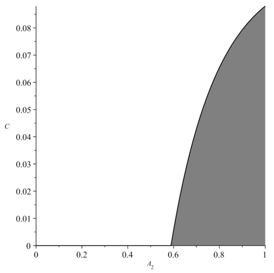
We observe that possible values of C are rather small (see Figure 4). Therefore, to simplify the expressions for $x_1,x_2,x_3$, we simply take $C=0$ and $A_2=\frac{2}{3}$.

Figure 4. Possible values of $A_2$ and $C.$

We have now arrived at the following expressions for $x_1,x_2,x_3$:

$$\begin{array}{cc}\hfill x_1& =x+\frac{3(1-x)z}{4}+\frac{2xz}{3}-\sqrt{3x(1-x)z},\hfill \end{array}$$

(46)

$$\begin{array}{cc}\hfill x_2& =x+\frac{17xz}{12},\hfill \end{array}$$

(47)

$$\begin{array}{cc}\hfill x_3& =x+\frac{3(1-x)z}{4}+\frac{2xz}{3}+\sqrt{3x(1-x)z}.\hfill \end{array}$$

(48)

However, the game is not over. At this point, we only have that $x_1,x_2,x_3$ defined by (46)–(48), together with $p_1,p_2,p_3$ defined by (34), satisfy conditions (32) and (33). From numerical calculations it appears that for “small” x, it happens that $x_1>x_2$ and thus $p_1,p_2<0.$ Moreover, on the other hand, for “not small” x and “large” h, it happens that $x_3>1$. We can see a typical situation in Figure 5 with $z={\sigma }^{2}h=\frac{1}{5}$, where for small x, $p_1$ and $p_2$ take values outside the interval $[0,1]$, whereas $x_3>1$ for x near $\frac{1}{2}$.

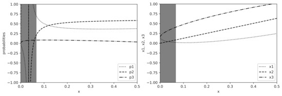
Figure 5. Graphs of $p_{1,2,3}$ (Left) and $x_{1,2,3}$ (Right) as functions of x with fixed z. Gray area shows the region where first-order approximation is used to avoid negative probabilities. Parameters: $K=\frac{1}{3},z=\frac{1}{5}$.

Due to these reasons, similarly to [4], for small x below the threshold $Kz$ (with some fixed $K>0$), we will switch to the first-order approximation (20), which behaves as a second-order one for such x. We also have to consider $z\le z_0$, where $z_0$ is to be sufficiently small to ensure that $x_3\le 1$. To be precise, for $0\le x\le Kz$, $0<z\le z_0$, we will use scheme (20), whereas for $Kz\le x\le \frac{1}{2}$, $0<z\le z_0$, we will use scheme (46)–(48) together with (34); finally, for $x\in (\frac{1}{2},1]$, we will use the symmetry $S_t^x\stackrel{d}{=}1-S_t^{1-x}$ as in the first-order approximation. The following lemmas justify such a switch for $K=\frac{1}{3}$ and $z_0=\frac{1}{6}$.

Lemma 3.

The first-order approximation (20) in the region $x\le K{\sigma }^{2}h$ (with arbitrary fixed $K>0)$ satisfies conditions (29). In other words, in this region, it behaves as a second-order approximation.

Proof. 

We prove equalities (29) in the region $x\le Kz=K{\sigma }^{2}h$, where ${\widehat{S}}_x^h$ and ${\widehat{m}}_i$, $i=1,\dots ,6,$ are defined by (20) and (30), respectively:

$$\begin{array}{cc}\hfill \mathbb{E}{\left({\widehat{S}}_h^x\right)}^2-{\widehat{m}}_2& =x_1^2{p}_1+x_2^2{p}_2-{\widehat{m}}_2\hfill \\ \hfill & =x^2+x(1-x)z-(x^2+zx(1-x)(1-\frac{1}{2}z))\hfill \\ \hfill & =\frac{1}{2}x(1-x)z^2=O\left(h^3\right),\hfill \\ \hfill \mathbb{E}{\left({\widehat{S}}_h^x\right)}^3-{\widehat{m}}_3& =x_1^3{p}_1+x_2^3{p}_2-{\widehat{m}}_3\hfill \\ \hfill & =x^3-3xz(x^2-x)+2z^2{x}^2(x-1)\hfill \\ \hfill & -(x^3+\frac{3}{2}x{z}^2(3x^2-4x+1)-3xz(x^2-x))\hfill \\ \hfill & =\frac{1}{2}x{z}^2(5x^2-8x+3)=O\left(h^3\right),\hfill \\ \hfill \mathbb{E}{\left({\widehat{S}}_h^x\right)}^4-{\widehat{m}}_4& =x_1^4{p}_1+x_2^4{p}_2-{\widehat{m}}_4=x^4-6x^{2}z(x^2-x)\hfill \\ \hfill & +x^2{z}^2(9x^2-10x+1)-4x^3{z}^3(x-1)\hfill \\ \hfill & -(x^4+9x^2{z}^2(2x^2-3x+1)-6x^{2}z(x^2-x))\hfill \\ \hfill & =x^2{z}^2(-4x^{2}z-9x^2+4xz+17x-8)=O\left(h^4\right),\hfill \\ \hfill \mathbb{E}{\left({\widehat{S}}_h^x\right)}^5-{\widehat{m}}_5& =x_1^5{p}_1+x_2^5{p}_2-{\widehat{m}}_5=x^5-10x^{3}z(x^2-x)\hfill \\ \hfill & +5x^3{z}^2(5x^2-6x+1)+4x^3{z}^3(-6x^2+7x-1)\hfill \\ \hfill & +8x^4{z}^4(x-1)\hfill \\ \hfill & -(x^5+10x^3{z}^2(5x^2-8x+3)-10x^{3}z(x^2-x))\hfill \\ \hfill & =x^3{z}^2(x^2(8z^2-24z-25)-2x(4z^2-14z-25)-4z-25)=O\left(h^5\right),\hfill \\ \hfill \mathbb{E}{\left(S_h^x\right)}^6-{\widehat{m}}_6& =x_1^6{p}_1+x_2^6{p}_2-{\widehat{m}}_6=x^6-15x^{4}z(x^2-x)\hfill \\ \hfill & +5x^4{z}^2(11x^2-14x+3)\hfill \\ \hfill & +x^3{z}^3(-85x^3+111x^1-27x+1)\hfill \\ \hfill & +12x^4{z}^4(5x^2-6x+1)-16x^5{z}^5(x-1)\hfill \\ \hfill & -(x^6+\frac{75}{2}{x}^4{z}^2(3x^2-5x+2)-15x^{4}z(x^2-x))\hfill \\ \hfill & =\frac{1}{2}{x}^3{z}^2(x-1)(-32x^2{z}^3+120x^2{z}^2-170x^{2}z\hfill \\ \hfill & -115x^2-24x{z}^2-170xz+120x-2z)=O\left(h^6\right).\square \hfill \end{array}$$

Lemma 4.

For $z\in [0,\frac{1}{6}]$ and $x\in [0,\frac{1}{2}]$, $x_1,x_2,x_3$ defined in (46)–(48) take values in the interval $[0,1]$.

Proof. 

Obviously, $x_2\in [0,1]$. Thus, we focus on $x_1$ and $x_3$. Since $x_1\le x_3$, it suffices to prove that $x_1\ge 0$ and $x_3\le 1$.

The condition $x_1\ge 0$ is equivalent to the inequality

$${\left(x+\frac{3(1-x)z}{4}+\frac{2xz}{3}\right)}^2-3x(1-x)z\ge 0.$$

By denoting $y=1-x>0$, this becomes

$$\begin{array}{cc}{\left(x+\frac{3yz}{4}+\frac{2xz}{3}\right)}^2-3xyz\hfill & \\ & \hfill =x^2+\frac{9}{16}{y}^2{z}^2+\frac{4}{9}{x}^2{z}^2-\frac{3}{2}xyz+\frac{4}{3}{x}^{2}z+xy{z}^2\ge 0.\end{array}$$

We will prove the stronger inequality

$$x^2+\frac{9}{16}{y}^2{z}^2+\frac{4}{3}{x}^{2}z-\frac{3}{2}xyz\ge 0,$$

which after substitution $y=1-x$ becomes

$$\begin{array}{c}\hfill \left(1+\frac{17}{6}z+\frac{9}{16}{z}^2\right)x^2-\left(\frac{3}{2}z+\frac{9}{8}{z}^2\right)x+\frac{9z^2}{16}\ge 0.\end{array}$$

(49)

The discriminant of the quadratic polynomial (49) in x is

$$D={\left(\frac{3}{2}z+\frac{9}{8}{z}^2\right)}^2-4\left(1+\frac{17}{6}z+\frac{9}{16}{z}^2\right)·\frac{9z^2}{16}=-3z^3,$$

which is negative for all $z>0$. This means that the left-hand side (49) is positive and thus $x_1>0$ for all $x\in [0,1]$ and $z\ge 0$ except for $x=z=0$, where $x_1=0$.

Let us now prove that $x_3\le 1$. For $z\in [0,\frac{1}{6}]$ and $x\in [0,\frac{1}{2}]$, we have

$$\begin{array}{cc}\hfill x_3& =x+\frac{3(1-x)z}{4}+\frac{2xz}{3}+\sqrt{3x(1-x)z}\hfill \\ \hfill & \le x+\frac{1}{8}(1-x)+\frac{1}{18}+\sqrt{\frac{x(1-x)}{2}}\hfill \\ \hfill & \le \frac{1}{8}+\frac{7}{8}·\frac{1}{2}+\frac{1}{18}+\frac{1}{\sqrt{8}}\approx 0.972<1.\square \hfill \end{array}$$

Lemma 5.

For $x\in (\frac{z}{3},\frac{1}{2}]$ and $z\le \frac{1}{6}$, we have $p_1,p_2,p_3\in$$[0,1]$.

Proof. 

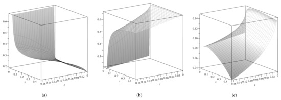
From Lemma 2, we already have that $p_1+p_2+p_3\le 1$. Therefore, it suffices to prove that $p_1,p_2,p_3\ge 0$. Because of the complex expressions of $p_1,p_2,p_3$, we prefer to show this graphically by using the Maple function plot3d. See Figure 6, where the 3D graphs of $p_1,p_2,p_3$ as functions of $(x,z)$ are plotted in the domain $\left\{\right(x,z):z/3\le x\le 1/2,0\le z\le 1/6\}$. □

Figure 6. Graphs of $p_1,p_2,p_3$ as functions of x and z. (a) $p_1$, (b) $p_2$, (c) $p_3$.

4.4. The Second Main Result

Now let us summarize the results of this section. For clarity, recall the main notations:

$$\begin{array}{cc}\hfill x_1& =x_1(x,h)=x+\frac{3(1-x){\sigma }^{2}h}{4}+\frac{2x{\sigma }^{2}h}{3}-\sqrt{3x(1-x){\sigma }^{2}h},\hfill \end{array}$$

(50)

$$\begin{array}{cc}\hfill x_2& =x_2(x,h)=x+\frac{17x{\sigma }^{2}h}{12},\hfill \end{array}$$

(51)

$$\begin{array}{cc}\hfill x_3& =x_3(x,h)=x+\frac{3(1-x){\sigma }^{2}h}{4}+\frac{2x{\sigma }^{2}h}{3}+\sqrt{3x(1-x){\sigma }^{2}h}.\hfill \end{array}$$

(52)

To distinguish the functions $x_{1,2,3}$ from $x_{1,2}$ given by (18), here we denote the latter by

$$\begin{array}{cc}\hfill y_{1,2}=y_{1,2}(x,h)& =x+(1-x){\sigma }^{2}h\mp \sqrt{(x+(1-x){\sigma }^{2}h)(1-x){\sigma }^{2}h}.\hfill \end{array}$$

(53)

Using the symmetry $S_t^x\stackrel{d}{=}1-S_t^{1-x}$ for $x\in [0,1],$ we define the approximation of the stochastic part of the WF equation as follows:

$$\begin{array}{cc}\hfill {\widehat{S}}_h^x& :=\left\{\begin{array}{cc}{x}_{1,2,3}(x,h)\mathrm{with} \mathrm{probabilities} p_{1,2,3}\left(34\right)\mathrm{and}\hfill & \\ 0\mathrm{with} \mathrm{probability}{p}_0=1-(p_1+p_2+p_3),\hfill & x\in (\frac{{\sigma }^{2}h}{3},\frac{1}{2}],\hfill \\ 1-x_{1,2,3}(1-x,h)\mathrm{with} \mathrm{prob.} p_{1,2,3}(1-x,h)\mathrm{and}\hfill \\ 1\mathrm{with} \mathrm{probabilities}{p}_0=1-(p_1+p_2+p_3),\hfill & x\in (\frac{1}{2},1-\frac{{\sigma }^{2}h}{3}),\hfill \\ y_{1,2}(x,h)\mathrm{with} \mathrm{probabilities} {\tilde{p}}_{1,2}(x,h):=\frac{x}{2y_{1,2}(x,h)},\hfill & x\in [0,\frac{{\sigma }^{2}h}{3}],\hfill \\ 1-y_{1,2}(1-x,h)\mathrm{with} \mathrm{probabilities} {\tilde{p}}_{1,2}(1-x,h),\hfill & x\in [1-\frac{{\sigma }^{2}h}{3},1].\hfill \end{array}\right.\hfill \end{array}$$

(54)

Now in view of Theorem 3 and Lemmas 2–5, we can state the main result on the second-order approximation of the WF process.

Theorem 5.

Let ${\widehat{X}}_t^x$ be the discretization scheme defined by one-step approximation

$${\widehat{X}}_h^x=D(\widehat{S}(D(x,h/2),h),h/2),$$

(55)

where $D(x,h)$ is defined by (5), and $\widehat{S}(x,h)={\widehat{S}}_h^x$ is defined by (54). Then, ${\widehat{X}}_t^x$ is a second-order weak approximation of Equation (1).

4.5. Algorithm for Second-Order Approximation

In this section, we provide an algorithm for calculating ${\widehat{X}}_{(i+1)h}$ given ${\widehat{X}}_{ih}=x$ at each simulation step i:

1.

Draw a uniform random variable U from the interval [0, 1].

2.

$x:=D(x,h/2)$ (where D is given by (5))

3.

If $x\le \frac{1}{2}$, then

3.1.

if $x>\frac{{\sigma }^{2}h}{3}$, then

   $x_0:=0,$

   calculate $x_1,x_2$, $x_3$ according to (50)–(52),

   calculate $p_1,p_2$, $p_3$ according to (34),

   if $U<p_1$ then $\widehat{S}:=x_1$ else if $U<p_1+p_2$ then $\widehat{S}:=x_2$

      else if $U<p_1+p_2+p_3$ then $\widehat{S}:=x_3$ else $\widehat{S}:=x_0$

else

   calculate $y_1,y_2$ according to (53),

   $p_{1,2}:=\frac{x}{y_{1,2}(x,h)}$,

   if $U<p_1$ then $\widehat{S}:=y_1$ else $\widehat{S}:=y_2$

else

3.2.

do step 3.1 with $x:=1-x$, $x_{0,1,2,3}:=1-x_{0,1,2,3}$,

$y_{1,2}:=1-y_{1,2}$.

4.

${\widehat{X}}_{(i+1)h}:=D\left(\widehat{S},h/2\right).$

4.6. Simulation Examples

We illustrate our approximation for the test function $f\left(x\right)=x^5$. In Figure 7 and Figure 8, we compare the moments $\mathbb{E}f\left({\widehat{X}}_t^x\right)$ and $\mathbb{E}f\left(X_t^x\right)$ as functions of t (left plots, $h=0.01$) and as functions of a discretization step h (right plots) in terms of the relative error. We observe that with a rather small number of iterations, the second-order approximation agrees with the exact values pretty well. These specific examples have been chosen to illustrate the behavior of approximations with small (${\sigma }^2=0.6$) and high (${\sigma }^2=2$) volatility. In comparison with the simulation results for the first-order approximation (Section 3.3), we see that to get a similar accuracy, we can use the second-order approximation with a significantly smaller number of iterations N and larger step size h, which in turn requires significantly less computation time.

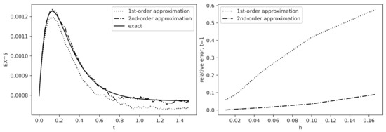
Figure 7. Comparison of $\mathbb{E}f\left({\widehat{X}}_t^x\right)$ and $\mathbb{E}f\left(X_t^x\right)$ as functions of t and h for $f\left(x\right)=x^5$: $x=0.24$, ${\sigma }^2=0.6,a=0.8,b=5$, the number of iterations $N=\mathrm{100,000}$. Left: $h=0.01$; Right: the relative error at $t=1.$

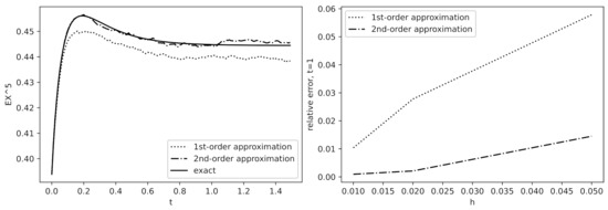
Figure 8. Comparison of $\mathbb{E}f\left({\widehat{X}}_t^x\right)$ and $\mathbb{E}f\left(X_t^x\right)$ as functions of t and h for $f\left(x\right)=x^5$: $x=0.83$, ${\sigma }^2=2,a=4,b=5$, the number of iterations $N=\mathrm{100,000}$. Left: $h=0.01$; Right: the relative error at $t=1.$

5. Probabilistic Proof of Regularity of Solutions of the Kolmogorov Backward Equation

Theorem B is in fact Theorem 1.19 of [4] stated based on the results of [7], which are proved by methods of partial differential equation theory. Here, we provide a significantly simpler probabilistic proof of the theorem for a rather wide subclass of $C^{\infty }[0,1]$, which practically includes all functions interesting for applications, for example, polynomials or exponentials.

Definition 3.

We denote by $C_{*}^{\infty }[0,1]$ the class of infinitely differentiable functions on $[0,1]$ with “not too fast” growing derivatives:

$$C_{*}^{\infty }[0,1]:=\left\{f\in C^{\infty }[0,1]:\underset{k\to \infty }{lim\; sup}\frac{1}{k!}\underset{x\in [0,1]}{max}\left|f^{\left(k\right)}\left(x\right)\right|=0\right\}.$$

Every $f\in C_{*}^{\infty }[0,1]$ is the sum of its (uniformly convergent) Taylor series:

$$f\left(x\right)=\sum _{k=0}^{\infty }{c}_k{x}^k,x\in [0,1],$$

(56)

where $c_k=f^{\left(k\right)}\left(0\right)/k!$, $k\in \overline{\mathbb{N}}$. This easily follows from the Lagrange error bound for Taylor series.

Remark 3.

Clearly, every $f\in C_{*}^{\infty }[0,1]$ is a real analytic function; see [8].

Denote $m_k(x,t):=\mathbb{E}{\left(X_t^x\right)}^k$, $k\in \overline{\mathbb{N}}$. Then, from (56), we formally have

$$\tilde{u}(t,x)=\mathbb{E}f\left(X_t^x\right)=\sum _{k=0}^{\infty }{c}_k{m}_k(x,t),x\in [0,1],t\ge 0.$$

(57)

If $\tilde{u}$ is infinitely continuously differentiable, then it satisfies Equation (2) (see, e.g., [9] (Thm. 8.1.1)). Therefore, it suffices to show that

(1)

the moments $m_k(x,t)$ are infinitely continuously differentiable and

(2)

all formal partial derivatives of the series in (57),

$$\sum _{k=0}^{\infty }{c}_k{\partial }_t^p{\partial }_x^q{m}_k(x,t),$$

(58)

converge uniformly for $(x,t)\in [0,1]\times [0,T]$ (for any fixed $T>0$).

Lemma 6.

The moments of the WF process $X_t^x$ satisfy the following recurrence relation:

$$\begin{array}{cc}\hfill m_1(x,t)& =\left\{\begin{array}{cc}x{e}^{-bt}+\frac{a}{b}(1-e^{-bt}),\hfill & 0\le a\le b\ne 0,\hfill \\ x,\hfill & a=b=0,\hfill \end{array}\right.\hfill \end{array}$$

(59)

$$\begin{array}{cc}\hfill m_k(x,t)& =e^{-b_{k}t}\left(x^k+a_k{\int }_0^t{e}^{b_{k}s}{m}_{k-1}(x,s)ds\right),k\ge 2,\hfill \end{array}$$

(60)

where $b_k=kb+k(k-1)\frac{{\sigma }^2}{2},a_k=ka+k(k-1)\frac{{\sigma }^2}{2}$.

In particular, by induction on k it follows that $m_k(x,t)$ are infinitely continuously differentiable with respect to $(x,t)\in [0,1]\times {\mathbb{R}}_{+}$.

Proof. 

Taking the expectations of both sides of Equation (1) and then differentiating with respect to t, we get

$$\begin{array}{cc}\hfill {\partial }_t{m}_1(x,t)& =a-b{m}_1(x,t),m_1(x,0)=x.\hfill \end{array}$$

Solvingthe latter, we get (59).

When $k\ge 2$, by Itô’s formula, we have

$$\begin{array}{cc}\hfill {\left(X_t^x\right)}^k& =x^k+k{\int }_0^t{\left(X_t^x\right)}^{k-1}d{X}_s^x+\frac{1}{2}k(k-1){\int }_0^t{\left(X_t^x\right)}^{k-2}d{⟨X^x⟩}_s\hfill \\ \hfill & =x^k+k{\int }_0^t{\left(X_t^x\right)}^{k-1}(a-b{X}_s^x)\mathrm{d}s+k\sigma {\int }_0^t{\left(X_t^x\right)}^{k-1}\sqrt{X_s^x(1-X_s^x)}\mathrm{d}{B}_s\hfill \\ \hfill & +\frac{1}{2}k(k-1){\sigma }^2{\int }_0^t{\left(X_t^x\right)}^{k-2}{X}_s^x(1-X_s^x)\mathrm{d}s\hfill \\ \hfill & =x^k+k{\int }_0^t\left(a{\left(X_t^x\right)}^{k-1}-b{\left(X_s^x\right)}^k\right)\mathrm{d}s+k\sigma {\int }_0^t{\left(X_t^x\right)}^{k-1}\sqrt{X_s^x(1-X_s^x)}\mathrm{d}{B}_s\hfill \\ \hfill & +\frac{1}{2}k(k-1){\sigma }^2{\int }_0^t\left({\left(X_t^x\right)}^{k-1}-{\left(X_s^x\right)}^k\right)\mathrm{d}s.\hfill \end{array}$$

By taking the expectations, we get

$$\begin{array}{cc}\hfill m_k(x,t)& =x^k+{\int }_0^t\left\{[ka+k(k-1)\frac{{\sigma }^2}{2}]m_{k-1}(x,s)-[kb+k(k-1)\frac{{\sigma }^2}{2}]m_k(x,s)\right\}\mathrm{d}s\hfill \\ \hfill & =x^k+{\int }_0^t\left\{a_k{m}_{k-1}(x,s)-b_k{m}_k(x,s)\right\}\mathrm{d}s,\hfill \end{array}$$

and thus

$$\begin{array}{c}\hfill {\partial }_t{m}_k(x,t)=-b_k{m}_k(x,t)+a_k{m}_{k-1}(x,t),m_k(x,0)=x^k.\end{array}$$

Solving the latter with respect to $m_k$, we arrive at (60). □

Lemma 7.

All formal partial derivatives of the series (57),

$$\sum _{k=0}^{\infty }{c}_k{\partial }_t^p{\partial }_x^q{m}_k(x,t),$$

(61)

converge uniformly for $(x,t)\in [0,1]\times [0,T]$ (for any fixed $T>0$).

Proof. 

It is obvious that $0\le m_k(x,t)\le 1,x\in [0,1],k\in \overline{\mathbb{N}}$. First, consider the derivatives with respect to x. Let us prove by induction on k that

$${\partial }_x{m}_k(x,t)\le k,x\in [0,1],k\in \mathbb{N}.$$

For $k=1$, we have $m_1^{\prime }(x,t)=e^{-bt}\le 1$. Suppose

$${\partial }_x{m}_{k-1}(x,t)\le k-1,x\in [0,1].$$

Then,

$$\begin{array}{cc}\hfill {\partial }_x{m}_k(x,t)& =e^{-b_{k}t}\left(k{x}^{k-1}+a_k{\int }_0^t{e}^{b_{k}s}{\partial }_x{m}_{k-1}(x,s)\mathrm{d}s\right)\hfill \\ \hfill & \le e^{-b_{k}t}\left(k+a_k(k-1){\int }_0^t{e}^{b_{k}s}\mathrm{d}s\right)=e^{-b_{k}t}\left(k+\frac{a_k}{b_k}(k-1)(e^{b_{k}t}-1)\right)\hfill \\ \hfill & \le e^{-b_{k}t}k+k(1-e^{-b_{k}t})=k,\hfill \end{array}$$

where we used the fact that $0\le a_k\le b_k$, since $0\le a\le b$.

Similarly, by induction on k, we can prove that

$$\begin{array}{c}\hfill {\partial }_x^l{m}_k(x,t)\le {\left(k\right)}_l=k(k-1)\dots (k-l+1),x\in [0,1],k\in \mathbb{N},l\in \mathbb{N}.\end{array}$$

Indeed, for $k=1$, ${\partial }_x{m}_1(x,t)=e^{-bt}\le 1={\left(1\right)}_1$, and ${\partial }_x^l{m}_k(x,t)=0={\left(1\right)}_l$ for $l\ge 2$. Now suppose that for some k,

$${\partial }_x^l{m}_{k-1}(x,t)\le {(k-1)}_l,x\in [0,1],l\in \mathbb{N}.$$

Then,

$$\begin{array}{cc}\hfill {\partial }_x^l{m}_k(x,t)& =e^{-b_{k}t}\left(k(k-1)\dots (k-l+1)x^{k-l}+a_k{\int }_0^t{e}^{b_{k}s}{\partial }_x^l{m}_{k-1}(x,s)\mathrm{d}s\right)\hfill \\ \hfill & \le e^{-b_{k}t}\left(k(k-1)\dots (k-l+1)+\frac{a_k}{b_k}k(k-1)\dots (k-l+1)(e^{b_{k}t}-1)\right)\hfill \\ \hfill & \le k(k-1)\dots (k-l+1)={\left(k\right)}_l.\hfill \end{array}$$

Now let us differentiate the moments with respect to t. We have

$$\begin{array}{cc}\hfill |{\partial }_t{m}_1(x,t)|& =\left|{\left(e^{-bt}\left(x-\frac{a}{b}\right)+\frac{a}{b}\right)}_t^{\prime }\right|=|-b{e}^{-bt}\left(x-\frac{a}{b}\right)|\hfill \\ \hfill & =|(a-bx)e^{-bt}|\le b,x\in [0,1];\hfill \\ \hfill |{\partial }_t{m}_k(x,t)|& =|-b_k{e}^{-b_{k}t}\left(x^k+a_k{\int }_0^t{e}^{b_{k}s}{m}_{k-1}(x,s)\mathrm{d}s\right)+e^{-b_{k}t}{a}_k{e}^{b_{k}t}{m}_{k-1}(x,t)|\hfill \\ \hfill & \le b_k{e}^{-b_{k}t}{x}^k+a_k{b}_k{e}^{-b_{k}t}{\int }_0^t{e}^{b_{k}s}\mathrm{d}s+a_k\hfill \\ \hfill & \le b_k+a_k{e}^{-b_{k}t}(e^{b_{k}t}-1)+a_k\le 3b_k;\hfill \\ \hfill |{\partial }_t^2{m}_k(x,t)|& =|b_k^2{e}^{-b_{k}t}\left(x^k+a_k{\int }_0^t{e}^{b_{k}s}{m}_{k-1}(x,s)\mathrm{d}s\right)\hfill \\ \hfill & -a_k{b}_k{m}_{k-1}(x,t)+a_k{\partial }_t{m}_{k-1}(x,t)|\hfill \\ \hfill & \le b_k^2+b_k{a}_k+b_k{a}_k+3a_k{b}_k\le 6b_k^2,\hfill \\ \hfill |{\partial }_t^3{m}_k(x,t)|& \le |b_k^3{e}^{-b_{k}t}\left(x^k+a_k{\int }_0^t{e}^{b_{k}s}{m}_{k-1}(x,s)ds\right)+a_k{b}_k^2{m}_{k-1}(x,t)\hfill \\ \hfill & +a_k{b}_k{\partial }_t{m}_{k-1}(x,t)+a_k{\partial }_t^2{m}_{k-1}(x,t)|\le 12b_k^3,\hfill \end{array}$$

and by induction

$$\begin{array}{cc}\hfill |{\partial }_t^l{m}_k(x,t)|& \le 3\times 2^{l-1}{b}_k^l.\hfill \end{array}$$

Finally, for all mixed partial derivatives, we have

$$\begin{array}{cc}\hfill |{\partial }_t^p{\partial }_x^q{m}_k(x,t)|& =\left|{\partial }_t^p{\partial }_x^q{e}^{-b_{k}t}\left(x^k+a_k{\int }_0^t{e}^{b_{k}s}{m}_{k-1}(x,s)ds\right)\right|\hfill \\ \hfill & \le \left|{\partial }_t^p{e}^{-b_{k}t}\right(k(k-1)\dots (k-q+1)\hfill \\ \hfill & +a_k(k-1)(k-2)\dots (k-q){\int }_0^t{e}^{b_{k}s}ds\left)\right|\hfill \\ \hfill & \le \left|{\partial }_t^p{e}^{-b_{k}t}\left(k(k-1)\dots (k-q+1)\left(a_k{\int }_0^t{e}^{b_{k}s}ds+1\right)\right)\right|\hfill \\ \hfill & =|{(-b_k)}^p{e}^{-b_{k}t}\left(k(k-1)\dots (k-q+1)\left(a_k{\int }_0^t{e}^{b_{k}s}ds+1\right)\right)\hfill \\ \hfill & +k(k-1)\dots (k-q+1)a_k|\hfill \\ \hfill & =(b_k^p+1)k(k-1)\dots (k-q+1)a_k=O\left(k^{2p+q+2}\right),k\to \infty .\hfill \end{array}$$

Since $c_k=o(1/k!)$, we have that

$$\sum _{k=1}^{\infty }{c}_k{k}^{2p+q+2}<+\infty ,$$

and by the Weierstrass M-test it follows that, indeed, the function series (61) converges uniformly for all $p,q\in \overline{\mathbb{N}}$. □

6. Conclusions

We have constructed first- and second-order weak split-step approximations of the Wright–Fisher (WF) process. The approximations use generation of a two- or three-valued random variable at each discretization step. The main difficulty was ensuring that the values of approximations take values in [0, 1], the domain of the WF process. Illustrative simulations show perfect accuracy of the constructed approximations.

References

- Milstein, G.N.; Tretyakov, M.V. Stochastic Numerics for Mathematical Physics; Springer: Berlin/Heidelberg, Germany, 2004. [Google Scholar]
- Alfonsi, A. Affine Diffusions and Related Processes: Simulation, Theory and Applications; Bocconi & Springer Series; Springer: Cham, Switzerland, 2015. [Google Scholar]
- Cox, J.C.; Ingersoll, J.E.; Ross, S.A. A theory of the term structure of interest rates. Econometrica 1985, 53, 385–407. [Google Scholar] [CrossRef]
- Alfonsi, A. High order discretization schemes for the CIR process: Application to affine term structure and Heston models. Math. Comput. 2010, 79, 209–237. [Google Scholar] [CrossRef]
- Lileika, G.; Mackevičius, V. Weak approximation of CKLS and CEV processes by discrete random variables. Lith. Math. J. 2020, 60, 208–224. [Google Scholar] [CrossRef]
- Lileika, G.; Mackevičius, V. Second-order weak approximations of CKLS and CEV processes by discrete random variables. Mathematics 2021, 9, 1337. [Google Scholar] [CrossRef]
- Epstein, C.L.; Mazzeo, R. Wright–Fisher diffusion in one dimension. SIAM J. Math. Anal. 2010, 42, 568–608. [Google Scholar] [CrossRef]
- Krantz, S.G.; Parks, H.R. A Primer of Real Analytic Functions, 2nd ed.; Birkhäuser: Boston, MA, USA, 2002. [Google Scholar]
- Ksendal, B. Stochastic Differential Equations: An Introduction with Applications, 5th ed.; Springer: Berlin/Heidelberg, Germany; New York, NY, USA, 2000. [Google Scholar]
Publisher’s Note: MDPI stays neutral with regard to jurisdictional claims in published maps and institutional affiliations. |
© 2022 by the authors. Licensee MDPI, Basel, Switzerland. This article is an open access article distributed under the terms and conditions of the Creative Commons Attribution (CC BY) license (https://creativecommons.org/licenses/by/4.0/).