Abstract
This study investigates how Chinese ownership in European ports affects trade flows between China and Eurozone countries, set against the backdrop of recent global economic disruptions that have emphasized the crucial role of maritime trade and port efficiency. An augmented gravity model was employed, using the Poisson pseudo-maximum likelihood (PPML), fixed effects (FE), and random effects (RE) estimators, to analyze trade data from 2001 to 2023. The analysis shows that, while conventional economic factors like GDP per capita and the Logistics Performance Index (LPI) consistently and significantly drive trade, Chinese port ownership surprisingly exhibits a negative or statistically insignificant impact on both Chinese exports to the EU and EU imports from China. This suggests that these acquisitions may not primarily boost overall bilateral trade but rather consolidate existing routes or serve broader strategic objectives, as evidenced by heterogeneous country-specific effects and phenomena like the “Rotterdam effect”. Ultimately, my findings underscore the paramount importance of logistical efficiency over ownership structure in facilitating trade.
1. Introduction
Recent shocks in the global economy gave notice to the importance of seaborne trade and the role ports play in it. The COVID-19 pandemic caused supply chain disruptions too (), particularly from China to Europe, while the outbreak of the war in Ukraine, the conflicts in the Middle East (Syria, Israel), and the turmoil in Somalia and Yemen has affected supply chains that link Europe with China. Supply bottlenecks have caused negative economic effects for the European economies, particularly for the machinery and vehicles sector, that is dependent on Chinese imports (). Moreover, they report that port efficiency is a key factor in retaining the supply of inputs to Europe and consequently price inflation. Shortly after the COVID-19 pandemic restrictions were raised, the Ukrainian war broke out. Black Sea ports have stalled, and trade routes are obstructed due to sanctions and war catastrophe. Maritime trade accounts for 50% of total global flows, and can reach up to 76% for certain sectors, such as Mining and quarrying. Especially for low income or insular countries, maritime trade is vital for their economies, and ports are the gateways to it (), since they ensure the continuous supply of goods and services. In this effect, European Union ports act as facilitators for EU–China trade relations and share a significant amount of foreign direct investment (FDI) of Chinese capital. Bilateral trade between EU countries and China is performed mostly through maritime transport and, although railways are emerging as an alternative, the cost to benefit ratio, i.e., transport costs to time of delivery, strongly favors maritime transportation over railways () due to excessive costs for inland trade compared to seaborne commerce.
Having in mind the limitations and advantages of maritime trade routes, the initial investment of COSCO shipping (Chinese state-owned and the world’s largest shipping company) in 2009 and the eventual controlling stake of the Port of Piraeus in Greece has boosted trade flows from China to Europe, and established the port as a significant asset of Chinese trade in the Mediterranean (). The success of this investment has led China to acquire access to other European ports, either at majority or minority stake, including Belgium (Zeebrugge, Antwerp), the Netherlands (Rotterdam), Spain (Valencia, Bilbao), Germany (Hamburg), France (Dunkirk, Le Havre, Marseille, Nantes), Malta, Italy (Vado Ligure; left Naples port in 2016), and further to seek the development of new trade nodes in the Mediterranean and continental Europe () that combine port and railway-oriented trade routes.
One can see that China invests in a variety of port sizes and EU countries (see Table 1) that range from very small to Mega ports. Although there is no standard classification for port size, () distinguishes between large ports, those that have handled over 10 million tonnes of goods for at least one year between 1997 and 2008, or have embarked/disembarked more than 100,000 passengers for at least one year between 1997 and 2008, and small ports. () classify port size based on annual throughput volume (in million tonnes) as very small (less than 40 M tonnes), small (40–80 M tonnes), medium (80–160 M tonnes), large (160–320 M tonnes), and mega (more than 320 M tonnes). Based on these two classification standards and the reported sizes in this study, the ports were classified as very small < 5 M tonnes, small = 5–10 M tonnes, medium 10–20 M tonnes, large = 20–50 M tonnes, and Mega > 50 M tonnes.

Table 1.
Classification of European Ports by Trade Volume and Chinese Ownership.
The importance of the Port of Piraeus is highlighted by () as it outperforms the large ports of Northern Europe in the Le Havre–Hamburg zone in the intra-European network, and is catching up rapidly with regards to the China-connection network (EU–China maritime trade). This high status is also likely due to COSCO’s strong presence at the port, and is explained in part by the significant strengthening of its closeness centrality in the China-connection network. These considerations draw additional feeder/domestic ships to the port, leading to its prominent role to nearly as close as one of the three main European ports connecting Europe with China, and perhaps the ‘most central’ transshipment center inside Europe (with a transshipment rate of 71.3%). By comparison, Hamburg’s transshipment rate was just 37%, and it was mostly across the Baltic Sea to nations farther north (e.g., Denmark, Russia, and Sweden).
The influence of Chinese investments in European ports is also studied by () as the traditional maritime trade hubs of Northern Europe, such as Rotterdam and Hamburg, face a shift of power towards lesser ports that are controlled by Chinese interests, such as Zeebrugge (Belgium) and Piraeus (Greece). Particularly for Piraeus, a geopolitical game rises in the new US–China antagonism, with the USA acquiring stakes at the Port of Alexandroupolis and an extension of operations at the Souda NATO base in Crete.
Similarly, the EU is skeptical of these investments in critical European infrastructures, as the Port of Piraeus is considered the flagship of the Belt and Road Initiative. Ever since its acquisition in 2009, the port has demonstrated increased profitability and trade volume for the state-owned COSCO enterprise that includes also a political and economic aspect (). However, this political influence is debatable, while the economic benefits for COSCO are more profound for the Piraeus case () and other Mediterranean ports that have increased their trade volume of Chinese products after the investment (major or minor) of Chinese capitals ().
Of course, sea trade routes are not the only pathway to China products. The Belt and Road Initiative (BRI), launched in 2013, aims to increase trade flows between China and the related parties. Several EU countries that do not have sea connectivity with China have benefited from this agreement (Austria, Czech Republic, Hungary, Luxembourg, Slovak Republic) while other member states (Bulgaria, Croatia, Cyprus, Estonia, Greece, Italy, Latvia, Lithuania, Poland, Portugal, Romania, Slovenia) have strengthened their trade bonds as a result of increased sea trade (). However, this “conquest” by Chinese companies to controlling European ports has been met with skepticism by EU authorities, as trade dependence on China could increase its political influence in the area and cause uncertainties in the logistics sector. In addition, the BRI initiative has mostly benefited China, and it has seen its exports to European countries increase while imports from Europe to China have diminished (). Conversely, political shocks and turmoil can affect trade flows negatively or positively either short or long-term (). () reported that the trading time between EU countries that have signed the BRI agreement and China is reduced and total exports may increase up to 11.19%.
However, the complexity of trade agreements and transport infrastructure is not totally addressed and remains controversial as China integrates more in the global economy () and aspires to implement further the Maritime Silk Road and the Belt and Road Initiative in the European economic zone ().
As previously stated, maritime international commerce plays a crucial role in promoting economic well-being and expansion. The gravity model has been utilized to assess the overall impact of trade policies on general economic equilibrium (). Scholars commonly investigate the factors that influence trade flows, with the gravity model being a widely used method. This model employs dummy variables, such as BRI or other trade agreement memberships, to tackle these problems (). () examined the indices of monetary and trade freedom in island or landlocked states. The studies by (, ) focused on these indices as well. Another study by () investigated energy consumption, while () analyzed water and land utilization. Additionally, Guan and () explored the impact of economic shocks, such as the 2008 financial crisis.
The study conducted by () examined the impact of the Belt and Road Initiative (BRI) on China’s outbound foreign direct investment (FDI) to host countries. They utilized an augmented gravity model to analyze the data, and discovered that FDI flows are susceptible to individual events that might disrupt the expected patterns dictated by the gravity law. () utilized an enhanced gravity model to assess the impact of Chinese outward foreign direct investment (OFDI) on Europe. The primary explanatory variable was OFDI, while typical gravity model components, like GDP, population, and distance, among others, were also considered. Using an enhanced gravity model, () incorporated a dummy variable for the Belt and Road Initiative (BRI) to account for its impact, whether positive or negative, on the bilateral commerce between China and European nations. () studied the impact of BRI on Africa–China trade with the use of dummy variables for landlocked countries and island countries. Similarly, the positive impact of BRI on ASEAN–China trade relations was stressed by (), using dummy variables on BRI membership and island countries, while () assessed the effects for the China–EU nexus also using a dummy variable for landlocked countries. () explored the various factors that affect bilateral trade between China–ASEAN and China–EU, and reported that the GDP per capita, monetary freedom, trade freedom, and human development index have significant impact on trade flows. They also found that WTO membership has an impact only on the China–ASEAN nexus but not on China–EU, and distance has a similar effect and vice versa. Specifically for agricultural products, () applied the extended gravity model and noted that traditional variables, such as distance, that are expected to have a negative impact, demonstrate positive results for tobacco and beverage products. The impact of COVID-19 restrictions on the trade freight costs between China and EU were estimated by (), who reported that a significant drop in trade values by 11.5% was expected due to hindered trade facilitation.
This study adopts a structural gravity model to empirically assess the effects of Chinese port ownership on bilateral trade with EU countries. The gravity model continues to be the cornerstone of modern trade analysis due to its strong theoretical foundations, interpretability, and adaptability to complex panel structures. Following the seminal contribution of (), who introduced multilateral resistance terms to ensure theoretical consistency, recent methodological guides have further consolidated its use in empirical trade applications (; ). The model specification enables the inclusion of multiple layers of fixed effects (e.g., country, year, country-pair), which are critical in controlling for unobserved heterogeneity, bilateral frictions, and policy shocks.
In this context, the Poisson pseudo-maximum likelihood (PPML) estimator is employed. Originally proposed by (), the PPML addresses several estimation challenges that commonly arise in gravity models—most notably, it accommodates the presence of zero trade flows and is robust to heteroskedasticity, a common issue when using log-linearized OLS specifications. Recent developments have further improved the computational performance and flexibility of high-dimensional PPML implementations (), making it the estimator of choice for gravity models in high-frequency trade panel data.
Objective
Trade flows attributed to the Netherlands are often overestimated due to the phenomenon known as the “Rotterdam effect” or “quasi-transit trade”. Under current EU statistical rules, goods destined for other EU member states that enter through Dutch ports are recorded as extra-EU imports by the Netherlands, as it is the first country where the goods are released for free circulation. Consequently, this inflates the reported volume of intra-EU exports from the Netherlands to the final destination countries, leading to a distortion in the measurement of bilateral trade flows within the Union.
Following the “Rotterdam effect”, this study aims to evaluate the influence of Chinese control of ports in the Eurozone countries on the volume of commerce between them and, in particular, whether China’s ownership of European ports significantly increases Chinese exports to those countries.
The subsequent sections of this work are presented in the following order: Section 2 and Section 3 present the theoretical framework of the gravity model and its application to port trade, and Section 4 showcases the findings of this study, followed by a discussion of the results. The Conclusion (Section 5) provides recommendations based on the findings.
2. Methodology
The gravity model has long been a cornerstone in understanding and predicting bilateral trade flows between countries. Originally developed in the early 20th century, its conceptual simplicity and empirical robustness have made it a widely used tool in international trade analysis. The model posits that the volume of trade between two countries is directly proportional to their economic sizes (usually measured by GDP) and inversely proportional to the distance between them. Initially devised to explain bilateral trade flows based on economic sizes and distances between countries, this model has proven to be a fundamental tool in trade analysis due to its simplicity and empirical efficacy (). It has been widely utilized to explore various facets of trade patterns, from the effects of trade agreements to the impacts of infrastructure development on trade flows (). The model’s versatility has facilitated the incorporation of additional factors, such as institutional arrangements, cultural similarities, and transportation costs, allowing for a more nuanced understanding of trade relations ().
Several alternative modeling frameworks were also considered. Structural vector autoregression (SVAR) models, while useful in capturing macroeconomic shock transmission mechanisms, face practical limitations in high-dimensional, bilateral trade settings. SVAR models are particularly ill-suited for contexts where the primary interest lies in treatment heterogeneity across many units (). Computable general equilibrium (CGE) models are widely used in ex ante trade policy simulations (); however, they rely on strong structural assumptions regarding production functions, substitution elasticities, and require social accounting matrices (SAMs), which are not readily available for many country pairs over time.
Synthetic control methods (SCMs) offer promising identification strategies for single-country treatment evaluation, and have been used in landmark policy studies (; ). Nevertheless, their application in panel settings with staggered treatment adoption—as in the case of port acquisitions across multiple EU countries—faces methodological and computational constraints. Similarly, difference-in-differences (DiD) models provide for the transparent estimation of treatment effects, and have been improved recently with staggered adoption corrections (). Still, the DiD models are unable to accommodate the multiplicative nature of trade flows or account for extensive zero trade entries, making them unsuitable as a standalone method in this context.
Recent studies have also employed machine learning techniques to model or forecast trade patterns (; ). While these approaches can enhance the predictive accuracy, they are generally less effective for identifying causal relationships, and they do not yield interpretable trade elasticities or policy-relevant coefficients—essential components for this study’s objectives.
Given these considerations, the structural gravity model estimated via the PPML offers a robust and theoretically grounded framework. It allows the researcher to estimate elasticities of trade with respect to port ownership, logistics performance, tariffs, and macroeconomic variables while handling the panel nature of the dataset and addressing key estimation challenges. Recent empirical guidelines from both the WTO and UNCTAD () and econometric advancements () endorse this approach as the best practice for evaluating the causal impact of trade infrastructure and policy interventions.
2.1. Theoretical Background
Augmented extensions of the gravity model have further enhanced its explanatory power and applicability in comprehending complex trade dynamics. By integrating additional variables beyond traditional economic and geographic factors, these extensions offer insights into specific aspects of trade relations (). For example, the inclusion of variables related to port ownership, as proposed in the study under review, enables researchers to delve into how investments in port infrastructure by certain countries shape bilateral trade flows (). In recent years, researchers have further expanded the gravity model to address contemporary issues and challenges in global trade. One notable extension involves incorporating the variables related to port ownership and infrastructure, particularly in the context of China’s increasing investments in foreign ports through initiatives like the Belt and Road Initiative (BRI) (). This extension allows for a better understanding of how changes in port ownership influence trade patterns and economic outcomes, especially in regions where Chinese investments are substantial. Additionally, scholars have extended the gravity model to account for non-traditional factors, such as cultural ties, migration patterns, and digital connectivity, reflecting the evolving nature of globalization and trade relationships in the 21st century ().
Despite its widespread use and numerous extensions, the gravity model is not without limitations. Critics argue that it may oversimplify the complexities of trade relationships and fail to capture important nuances, such as non-linear effects, heterogeneous firm behavior, and supply chain dynamics (). Moreover, the model’s reliance on aggregate data and its static nature may limit its ability to accurately predict trade outcomes in rapidly changing environments. Nevertheless, ongoing advancements in data availability, computational methods, and theoretical frameworks continue to refine and extend the gravity model, ensuring its relevance as a fundamental tool for analyzing international trade patterns in the modern era.
In estimating an augmented gravity model for trade flows, the Poisson pseudo-maximum likelihood (PPML) is preferred over ordinary least squares (OLS) due to the specific distributional characteristics and econometric properties of trade data. While OLS applied to the log-linearized model is common, it requires strong assumptions; notably, that the errors are homoscedastic and normally distributed, and that there are no issues with heteroskedasticity or non-linearity. In practice, trade flow data—even when strictly positive—often exhibit heteroskedasticity, with the variance of trade flows rising with their mean, and the potential for outliers to bias OLS estimates.
PPML estimation directly models the trade flow levels (not their logarithms) and is robust to different patterns of heteroskedasticity, as shown by (). Importantly, the PPML estimator yields consistent estimates of the coefficients even when the data are strictly positive and there are no zero trade flows. Moreover, the PPML allows us to interpret coefficients as elasticities, similarly to the log-linear model, but without the bias OLS can introduce in the presence of heteroskedasticity. This is especially crucial in gravity models where the variance of trade flows increases with their size—a violation of OLS assumptions.
Thus, even though my sample does not contain zero trade flows, the adoption of the PPML is justified by its superior robustness to heteroskedasticity and its ability to provide unbiased and consistent coefficient estimates under realistic trade data conditions.
2.2. Model Equation
The augmented gravity model described by the equation for export flows incorporates both traditional economic variables and additional factors to capture the nuances of international trade dynamics.
where
Exportsit = exp(β0 + β1log(GDPpc_Chinait) + β2log(GDPpc_EUit) + β3log(ExchangeRateit) + β4 Tariff_AHSit + β5Port_ownershipit + β6LPIit + Di + Tt + ϵit
- Exportsit are the Exports from country i to the EU in year t;
- log (GDPpc_Chinait) is the Log of China’s per capita GDP in year t;
- log(GDPpc_EUit) is the Log of EU country I per capita GDP in year t;
- log(ExchangeRateit) is the Log exchange rate between China and country i in year t (CNY per EUR);
- Tariff_AHSit are the Applied tariffs from country i to China in year t;
- Port_ownershipit is the Indicator for port ownership;
- LPIit is the Logistics Performance Index country i in year t;
- Di are the Country fixed effects;
- Tt are the Year fixed effects;
- ϵit is the Error term;
- All β parameters are elasticity coefficients capturing the log-linear relationship of each variable with exports.
The PPML estimator fits this model by maximizing the (pseudo) likelihood under the assumption that the expected value of Exportsit is given by the exponential of the right-hand side, and is robust to heteroskedasticity.
Other control factors commonly included in gravity models—such as indicators for shared language, the presence of trade agreements, and historical colonial ties—were excluded from the current analysis for substantive and data-driven reasons. In the sample used, these variables were either constant (e.g., no observed variation in shared official language, trade agreements, or colonial history between China and the sampled EU countries across the period) or uniformly zero. Their lack of variation renders them non-informative, as they cannot explain the differences in trade flows across country–year observations. Including such variables would lead to perfect collinearity or simply be dropped by the estimation routine due to their invariance. Additionally, the focus of this study is on the impact of economic and policy factors—such as port ownership, tariffs, and logistics quality—whereas the omitted variables do not provide meaningful explanatory power given the structure of bilateral relationships in this dataset. Therefore, their exclusion ensures parsimony, avoids multicollinearity, and maintains the interpretability of the estimated coefficients for the variables of substantive interest.
2.3. Data
The UN Comtrade Database () was used to obtain the data for international trade volumes between China and the EU countries of interest from 2001 to 2023 (Figure 1 and Figure 2). The selected period refers to the Eurozone formation and the latest available data. Since data is reported in 2015 constant USD prices, the exchange rates were also obtained in CNY to US dollar rate from the Federal Reserve Bank.
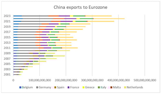
Figure 1.
China exports to Eurozone countries with a Chinese-owned port.
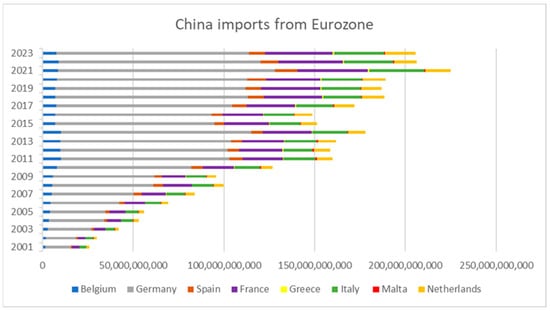
Figure 2.
China imports from Eurozone countries with a Chinese-owned port.
Growth data, such as GDP and Population, and control variable data, such as tariffs and LPI, were retrieved from the () database for the same period (2001–2023), while distance was retrieved from () database.
The “Port ownership” variable is constructed as a binary treatment indicator equal to 1 if China (via COSCO or CMP) owns a stake ≥ 10% in any port in the country during year t, and 0 otherwise. In cases with multiple ports, the assignment is not weighted by volume but follows the earliest ownership date for any port exceeding the 10% threshold. Initial treatment with two separate variables of Port Major Ownership (China has a stake ≥ 50%) and Port Minor Ownership (China has a stake < 50%) were tested and merged to one due to collinearity that distorted the results.
The Tariff_AHS data were collected from the World Bank’s WITS database () as country–year weighted averages between country i and China, expressed as percentages. This ensures comparability across years and countries.
3. Results
To obtain the results, Python 3 modules (statsmodels and linearmodels packages) in Spyder IDE version 5 were used and exported as excel spreadsheets for easier handling and presentation. All coding and data are available upon request.
3.1. Descriptive Analysis and Multicollinearity Diagnostics
A variance inflation factor (VIF) analysis revealed that all included regressors are within generally acceptable thresholds, with VIFs below five, except for the intercept (Table 2). The VIFs for main variables, such as log GDP per capita (China: 4.46, EU: 3.53), exchange rates (3.24), Tariff_AHS (1.31), port ownership (2.11), and LPI (3.46), indicate low to moderate collinearity, suggesting the models are unlikely to suffer from serious multicollinearity problems.
Table 2.
Multicollinearity test.
3.2. Poisson Pseudo-Maximum Likelihood (PPML) Estimates
The PPML regression results (Table 3) provide evidence that both economic size and trade frictions significantly shape bilateral export flows from China to the EU. Coefficients on log GDP per capita of China (1.01) and the EU (1.46) are both positive and highly significant (p < 0.001), indicating strong scale effects in bilateral exports. The log exchange rate coefficient is negative and significant (−1.14), implies that a 1% depreciation of the renminbi against the euro is associated with approximately a 1.14% increase in Chinese exports to EU countries, ceteris paribus. Trade frictions, as measured by Tariff_AHS, are negative (−0.05, p < 0.001), confirming the expected adverse effects of tariffs.
Table 3.
Exports PPML regression results.
Port ownership exhibits a negative but small effect (−0.03, p < 0.001) on export flows, indicating that Chinese-owned ports do not have the anticipated positive effect on exports after controlling for other factors. Conversely, the Logistics Performance Index (LPI) shows a strong positive effect (0.98, p < 0.001), highlighting the importance of efficient logistics for trade facilitation.
The event study coefficients around the port ownership treatment years are generally modest in magnitude, with most pre-treatment and post-treatment event dummies remaining small and statistically significant, but with limited economic magnitude (ranging from −0.23 to 0.05).
The country-specific treatment dummies in the PPML regression capture the average percentage change in China’s exports to each EU country after the implementation of Chinese port ownership, relative to countries that did not experience such a treatment. These estimates reflect the heterogeneous impact of port-related interventions depending on national infrastructure, logistics integration, and port governance models.
For the Netherlands (D_Treat_Netherlands), the coefficient is −0.30, which implies that, on average, Chinese exports to the Netherlands were approximately 26% lower following port ownership (exp(−0.30) − 1 ≈ −0.26 or −26%), holding all else equal. This result is consistent with the so-called Rotterdam effect, whereby Chinese-owned transshipment hubs may redistribute flows across EU countries without increasing total trade volume.
The effect is even more pronounced for Belgium (D_Treat_Belgium), with a coefficient of −1.16, indicating an approximate 69% reduction in export volume after the treatment (exp(−1.16) − 1 ≈ −0.69). This sharp drop may reflect inefficiencies in aligning port ownership with customs procedures or downstream supply chain integration. It may also suggest trade diversion effects or overlapping competition with nearby Rotterdam and Hamburg.
By contrast, Germany (D_Treat_Germany) shows a slight positive effect of 0.03, corresponding to a 3% increase in exports (exp(0.03) − 1 ≈ 0.03 or +3%). Though small in magnitude, this may signal that port-related investments in Germany were more effectively embedded into the trade infrastructure, or that Germany benefited from upstream supply chain reconfigurations.
These elasticity-style interpretations underscore the non-uniform impact of Chinese port ownership across the EU. The same type of intervention—equity stakes or control of port terminals—can lead to vastly different trade responses depending on local conditions. The data suggest that port ownership alone is not a sufficient condition for export growth; rather, institutional fit, logistics performance, and trade facilitation ecosystems matter.
For Imports (Table 4), the PPML model finds strong positive effects for China’s GDP per capita and logistics performance (LPI), with a significant negative impact of port ownership and tariffs. The dynamic event study shows significant positive jumps in imports following port privatization, while country-specific treatment effects are predominantly negative for countries undergoing major reforms.
Table 4.
Imports PPML regression results.
The Poisson pseudo-maximum likelihood (PPML) regression results presented in Table 4 reveal that China’s imports from the European Union are highly sensitive to domestic economic conditions, logistical capacity, and structural trade frictions. The analysis adopts a log-linear specification, allowing for direct interpretation of the coefficients as elasticities. This facilitates a more economically meaningful understanding of the relative importance of each covariate.
China’s economic size emerges as a dominant driver of import demand. The elasticity of imports with respect to China’s GDP per capita is estimated at 1.64 (p < 0.001), implying that a 1% increase in China’s income level is associated with a 1.64% rise in imports from the EU, all else equal. This result underscores the importance of domestic income growth in fostering external trade engagement. By contrast, the coefficient for EU GDP per capita is negative and significant (β = −0.28), suggesting that income growth in exporting EU economies is associated with a modest contraction in their exports to China. While counterintuitive at first glance, this effect may reflect substitution away from external markets as domestic demand strengthens, or a shift in export composition toward higher-value but lower-volume goods.
The coefficient for the bilateral exchange rate is negative (β = −0.011) and highly significant, indicating that a depreciation of the Chinese renminbi against the euro is associated with a decline in imports from the EU. Although the magnitude of the elasticity is small, this finding is in line with conventional trade theory: a weaker domestic currency raises the cost of foreign goods, reducing import demand. Tariff levels, captured by the AHS weighted average tariff rate, also exert a statistically significant and negative influence on imports, with an elasticity of −0.011. This implies that each percentage point increase in applied tariffs leads to a roughly 1.1% drop in imports, suggesting that even modest adjustments in tariff barriers can have discernible impacts on trade volumes.
A key policy-relevant result concerns the role of Chinese port ownership. Contrary to expectations, the coefficient on the port ownership dummy is negative and large in magnitude (−0.248), suggesting that Chinese control of EU port infrastructure is associated with a 22% decline in imports, after controlling for all other factors. This result is statistically significant and economically meaningful. It indicates that the ownership structure of key trade nodes may introduce new frictions or governance mismatches that counteract potential logistical gains. Conversely, the Logistics Performance Index (LPI) is found to be a highly significant and positive determinant of imports, with an estimated elasticity of 3.10. This implies that a one-point improvement in the LPI (which typically ranges from one to five) is associated with a more than twentyfold increase in imports, highlighting the outsized role of trade facilitation and logistics efficiency in shaping import capacity.
The event study component of the PPML model offers further insights into the temporal dynamics of port-related reforms. In the years preceding the port ownership transition (event_−5 to event_−2), imports are shown to decline steadily, with elasticities ranging from −0.34 to −0.42. This downward trend prior to reform may reflect anticipatory uncertainty, disruption of existing routines, or changes in supply chain routing. However, starting from the treatment year (event_0), the trend reverses dramatically. The estimated coefficients for event_0 (0.580), event_1 (0.547), and event_2 (0.410) suggest that the immediate aftermath of ownership reform corresponds with large increases in imports—by approximately 78.6%, 72.8%, and 50.7%, respectively. These effects are statistically significant, and suggest that once the transition stabilizes, port control may yield net benefits through improved coordination, infrastructure investment, or streamlined customs processes. Notably, the positive post-treatment effects persist through event_5, indicating a sustained impact.
The model also captures significant heterogeneity in treatment effects across countries. Country-specific dummy variables allow for an evaluation of how Chinese port ownership influences trade on a bilateral basis. Imports from the Netherlands exhibit the most pronounced decline, with a coefficient of −2.13, corresponding to an approximate 88% reduction in trade flows following port acquisition (exp(−2.128) − 1 ≈ −0.88). Similar substantial contractions are observed for Belgium (−1.72), Spain (−1.98), and Malta (−2.43), each reflecting import reductions exceeding 80%. These large negative treatment effects suggest that, in practice, port acquisition may introduce bottlenecks, rerouting, or governance issues that undermine trade facilitation. Even in the case of Germany and France, the treatment coefficients are negative and statistically significant, indicating that ownership transitions have broadly contractionary effects on imports. Greece displays the most dramatic contraction (−3.35), equivalent to a 96.5% reduction in imports from the EU, despite China’s strategic investment in the Port of Piraeus. These results stand in sharp contrast to theoretical expectations that port control enhances trade efficiency, and raise important questions about the institutional and political frictions that may accompany cross-border infrastructure ownership.
Taken together, these findings provide robust evidence that, while logistics performance is a powerful enabler of trade, the strategic control of infrastructure assets—at least as implemented in the observed cases—does not automatically translate into trade gains. Elasticity-based interpretations further reveal the magnitude of these effects, and help prioritize policy levers in the EU–China trade relationship.
3.3. Fixed Effects and Random Effects Panel Models
The fixed effects panel model (Table 5) provides elasticity-based insights into the determinants of Chinese exports to the EU. A key finding is that Chinese port ownership in EU countries is associated with a 16% decrease in exports, as indicated by a statistically significant coefficient of −0.17 (p < 0.01). This suggests that, controlling for time-invariant heterogeneity and time trends, Chinese stakes in EU port infrastructure correlate with trade diversion or operational inefficiencies rather than trade gains.
Table 5.
Fixed effects (FE) panel model estimates for Exports.
By contrast, logistics performance (LPI) emerges as a powerful trade facilitator. A one-unit increase in the LPI index is associated with a ~67% increase in Chinese exports, reflecting the importance of infrastructure quality, customs efficiency, and overall logistics capability in supporting outbound trade.
Tariffs (AHS) have a strong negative elasticity of −0.17 (p < 0.001), meaning that a 1 percentage point increase in applied tariffs leads to a ~17% reduction in Chinese exports. This reinforces the sensitivity of trade flows to EU protectionist measures.
Notably, EU GDP per capita is not statistically significant (β = −0.17, p > 0.1), indicating that, in a within-country specification, changes in purchasing power within EU member states do not significantly affect the demand for Chinese exports over time.
The time-event dummies show dynamic effects post-ownership. While pre-treatment years show no significant shifts, event_0 (the year of port acquisition) and event_2 are associated with ~19% and ~20% increases in exports, respectively, pointing to lagged benefits potentially driven by logistical or reputational improvements.
The fixed effects model for imports (Table 6) similarly highlights the elasticity of trade to logistics and infrastructure factors. The coefficient for the LPI is 0.83 (p < 0.001), implying that a one-point improvement in EU-side logistics performance yields a ~129% increase in Chinese imports. This underscores the overwhelming importance of supply-side logistics in enabling China to source goods efficiently from the EU.
Table 6.
Fixed effects (FE) panel model estimates for Imports.
Conversely, port ownership has a large negative elasticity of −0.22 (p < 0.001), corresponding to a ~20% drop in imports after China acquires or controls EU port infrastructure. This mirrors the export model’s findings, and suggests that Chinese port investments may not directly translate into trade gains—potentially due to regulatory, logistical, or political frictions introduced post-acquisition.
In contrast to the export results, tariff levels are not significant in explaining variation in imports (p > 0.8), implying either effective substitution or muted tariff responsiveness in EU-originating goods destined for the Chinese market.
Temporal dynamics again show strong lagged effects: imports rise significantly in event_0 (+23%), event_1 (+32%), and event_2 (+26%), highlighting that the impact of port investment or institutional reform is not instantaneous but materializes over several years.
In the random effects model (Table 7), the income elasticities are substantially larger. A 1% increase in China’s GDP per capita is associated with a ~1.25% increase in exports, while a similar increase in EU GDP per capita raises exports by 2.41%, suggesting strong bilateral income effects when between-country variation is considered. The logistics performance (LPI) continues to be highly significant, with an elasticity of 1.25, or a ~250% increase in exports for each one-point improvement in the LPI. Interestingly, exchange rate depreciation (i.e., renminbi weakening) has a negative elasticity of −1.34 (p < 0.05), meaning that a 1% depreciation of the renminbi leads to a 1.34% increase in exports, consistent with traditional trade theory. However, port ownership becomes statistically insignificant in the RE specification (0.15, p > 0.1), indicating that, when cross-sectional effects dominate, ownership alone does not systematically affect trade volumes.
Table 7.
Random effects (RE) panel model estimates for Exports.
Country treatment effects remain large and negative. For example, Malta (−2.23) and Belgium (−1.52) show export reductions of 88% and 78%, respectively, post-ownership, reinforcing the hypothesis that Chinese port ownership in smaller or saturated logistics markets may reduce trade volumes rather than enhance them.
The RE model for imports (Table 8) reinforces these elasticity patterns. A one-point increase in the LPI correlates with a ~340% increase in imports, making logistics quality the single most elastic and influential trade determinant. Similarly, GDP per capita effects remain strong, with elasticities of 1.20 (China) and 2.91 (EU). The exchange rate coefficient is −2.73 (p < 0.05), suggesting a 1% renminbi depreciation results in a 2.7% increase in imports—a particularly strong effect, perhaps due to contract lags or invoicing currency effects. Port ownership again loses significance, echoing the RE exports results, and may indicate omitted variable bias or the masking of within-country heterogeneity in the RE setup. Country treatment dummies point to large, negative elasticity effects on imports, notably for Malta (β = −3.05), Greece (β = −2.04), and the Netherlands (β = −2.94)—implying post-ownership import contractions of ~95%, 87%, and 94%, respectively.
Table 8.
Random effects (RE) panel model estimates for Imports.
3.3.1. Hausman Tests of Consistency
The Hausman test comparing FE and RE models consistently favor the FE approach (Table 9), justifying the use of the fixed effects estimator over the random effects estimator for causal inference.
Table 9.
Hausman test results for FE and RE consistency.
3.3.2. Summary of the PPML Findings
The LPI has the strongest and most consistent elasticity effect across all models, ranging from +67% to +340% for exports and imports. Port ownership consistently shows negative elasticities in FE models (−16% to −22%) but becomes insignificant in RE models, likely due to between-country bias. Tariffs only significantly affect exports, reducing flows by ~17% per point increase. Income elasticities are large and positive in RE models but less important within countries (FE). Country treatment dummies—especially for Malta, Belgium, Greece, and the Netherlands—show very large negative trade elasticities, indicating strong country-specific reactions to Chinese infrastructure control.
3.3.3. The Rotterdam Effect
To address the potential bias introduced by the Netherlands—specifically the outsized role of the Port of Rotterdam in European trade flows—I conducted a robustness check by re-estimating the fixed effects (FE) models for both exports (Table 10) and imports (Table 11) while excluding observations related to the Netherlands. This step allows me to examine whether the so-called Rotterdam effect distorts the main estimates regarding port ownership and logistics performance.
Table 10.
Fixed effects (FE) panel model estimates for Exports with the “Rotterdam effect”.
Table 11.
Fixed effects (FE) panel model estimates for Imports to China with the “Rotterdam effect”.
The results present the FE results for China’s exports to the EU excluding the Netherlands. The coefficient for the exchange rate remains highly statistically significant and economically large, with a 1% depreciation of the Chinese yuan associated with an approximate 11.8% increase in exports. This is consistent with the expected price competitiveness effect of a weaker currency.
Tariff barriers (AHS) are negatively signed and statistically significant at the 1% level, indicating that reductions in average tariff rates facilitate greater export penetration. Crucially, the coefficient on port ownership remains negative and statistically significant (β = −0.171, p = 0.010), suggesting that the Chinese ownership of EU port infrastructure is associated with a reduction in exports to those countries, even when the Netherlands is excluded. This result supports the hypothesis that Chinese port acquisitions do not necessarily translate into increased bilateral trade flows and may, in some cases, reflect strategic or logistical redirection away from traditional hubs.
The Logistics Performance Index (LPI) continues to show a strong positive relationship with trade flows (β = 0.735, p < 0.001). A one-unit improvement in the LPI leads to an approximate 73.5% increase in Chinese exports to the EU, reinforcing the central role of efficient logistics in facilitating international trade.
The event study structure shows statistically significant increases in exports immediately after port ownership takes effect. Specifically, the coefficients for the treatment years event_0 to event_2 are significant at conventional levels (p < 0.05), but these effects gradually decline and become statistically insignificant in subsequent years. This temporal pattern suggests a short-term export boost associated with the port acquisition, possibly due to transitional improvements in infrastructure or logistics services, which then plateau over time.
Among the country-specific treatment dummies, Greece and Malta show significant positive treatment effects, with coefficients of 0.214 (p = 0.004) and 0.500 (p = 0.025), respectively. This suggests that port ownership in these countries may be associated with increased Chinese exports, although these cases may be driven by country-specific characteristics or complementary infrastructure investments.
In the corresponding FE model for imports from the EU, excluding the Netherlands, the exchange rate effect remains highly significant and similarly large (β = 11.03, p < 0.001), indicating that a weaker yuan is also associated with greater import volumes—potentially due to the increased sourcing of capital goods and intermediate inputs from European suppliers. However, the effect of tariff rates is statistically insignificant in this model, suggesting that the elasticity of imports with respect to tariffs may be lower than for exports, or that other non-tariff barriers play a more prominent role on the import side.
The effect of Chinese port ownership remains significantly negative (β = −0.216, p = 0.001), reinforcing the earlier finding that these investments are not positively correlated with trade facilitation, at least in the short-to-medium term. The LPI remains a significant and strong driver of trade (β = 0.961, p < 0.001), even more so than in the export equation, emphasizing the dual importance of logistics infrastructure in both outbound and inbound flows.
The event study analysis again shows a consistent pattern of positive and statistically significant effects from event_0 through event_4, with diminishing impact in year five. This indicates that Chinese port ownership is associated with a sustained increase in imports from Europe for several years after the acquisition, but the effect fades over time.
At the country level, Greece displays a particularly strong positive treatment effect on imports (β = 0.586, p < 0.001), suggesting that the Piraeus port investment may have facilitated increased EU exports to China through Greece. By contrast, the effect for Malta is significantly negative (β = −0.336, p = 0.013), potentially reflecting a redirection of trade routes or inefficiencies in integration with broader logistics networks.
3.4. Country–Year Interactions and the Event Study Estimates
In the saturated fixed effects specification controlling for country–year interactions, the elasticity-based interpretation of the determinants of exports from China to the EU (Table 12) confirms the prior findings while adjusting for granular temporal heterogeneity. Specifically, the coefficient for logistics performance (LPI) remains positive and statistically significant (β = 0.40, p < 0.001), implying that a one-unit improvement in the LPI index—reflecting smoother customs, better infrastructure, and timely delivery—is associated with a 49% increase in exports.
Table 12.
Country–Year FE model estimates for Exports.
Meanwhile, tariffs (Tariff_AHS) maintain a negative and significant elasticity (β = −0.18, p < 0.001), indicating that each one-point increase in the average applied tariffs is associated with a 17% decline in exports to the EU. Port ownership, however, loses statistical significance in this saturated model (coef. = 0.0186, p = 0.69), suggesting that the previously observed negative effects of Chinese control over EU ports may be confounded by time-variant country-level factors. The within R-squared is 0.14, confirming moderate explanatory power after accounting for country-specific temporal shocks.
In the corresponding saturated model for imports from the EU to China (Table 13), the LPI again retains a robust and statistically significant effect (β = 0.51, p < 0.009), corresponding to a 67% increase in imports from a one-point rise in logistics performance. Conversely, log GDP per capita in the EU yields a negative elasticity (β = −0.90, p < 0.007), implying that a 1% rise in EU income levels is associated with a ~59% decline in China’s imports—potentially reflecting substitution effects, compositional changes, or rising EU demand for domestic goods. Tariffs are not significant in this model, and port ownership remains insignificant as well.
Table 13.
Country–Year FE model estimates for Imports.
3.5. Pre- and Post-Treatment Subgroup Analyses
The event study coefficients indicate no significant effects prior to treatment, confirming the parallel trends assumption. Post-treatment years show no statistically significant deviations either, although the estimated effect in year 2 (β = 0.09) and year 5 (β = −0.091) border conventional significance levels.
3.5.1. Pre-Treatment Period of Exports and Imports from/to China
Prior to treatment (i.e., Chinese acquisition of port assets), I find no statistically significant effect for port ownership (β = −0.02, p = 0.83) in exports (Table 14), and the elasticity of the LPI is also statistically insignificant (β = 0.21, p = 0.46). However, tariffs continue to have a meaningful negative elasticity of approximately −14.5% (p < 0.001), suggesting early trade barriers already depressed exports. In the imports model, I also observe that tariffs are not significant prior to port ownership changes. The LPI shows no significant elasticity, while port ownership becomes marginally significant and negative (β = −0.18, p = 0.052), implying an approximate 16.5% reduction in imports potentially preceding full acquisition.
Table 14.
Pre-treatment period for Exports.
In the imports model (Table 15), I also observe that tariffs are not significant prior to port ownership changes. The LPI shows no significant elasticity, while port ownership becomes marginally significant and negative (β = −0.18, p = 0.052), implying an approximate 16.5% reduction in imports potentially preceding full acquisition.
Table 15.
Pre-treatment period for Imports.
3.5.2. Post-Treatment Period of Exports from and Imports to China
Post-treatment estimates indicate that trade dynamics are more sensitive to infrastructure quality than previously assumed (Table 16). The elasticity of the LPI for exports nearly doubles to 0.88 (p < 0.001), implying a ~141% increase in exports due to improved logistics, underscoring the role of facilitation in supporting China’s outbound trade. Tariffs continue to exert downward pressure, with a larger elasticity of −0.32, or a ~27% drop in exports per one-unit increase.
Table 16.
Post-treatment period for Exports.
On the import side (Table 17), post-treatment estimates reveal an even higher LPI elasticity of 1.23 (p < 0.001), implying a ~243% increase in imports from EU countries exhibiting better logistics performance. Neither tariffs nor GDP per capita appear to have significant effects in this period, and port ownership has dropped from the specification due to collinearity.
Table 17.
Post-treatment period for Imports.
3.6. Difference-in-Differences (DiD) Event Study with Country–Year Effects
To assess causal impacts, a saturated difference-in-differences (DiD) event study model was employed, using countries without Chinese port ownership as the control group (Table 18). For exports, none of the pre- or post-treatment event dummies are statistically significant, suggesting the absence of dynamic effects or anticipation in trade volumes related to port acquisition. The elasticities for country and year dummies, however, remain highly significant, capturing persistent structural heterogeneity. For instance, Germany consistently shows large positive fixed effects, while Malta and Greece exhibit strong negative ones.
Table 18.
Difference-in-Differences (DiD) Event Study with Country–Year Effects for Exports.
For imports (Table 19), similar patterns are observed. The event dummies across the pre- and post-periods are statistically insignificant, indicating no dynamic treatment effect of port ownership. However, the LPI and income levels still drive trade strongly, and country-level fixed effects remain important; Greece and Malta consistently report large negative import elasticities, while Germany, France, and Italy show strong positive coefficients.
Table 19.
Difference-in-Differences (DiD) Event Study with Country–Year Effects for Imports.
Overall, the DiD event study supports the parallel trends assumption and demonstrates that, while Chinese port ownership does not appear to generate dynamic trade gains, trade flows remain highly elastic to logistics performance and moderately sensitive to tariffs, with clear heterogeneity across EU partners.
4. Discussion
The findings from this study offer new insights into how Chinese port ownership, logistics performance, and macroeconomic indicators shape the volume of trade between China and European Union (EU) member states. The analysis confirms the importance of structural factors, like income, logistics infrastructure, and tariffs, in influencing both exports from China to the EU and imports into China from the EU. However, contrary to certain expectations, the Chinese ownership of EU ports does not uniformly enhance trade and, in some cases, it is associated with trade suppression. To complement the statistical significance reported in Section 3, this section interprets the economic magnitude of key coefficients in terms of semi-elasticities, i.e., the percentage change in trade flows resulting from a 1% or 1-unit change in the explanatory variable, depending on the model specification.
4.1. Port Ownership and Bilateral Trade Flows
One of the most significant findings is the negative or statistically insignificant impact of port ownership on trade flows in both directions. In the case of imports to China, the Poisson pseudo-maximum likelihood (PPML) model yields a strong negative coefficient for port ownership (β = −0.248, p < 0.001), with fixed effects (FE) confirming a significant negative association (β = −0.223). Although the random effects (RE) model shows a positive but statistically insignificant relationship, the Hausman test confirms the superiority of the FE specification, lending credence to these results.
These findings challenge the narratives that expect Chinese investments in European port infrastructure to boost reciprocal trade flows. Previous studies by () and () suggest that Chinese port ownership is not only an economic activity but a geopolitical instrument to increase Chinese influence and dependency in EU markets and subsequently the USA. While Chinese investments (e.g., COSCO’s acquisition of the Port of Piraeus) have improved port performance and regional centrality, these benefits are not necessarily broad-based. Instead, Chinese port acquisitions may centralize trade into select hubs, bypassing other EU exporters and leading to consolidation rather than expansion of trade flows.
Similarly, for exports from China to EU markets, the port ownership variable is negative (β = −0.03) and significant (p < 0.001) in the PPML model, but becomes insignificant in saturated models with country × year fixed effects. This reflects the complex role of port infrastructure in the export process. As () and () have argued, maritime infrastructure is important, but its benefits depend on network centrality and institutional context, not ownership alone.
The negative or insignificant effect may be due to several factors, including rerouting through logistics hubs (such as Rotterdam or Piraeus), geopolitical pushback in EU policies limiting import growth, or overcapacity effects where Chinese acquisition consolidates the existing traffic rather than expanding total flows. This aligns with the findings of () and ().
4.2. Logistics Performance Index (LPI): A Consistent Positive Force
Across both imports and exports, the Logistics Performance Index (LPI) is a consistently strong and statistically significant predictor of trade flows. For imports to China, the LPI reports the highest effect size in the PPML model (β = 3.099, p < 0.001), and remains significant in all other specifications, including fixed effects (β = 0.832) and random effects (1.481). This aligns with the conclusions of () and (), who have stressed that logistics efficiency is vital for ensuring continuity in global supply chains—especially in maritime trade routes.
On the exports side, the LPI is also robustly significant across all specifications, with the PPML and RE models consistently estimating values around 0.9–1.0. Notably, the post-treatment subgroup analysis reveals that the LPI’s effect increases after Chinese port acquisition, further underscoring that it is logistical efficiency, not ownership structure, that most reliably facilitates trade.
4.3. Macroeconomic Fundamentals: GDP per Capita and Exchange Rates
The GDP per capita of China is a strong and positive driver of both imports and exports, consistent with the expectations of the gravity model (; ). For imports to China, GDP per capita carries a coefficient of 1.637 (p < 0.001) in the PPML model, indicating that rising Chinese income fuels import demand. On the exports side, Chinese GDP per capita also positively influences trade, reflecting China’s rising productive capacity and outward market integration.
By contrast, EU GDP per capita yields a negative coefficient for imports (β = −0.90, p < 0.01) and is statistically insignificant for exports in fixed effects models. This might reflect the structural trade imbalance and declining manufacturing competitiveness of higher-income EU states, supporting the observations made by ().
The exchange rate behaves asymmetrically. For exports from China to the EU, a depreciation of the yuan (i.e., higher EUR/CNY) boosts exports, while in imports, it also shows a significant negative effect—indicating sensitivity to exchange rate movements, as theorized in standard international trade models.
4.4. Tariffs: Friction with Mixed Effects
For exports, tariff levels consistently demonstrate negative and statistically significant effects across all models, with the PPML coefficient estimated at −0.05 (p < 0.001). This supports conventional trade theory and the empirical work by (), highlighting how tariff barriers hinder outbound trade.
For imports, tariffs have a weak and statistically insignificant effect under fixed effects models. This suggests that, once country and year fixed effects are included, much of the impact of tariffs may be subsumed by institutional and country-specific factors. Still, tariff elimination or harmonization could unlock further trade potential, especially for sectors still heavily taxed.
4.5. Event Study and DiD Estimates: Stability over Time
The event study and difference-in-differences (DiD) models provide limited evidence of structural breaks or dynamic treatment effects due to port ownership changes. Neither exports nor imports show statistically significant trends in the pre- or post-treatment windows, suggesting that port acquisitions by China did not produce short-term trade shocks. This is important for validating the parallel trends assumption, and confirms the gradual, rather than disruptive, nature of port-driven trade shifts. Although the DiD models control for time-invariant heterogeneity, the lack of statistically significant dynamic treatment effects suggests the need for more granular or micro-level identification strategies to establish stronger causal claims.
4.6. Country-Level Treatment Effects and the “Rotterdam Effect”
Treatment effects across countries display substantial heterogeneity. Most notably, Belgium and the Netherlands—both hosting major Chinese-owned port assets—exhibit large and statistically significant negative elasticities for both exports and imports. This suggests that, contrary to expectations, the Chinese ownership of port infrastructure in these locations may coincide with reduced bilateral trade flows. One plausible explanation is the “Rotterdam effect”, whereby trade data are distorted due to transshipment via the Netherlands, leading to an underestimation of final destinations or origins in EU statistics ().
By contrast, countries like Greece and Germany report positive post-treatment elasticities in selected models. For Greece, this likely reflects the increased integration of the Port of Piraeus into China’s Belt and Road supply chains, resulting in a more prominent transshipment role and enhanced trade volumes. Germany’s effect may derive from complementary logistical or institutional strengths that amplify the benefits of port-related infrastructure.
Overall, the analysis confirms that logistics performance (proxied by the LPI) and macroeconomic fundamentals (such as per capita GDP and exchange rate fluctuations) are consistently significant and economically large determinants of China–EU trade. By contrast, the impact of Chinese port ownership is not uniformly positive, and appears to depend on country-specific contexts and broader logistics integration. In some instances, ownership may even be associated with trade diversion rather than facilitation.
These findings support the emerging consensus that Chinese overseas port investments are often driven by strategic considerations rather than by a direct intent to increase bilateral trade volumes (; ). Policymakers should thus prioritize enhancing logistics efficiency, standardizing customs procedures, and ensuring transparent governance of port assets to foster resilient and inclusive trade development.
5. Conclusions and Future Research
In this study, I evaluated the impact of Chinese port ownership on China–EU trade flows by applying an extended gravity model framework to panel data from 2001 to 2023. Using fixed effects (FE), random effects (RE), and the Poisson pseudo-maximum likelihood (PPML) estimators, I assessed the influence of port infrastructure ownership, macroeconomic fundamentals, and logistics performance on bilateral trade between China and individual EU member states.
The findings consistently highlight the central role of logistics quality. Across all model specifications, the Logistics Performance Index (LPI) emerges as a strong and statistically significant determinant of trade, with elasticities indicating that a one-unit increase in the LPI corresponds to a 73% to 96% increase in trade flows. Exchange rate elasticities are similarly large; a 1% depreciation of the renminbi is associated with an 11–12% increase in exports and imports, affirming the classical competitiveness channel.
By contrast, Chinese port ownership does not show a clear or robust trade-enhancing effect. In several specifications—particularly those that exclude the Netherlands to account for the Rotterdam effect—port ownership is negatively signed and statistically significant. This suggests that Chinese acquisitions of European port infrastructure may be associated with trade concentration or strategic redirection, rather than trade expansion. Treatment dummies also reveal heterogeneity across EU member states; countries such as Greece and Germany display positive treatment effects in certain models, whereas Belgium and the Netherlands show negative effects, possibly due to logistical rerouting or statistical misattribution.
The difference-in-difference (DiD) models confirm that pre-treatment trends are statistically insignificant, validating the assumption of parallel trends. However, post-treatment dynamics show only short-term or weakly significant effects, implying that any export or import gains linked to port acquisition are transitory rather than structural.
These findings carry important policy implications. They suggest that ownership of logistics infrastructure does not automatically enhance trade performance. Rather, what matters more is the quality of logistics services, customs facilitation, and interoperability of supply chain systems. Therefore, policymakers should prioritize improvements in logistics performance and infrastructure governance, alongside safeguards to maintain strategic autonomy and to protect critical infrastructure from geopolitical risks.
Future Research
This research opens several directions for further investigation. One potential avenue is the analysis of sector-specific effects of port ownership—particularly for industries such as machinery, electronics, or agri-food—where logistical needs and trade sensitivities may differ significantly. A second promising extension involves integrating network-based trade models, which can capture indirect effects and spillovers across the EU’s interconnected port and transport systems.
I also recommend that future studies examine the role of digital logistics infrastructure—such as AI-powered routing systems, blockchain-enabled customs, and port automation—as complementary or alternative channels through which China may influence European trade flows.
Additionally, country-specific qualitative case studies, especially on the Port of Piraeus in Greece or Zeebrugge in Belgium, could help unpack the institutional, political, and strategic considerations that shape the outcomes of Chinese investments. Lastly, future research should incorporate non-economic dimensions—including labor practices, environmental standards, and national security concerns—in assessing the broader implications of foreign port ownership within the EU.
Supplementary Materials
The supporting information can be downloaded at: https://www.mdpi.com/article/10.3390/economies13080210/s1.
Funding
This research received no external funding.
Institutional Review Board Statement
Not applicable.
Informed Consent Statement
Not applicable.
Data Availability Statement
The original contributions presented in this study are included in the article/Supplementary Materials.
Conflicts of Interest
The author declares no conflicts of interest.
References
- Abadie, A., Diamond, A., & Hainmueller, J. (2015). Comparative politics and the synthetic control method. American Journal of Political Science, 59(2), 495–510. [Google Scholar] [CrossRef]
- Abdullahi, N. M., Zhang, Q., Shahriar, S., Irshad, M. S., Ado, A. B., Huo, X., & Zúniga-González, C. A. (2022). Examining the determinants and efficiency of China’s agricultural exports using a stochastic frontier gravity model. PLoS ONE, 17, 1–20. [Google Scholar] [CrossRef] [PubMed]
- Agatić, A., Čišić, D., Hadžić, A. P., & Jugović, T. P. (2019). The One Belt One Road (OBOR) initiative and seaport business in Europe—Perspective of the port of Rijeka. Pomorstvo, 33(2), 264–273. [Google Scholar] [CrossRef]
- Anderson, J. E., & Van Wincoop, E. (2003). Gravity with gravitas: A solution to the border puzzle. American Economic Review, 93(1), 170–192. [Google Scholar] [CrossRef]
- Baier, S. L., & Bergstrand, J. H. (2007). Do free trade agreements actually increase members’ international trade? Journal of International Economics, 71(1), 72–95. [Google Scholar] [CrossRef]
- Balistreri, E. J., & Rutherford, T. F. (2018). Computing general equilibrium counterfactuals with GTAPinGAMS. Journal of Global Economic Analysis, 3(1), 1–46. [Google Scholar] [CrossRef]
- Baniya, S., Rocha, N., & Ruta, M. (2020). Trade effects of the New Silk Road: A gravity analysis. Journal of Development Economics, 146, 102467. [Google Scholar] [CrossRef]
- Callaway, B., & Sant’Anna, P. H. C. (2021). Difference-in-differences with multiple time periods. Journal of Econometrics, 225(2), 200–230. [Google Scholar] [CrossRef]
- Celasun, O., Hansen, M. N. H., Mineshima, M. A., Spector, M., & Zhou, J. (2022). Supply bottlenecks: Where, why, how much, and what next? IMF Working Paper. 31. International Monetary Fund. [Google Scholar]
- CEPII. (2025). BACI: International trade database at the product-level. Available online: https://www.cepii.fr/CEPII/en/bdd_modele/bdd_modele_item.asp?id=8 (accessed on 13 July 2025).
- Cherniwchan, J., Copeland, B. R., & Taylor, M. S. (2016). Trade and the environment: New methods, measurements, and results. NBER Working Paper No. 22636. National Bureau of Economic Research. Available online: http://www.nber.org/papers/w22636 (accessed on 18 July 2025).
- Comerma Calatayud, L. (2023). The complex relationship between Europe and Chinese investment: The case of Piraeus Laia Comerma Calatayud. 01. London. Available online: https://www.kcl.ac.uk/lci/assets/china-in-focus-piraeus-paper-final.pdf (accessed on 23 April 2024).
- Correia, S., Guimarães, P., & Zylkin, T. (2020). Fast poisson estimation with high-dimensional fixed effects. The Stata Journal, 20(1), 95–115. [Google Scholar] [CrossRef]
- Dagestani, A. A. (2022). An analysis of the impacts of COVID-19 and freight cost on trade of the economic belt and the maritime silk road. International Journal of Industrial Engineering and Production Research, 33(3), 1–16. [Google Scholar] [CrossRef]
- Disdier, A.-C., & Head, K. (2008). The puzzling persistence of the distance effect on bilateral trade. The Review of Economics and Statistics, 90(1), 37–48. Available online: https://EconPapers.repec.org/RePEc:tpr:restat:v:90:y:2008:i:1:p:37-48 (accessed on 13 July 2025). [CrossRef]
- Du, Y., Ju, J., Ramirez, C. D., & Yao, X. (2017). Bilateral trade and shocks in political relations: Evidence from China and some of its major trading partners, 1990–2013. Journal of International Economics, 108, 211–225. [Google Scholar] [CrossRef]
- European Commission. (2025). Maritime transport of goods by port. Eurostat. Available online: https://ec.europa.eu/eurostat/databrowser/view/mar_go_aa__custom_17414271/default/table?lang=en (accessed on 13 July 2025).
- Eurostat. (2025). Glossary: Maritime transport port size. Statistics Explained. Available online: https://ec.europa.eu/eurostat/statistics-explained/index.php?title=Glossary:Maritime_transport_port_size (accessed on 13 July 2025).
- Fan, S. (2023). Does the belt and road initiative promote bilateral trade? An empirical analysis of China and the belt and road countries. Global Journal of Emerging Market Economies, 15(2), 190–214. [Google Scholar] [CrossRef]
- Fan, Z., Zhang, R., Liu, X., & Pan, L. (2016). China’s outward FDI efficiency along the belt and road an application of stochastic frontier gravity model. China Agricultural Economic Review, 8(3), 455–479. [Google Scholar] [CrossRef]
- Fardella, E., & Prodi, G. (2017). The belt and road initiative impact on Europe: An Italian perspective. China and World Economy, 25(5), 125–138. [Google Scholar] [CrossRef]
- Foo, N., Lean, H. H., & Salim, R. (2020). The impact of China’s one belt one road initiative on international trade in the ASEAN region. North American Journal of Economics and Finance, 54, 101089. [Google Scholar] [CrossRef]
- Galiani, S., & Quistorff, B. (2017). The Synth_Runner package: Utilities to automate synthetic control estimation using synth. The Stata Journal, 17(4), 834–849. [Google Scholar] [CrossRef]
- Guan, Z., & Ip Ping Sheong, J. K. F. (2020). Determinants of bilateral trade between China and Africa: A gravity model approach. Journal of Economic Studies, 47(5), 1015–1038. [Google Scholar] [CrossRef]
- Head, K., & Mayer, T. (2014). Chapter 3—Gravity equations: Workhorse, toolkit, and cookbook. In G. Gopinath, E. Helpman, & K. Rogoff (Eds.), Handbook of international economics (pp. 131–195). Elsevier. [Google Scholar] [CrossRef]
- Helpman, E., Melitz, M., & Rubinstein, Y. (2008). Estimating trade flows: Trading partners and trading volumes. The Quarterly Journal of Economics, 123(2), 441–487. Available online: https://EconPapers.repec.org/RePEc:oup:qjecon:v:123:y:2008:i:2:p:441-487 (accessed on 13 July 2025). [CrossRef]
- Jing, S., Zhihui, L., Jinhua, C., & Zhiyao, S. (2020). China’s renewable energy trade potential in the “Belt-and-Road” countries: A gravity model analysis. Renewable Energy, 161, 1025–1035. [Google Scholar] [CrossRef]
- Johnston, L. A., Morgan, S. L., & Wang, Y. (2015). The gravity of China’s African export promise. World Economy, 38(6), 913–934. [Google Scholar] [CrossRef]
- Karkanis, D., & Fotopoulou, M. (2022). Trade integration, product diversification and the gravity equation: Evidence from the Chinese merchandise imports. Journal of Chinese Economic and Foreign Trade Studies, 15(1), 16–34. [Google Scholar] [CrossRef]
- Kilian, L., & Lütkepohl, H. (2017). Structural vector autoregressive analysis. Cambridge University Press. [Google Scholar]
- Larch, M., Wanner, J., Yotov, Y. V., & Zylkin, T. (2019). The currency union effect: A PPML re-assessment with high-dimensional fixed effects. Oxford Bulletin of Economics and Statistics, 81(3), 487–510. [Google Scholar] [CrossRef]
- Le Corre, P. (2017). Chinese investments in European countries: Experiences and lessons for the “Belt and Road” initiative. In M. Mayer (Ed.), Rethinking the Silk Road: China’s belt and road initiative and emerging eurasian relations (pp. 161–175). Springer. [Google Scholar] [CrossRef]
- Lee, P. T. W., Hu, Z., Lee, S., Feng, X., & Notteboom, T. (2022). Strategic locations for logistics distribution centers along the Belt and Road: Explorative analysis and research agenda. Transport Policy, 116, 24–47. [Google Scholar] [CrossRef]
- Li, J., & Andreosso-O’callaghan, B. (2022). Investigating the influencing factors revealing a trade potential for EU-China agricultural products: A trade gravity model approach. In Asia-Europe industrial connectivity in times of crisis (pp. 53–82). Wiley Blackwell. [Google Scholar] [CrossRef]
- Liu, Q., Yang, Y., Ke, L., & Ng, A. K. (2022). Structures of port connectivity, competition, and shipping networks in Europe. Journal of Transport Geography, 102, 103360. [Google Scholar] [CrossRef]
- Ma, D., Lei, C., Ullah, F., Ullah, R., & Baloch, Q. B. (2019). China’s One Belt and One Road initiative and outward Chinese foreign direct investment in Europe. Sustainability, 11(24), 7055. [Google Scholar] [CrossRef]
- Manzoor, H., & Mir, P. A. (2022). General equilibrium trade policy analysis among One Belt One Road nations using structural gravity framework. Foreign Trade Review, 58(4), 484–503. [Google Scholar] [CrossRef]
- Notteboom, T., Pallis, T., & Rodrigue, J. P. (2021). Disruptions and resilience in global container shipping and ports: The COVID-19 pandemic versus the 2008–2009 financial crisis, maritime economics and logistics. Palgrave Macmillan UK. [Google Scholar] [CrossRef]
- Notteboom, T., Pallis, A., & Rodrigue, J.-P. (2022). Port economics, management and policy (1st ed.). Routledge. [Google Scholar] [CrossRef]
- Oulmakki, O., Rodrigue, J., Meza, A. H., & Verny, J. (2023). The implications of Chinese investments on mediterranean trade and maritime hubs. Journal of Shipping and Trade, 8(1), 28. [Google Scholar] [CrossRef]
- Prodi, R. (2015). A sea of opportunities: The EU and China in the Mediterranean. Mediterranean Quarterly, 26(1), 1–4. [Google Scholar] [CrossRef]
- Shahriar, S., Kea, S., & Qian, L. (2020). Determinants of China’s outward foreign direct investment in the belt & road economies: A gravity model approach. International Journal of Emerging Markets, 15(3), 427–445. [Google Scholar] [CrossRef]
- Shahriar, S., Qian, L., & Kea, S. (2019). Determinants of exports in China’s meat industry: A gravity model analysis. Emerging Markets Finance and Trade, 55(11), 2544–2565. [Google Scholar] [CrossRef]
- Silva, J. M. C. S., & Tenreyro, S. (2006). The log of gravity. The Review of Economics and Statistics, 88(4), 641–658. [Google Scholar] [CrossRef]
- Silva, T. C., Wilhelm, P. V. B., & Amancio, D. R. (2024). Machine learning and economic forecasting: The role of international trade networks. Physica A: Statistical Mechanics and Its Applications, 649, 129977. [Google Scholar] [CrossRef]
- Stanojevic, S., Qiu, B., & Chen, J. (2021). A study on trade between China and central and Eastern European countries: Does the 16+1 cooperation lead to significant trade creation? Eastern European Economics, 59(4), 295–316. [Google Scholar] [CrossRef]
- Stroikos, D. (2023). “Head of the Dragon” or “Trojan Horse”? Reassessing China–Greece relations. Journal of Contemporary China, 32(142), 602–619. [Google Scholar] [CrossRef]
- Tang, C., Rosland, A., Li, J., & Yasmeen, R. (2024). The comparison of bilateral trade between China and ASEAN, China and EU: From the aspect of trade structure, trade complementarity and structural gravity model of trade. Applied Economics, 56(9), 1077–1089. [Google Scholar] [CrossRef]
- United Nations. (2025). UN comtrade database—International trade statistics. Available online: https://comtradeplus.un.org/TradeFlow?Frequency=A&Flows=X&CommodityCodes=TOTAL&Partners=56&Reporters=156&period=1999&AggregateBy=none&BreakdownMode=plus (accessed on 13 July 2025).
- Van Der Putten, F.-P. (2019). European seaports and Chinese strategic influence: The relevance of the Maritime Silk Road for The Netherlands. Available online: https://www.clingendael.org/sites/default/files/2019-12/Report_European_ports_and_Chinese_influence_December_2019.pdf (accessed on 23 April 2024).
- Verschuur, J., Koks, E. E., & Hall, J. W. (2022). Ports’ criticality in international trade and global supply-chains. Nature Communications, 13(1), 1–13. [Google Scholar] [CrossRef] [PubMed]
- World Bank. (2025a). World Integrated Trade Solution (WITS). Available online: https://wits.worldbank.org/ (accessed on 13 July 2025).
- World Bank. (2025b). World Development Indicators (WDI). Available online: https://databank.worldbank.org/source/world-development-indicators (accessed on 13 July 2025).
- Ya, Z., & Pei, K. (2022). Factors influencing agricultural products trade between China and Africa. Sustainability, 14(9), 5589. [Google Scholar] [CrossRef]
- Yotov, Y. V., Piermartini, R., Monteiro, J.-A., & Larch, M. (2016). An advanced guide to trade policy analysis: The structural gravity model. WTO and UNCTAD. Available online: https://www.wto.org/english/res_e/booksp_e/advancedwtounctad2016_e.pdf (accessed on 13 July 2025).
- Yu, L., Zhao, D., Niu, H., & Lu, F. (2020). Does the belt and road initiative expand China’s export potential to countries along the belt and road? China Economic Review, 60, 101419. [Google Scholar] [CrossRef]
Disclaimer/Publisher’s Note: The statements, opinions and data contained in all publications are solely those of the individual author(s) and contributor(s) and not of MDPI and/or the editor(s). MDPI and/or the editor(s) disclaim responsibility for any injury to people or property resulting from any ideas, methods, instructions or products referred to in the content. |
© 2025 by the author. Licensee MDPI, Basel, Switzerland. This article is an open access article distributed under the terms and conditions of the Creative Commons Attribution (CC BY) license (https://creativecommons.org/licenses/by/4.0/).