Abstract
This study examines the desirable public debt threshold for African economies and the effect of foreign direct investment (FDI) on economic growth, using secondary data from 1995 to 2019. The analysis employed panel-data threshold regression, and the results indicate that the debt threshold desirable for economic growth ranges from 22% to 85% of GDP, depending on the kind of model employed. Also, the results conclusively show that FDI always has a negative effect on economic growth when the economy operates below the bottom-debt threshold, with the negative FDI coefficient remaining significant across most of the analysis. It is thus crucial for policymakers to continue pursuing policies that encourage debt financing for major infrastructure projects that drive increased industrialization. This will also help to increase the local economies’ attractiveness to foreign investment and ensure that the FDI will only further boost economic growth and development.
Keywords:
foreign direct investment; panel regression; African economies; threshold; government debt JEL Classification:
C33; O11; O19; O23; O55
1. Introduction
1.1. Context
Every economy requires sufficient financial resources to achieve its desired development objectives. However, the limitation imposed on financial resources, just like any other resource, necessitates the need for economies to depend on debt as a means of achieving goals and objectives. Ordinarily, it is believed that economic growth and development mostly depend on the rate of domestic savings, which then drives domestic investment. In Africa, however, this does not seem to be the case. The root cause of the saving gap issue could be associated with the ineffective mobilization of domestic savings in both the private and public sectors. This results in debt dependence as an alternative means of capital mobilization. According to the economic literature, the importance of debt towards sustainable growth and development of any country cannot be overemphasized; see Chudik et al. (2017). The growing dependence on public debt in developing countries, particularly in Africa, can be attributed primarily to the significant gap between investment needs and savings. It is believed that raising the level of public infrastructure investment through borrowing results in an increase in the debt-to-GDP ratio in the short term; the investment will stimulate higher economic growth, which in turn results in higher revenue generation and raises the export level, and in the long term, the economy achieves a lower debt to GDP (Atta-Mensah & Ibrahim, 2020).
In the 1980s, internal and external shocks resulted in heavy debt accumulation in several African countries. The rising debt accumulation became unsustainable, resulting in repayment challenges and a debt crisis in the 1990s. This was also believed to hinder growth and development. Towards the start of the new millennium, several African countries received debt relief through the Highly Indebted Poor Countries (HIPC) program, launched by the World Bank and the International Monetary Fund (IMF), on the condition that they implement sound economic management and poverty reduction strategies. As a result, the average public debt-to-GDP ratio decreased from 110% in 2001 to 35% in 2012 (Ndoricimpa, 2020). Public debt in Africa began to rise significantly again after 2013, following the commodity price boom, which reversed the progress made under the HIPCs initiative (Figure 1). Nearly all African nations saw both an increase in public debt and a shift in its composition. Recent trends indicate that countries have accumulated more debt, raising the average public debt-to-GDP ratio to around 58% by 2019 (Ndung’u et al., 2021). The emergence of the COVID-19 pandemic further accelerated the debt burden across Africa, with the median debt-to-GDP ratio projected to approach 70% (African Development Bank, 2021).
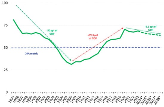
Figure 1.
African central government debt, 1995–2028 (percent of GDP). Source: Afreximbank Research, from IMF Global Debt Database. Note: “ppt” denotes percentage points and * forecast.
In all likelihood, foreign direct investment (FDI), just like debt, is an essential contributor to the infrastructure development and sustenance of economies, especially those of the developing economies of the world. It is the most stable and essential foreign source of financing, accounting for 39% of total incoming capital in developing economies (UNCTAD, 2018). According to Nowbutsing (2009), FDI can have an impact on economic growth via two major channels: the direct effect and the indirect effect. The direct effect ensures that FDI contributes to output growth by driving capital accumulation, both from the foreign investment itself and the domestic investment it stimulates, while also boosting labor demand (Makiela & Ouattara, 2018). Indirectly, FDI influences economic growth by enhancing total factor productivity through its spillover effects on domestic capital investment. Asghari et al. (2014) propose a third channel, known as the export effect. In this channel, FDI intensifies product competition in the host country, encouraging local firms to seek external markets and boosting domestic productivity. Although there has been mixed evidence across several empirical studies regarding FDI’s effect on host country economic growth, with some works in support while others are against it, effective utilization of FDI in any economy with limited barriers yields a positive growth trajectory over the long term.
Over the years, Africa has been a great beneficiary of FDI. It was estimated by the United Nations Conference on Trade and Development in its world investment report that FDI into Africa in 2022 accounted for about 3.5% of global FDI, even with a 44% decline from the previous year’s all-time high. Despite this, it can be said that it is inconclusive on the continent whether FDI actualizes its goal as a tool for financing development, facilitating technology transfer, enhancing human capital, and creating a ‘competitive effect,’ all of which promote domestic efficiency, productivity spillovers, and exports (Smarzynska, 2002; Hermes & Lensink, 2003; Adams, 2009).
1.2. Research Question and Its Significance
There is a body of economic literature that examines the history and various aspects of Africa’s public debt dynamics and FDI, as well as the challenges and shortcomings they pose for policymakers. Current economic trends on the continent and the present state of public borrowing appear to tell divergent stories. Also, the amount of Africa’s share of global FDI is an indication that Africa has traditionally lagged other regions as a destination for FDI. This brings into question whether Africa is taking advantage of the current global interconnectedness of all forms of capital by allowing for more investment transfer from the diaspora. It also needs to be understood whether there is any relationship between an economy’s public debt, its access to it, and the performance of its FDI. And finally, whether the economy’s debt capacity is optimized. That is, it is accessing the right amount of debt that will enable the actualization of sustained economic growth and development on the continent.
While most economic research examines debt and FDI linear effects on growth independently, this work will attempt to examine the two concepts’ connectedness and their implication in the African continent growth theory framework using a non-linear approach. Therefore, the objective of this study is two-faceted. One is to estimate the desirable public debt threshold level for sustainable economic growth, commonly defined as an increase in income per capita that can be maintained without an unbearable increase in public or private debt (Cecchetti et al., 2011). Secondly, we examine the influence of the public debt threshold on FDI and how it impacts the growth of African economies. We achieve this by the estimation technique that allows for a change in FDI regression coefficients (fixed effect) from one regime to another as the debt threshold changes. The consideration of FDI’s impact in this study will help bring a new perspective to this topic area, thereby serving as a premise for future economic research.
1.3. Summary of Results
The results of this literature make it evident that there is no single debt threshold range applicable to all African countries under consideration. It also attests that the debt threshold range is very sensitive to varying modeling choices. We observe a desirable minimum debt threshold of about 22% and a maximum debt threshold of about 85%. Although further research and analysis are recommended in this topic area, our results clearly suggest that a public debt-to-GDP ratio below the bottom debt threshold is associated with a negative effect on FDI growth. The robustness specifications conducted with the different control variables show that this negative effect of FDI below the minimum debt threshold is consistent across all of our analyses. Above the minimum threshold, the results of all the analyses concluded that the FDI growth effect is positive, albeit not significant for the most part. The results also show that the major control variables, such as population growth rate, human capital index, and total factor productivity, are in line with the conventional growth theory framework.
2. Literature Review
2.1. Brief Theoretical Review
John Maynard Keynes advocated for deficit financing, that is, spending more when tax revenue is low, as a method to stimulate economic activity during a recession. He argued that addressing the Great Depression required a combination of two approaches to boost the economy: increased government investment in infrastructure and lowering interest rates (Keynes, 1936). The theory promotes the combined use of both monetary and fiscal policies to stimulate economic growth. Specifically, it supports the application of expansionary fiscal policy during periods of recession to boost the economy. Conversely, when the economy is in a boom, contractionary fiscal measures are recommended to help maintain stability. When government spending exceeds its revenue, one way to finance the shortfall is by borrowing. Increasing government spending without raising taxes or cutting taxes without reducing expenditure will stimulate overall demand. However, an increase in government borrowing can lead to higher interest rates, raising the cost of borrowing for investors, which can result in a crowding-out effect. Conversely, the central bank can adjust interest rates to encourage economic activity. Lowering interest rates reduces borrowing costs for investors, leading to increased investment, while higher interest rates discourage investment and may further contract the economy.
2.2. Empirical Review
A vast amount of the empirical literature exists on the debt and FDI effects on economic growth, consisting of both linear and non-linear methodologies, since there is no single theoretical or empirical framework that fully explains the relationship between debt, FDI, and growth. A limited number of studies have focused on samples from developing countries, and even Africa.
Reinhart and Rogoff’s work, “Growth in a Time of Debt”, argues for the non-linear effects of debt on growth, suggesting that low levels of debt can stimulate growth, while excessive debt is detrimental to economic progress. Therefore, in the early stages of development, borrowing is encouraged to support productive investments. Their research utilizes a dataset covering 44 countries over 200 years, comprising more than 3700 annual observations. Their analysis shows that the relationship between government debt and real GDP growth is weak when the debt-to-GDP ratio is below 90%. However, once this threshold is exceeded, median growth rates decline by 1%, with average growth falling even more significantly. They also concluded that the public debt threshold is comparable in both advanced and emerging economies.
A critique of Reinhart and Rogoff by Herndon et al. (2014) pointed out errors attributed to coding mistakes, exclusion of data, and unusual weighting of summary statistics that resulted in significant inaccuracies in the relationship between public debt and GDP growth across 20 advanced economies in the post-war period. They henceforth concluded that the average real GDP growth rate for countries with a public-debt-to-GDP ratio over 90% is actually 2.2%, rather than the −0.1% reported by Reinhart and Rogoff. This finding suggests that, on the contrary, high debt-to-GDP ratios above 90% do not necessarily lead to markedly lower GDP growth. Additionally, they discovered that the relationship between public debt and GDP growth varies significantly across time periods and countries. Overall, their evidence challenges Reinhart and Rogoff’s assertion that debt levels above 90% of GDP consistently hinder economic growth.
A framework on public debt was proposed by Ghosh et al. (2013). It introduces the concept of ‘fiscal space,’ which refers to the gap between a country’s current debt level and its debt ceiling. In this model, enhancements in a country’s structural characteristics of economic growth increase the debt limit, enabling greater public borrowing as the economy improves. Their analysis involved a sample of 23 advanced economies from 1970 to 2007, where they found strong evidence of a non-linear relationship between the primary balance and lagged public debt, displaying characteristics of fiscal fatigue. They stated that the relationship follows a cubic pattern such that, at low debt levels, the primary balance shows little to no correlation, or a slightly negative one, with debt. As debt rises, the primary balance increases as well, but this responsiveness eventually weakens and then declines at very high debt levels. They concluded that the finding is robust across a wide range of conditioning variables and estimation techniques. By combining the empirical estimates of the primary balance reaction function with the actual or model-generated endogenous interest rates, they can estimate each country’s debt limit and corresponding fiscal space.
Elbadawi et al. (1997) use a quadratic model with fixed and random effects estimations on a sample of 99 developing countries, finding that debt’s impact on growth turns negative once debt levels exceed a 97% threshold. The work examines the impact of external debt overhang on growth and investment by determining sustainable debt ratios that align with growth revival, essential for reversing the deep economic crisis in sub-Saharan Africa. The central argument is that achieving solvency for HIPCs relies heavily on fostering growth by alleviating the debt burden, among other factors.
Omotosho et al. (2016) provided empirical evidence showing that a reverse U-shaped relationship exists between different types of public debt—total public debt as a percentage of GDP, external debt, and internal debt—and economic growth in Nigeria. The estimated threshold for total public debt is 73.7%, while external and internal debts have thresholds of 49.4% and 30.9%, respectively. A comparison of Nigeria’s external and total debt levels shows that these thresholds were surpassed prior to the 2005 debt forgiveness agreement but remained largely within limits afterward. They concluded that exceeding the estimated debt threshold levels could negatively impact economic growth.
Tran (2018) utilized a panel threshold analysis to determine debt limits for 14 emerging economies from 1999 to 2016. He revealed that non-Latin American economies are considered sustainable in the short term as long as their debt remains within the threshold range of 40% to 55% of GDP, while Latin American economies have likely encountered fiscal unsustainability, as their government debt-to-GDP ratios have exceeded the 35% threshold in recent years.
Karadam (2018) utilizes a Panel Smooth Transition Regression framework to analyze the impact of debt on growth in both advanced and developing countries. The analysis was conducted with an unbalanced panel data of 135 economies (24 industrial, 111 developing) for the period 1970–2012. The time period is divided into non-overlapping five-year intervals to examine the long-term relationship. The study reveals that the effect of public debt on growth gradually shifts from positive to negative as debt levels increase. Furthermore, the findings indicate that developing countries have a lower debt threshold compared to developed economies. In cases of high indebtedness, the negative impact of both long-term and short-term external public debt on growth becomes more pronounced and severe.
Imbs and Ranciere (2005) apply kernel estimations to 87 developing countries comprising both low- and middle-income countries, from 1969 to 2002. Two analyses were conducted. The first utilized standard growth regressions using three or five-year averages, while the second was conducted in an event study that utilizes all the available time variation. Their finding observed that debt overhang occurs when debt levels reach 55% to 60% of GDP.
Kwablah and Amoah (2022) utilized a fully modified ordinary least squares technique to examine the relationship between FDI and economic growth for 36 Sub-Saharan African countries over the period 1998 to 2016. It hypothesizes that for FDI to foster growth, the host country must have financial market development that considers fragility and economic freedom. The study’s uniqueness lies in incorporating financial market data accounting for fragility and an aggregate economic freedom score. The study shows that economic freedom and a well-developed financial market enhance FDI’s role in promoting economic growth in Sub-Saharan Africa.
Emako et al. (2022) analyze the impact of sector-specific FDI (in the primary, secondary, and tertiary sectors) on economic growth across 19 developing countries from 2005 to 2018, using a robust two-step system generalized method of moments (GMM). Control variables such as human capital, domestic investment, financial development, economic openness, labor force, and arable land were included. The study found that the growth effect of FDI is shaped by its sectoral composition in developing countries. FDI in manufacturing has a positive and statistically significant effect on economic growth, while FDI in the tertiary sector has a statistically significant negative effect. FDI in the primary sector shows a negative but negligible effect on growth. The findings suggest that attracting more FDI in manufacturing leads to greater economic growth.
Asafo-Agyei and Kodongo (2022) examine the effects of FDI and the mediating role of FDI absorptive capacity on economic growth in Sub-Saharan Africa using the threshold regression model. Their study shows that the threshold level of FDI inflows per person is around USD 44.67 per capita annually. Also, for FDI to significantly impact economic growth, countries must possess a minimum capacity to absorb its growth-enhancing benefits.
Law et al. (2021) uses dynamic panel methods to study developing countries and reports that thresholds do exist but vary substantially by context; in his broad developing-country sample, the public-debt threshold estimates are relatively high, and the negative effects of debt above the threshold are modest after careful treatment of endogeneity and instrument selection. Law’s study emphasizes that instrument choice and model parsimony matter: too many instruments or weak instrument sets can create spurious precision and misleading threshold estimates, so robustness requires tight instrument sets and multiple specification checks.
Okwoche and Makanza (2023) examine nonlinearity and threshold effects in public debt and growth, specifically in sub-Saharan Africa, using panel econometric methods suitable for threshold detection. They find evidence of threshold behavior in sub-Saharan Africa and stress heterogeneity across countries; some economies show earlier onset of adverse debt effects while others tolerate higher debt levels depending on institutional and macroeconomic circumstances. Their results reinforce the region-specific view: thresholds in Africa are not uniform and must be interpreted alongside institutional capacity and the composition of borrowing.
Kitutila (2024) focuses on 22 sub-Saharan African countries from 1990 to 2021 and uses Panel Smooth Transition Regression (PSTR) together with generalized method-of-moments robustness checks. Kitutila reports strong evidence that public debt nonlinearly affects growth and identifies a threshold beyond which debt becomes harmful to growth.
Alsamara et al. (2024) analyzes panel data for a regional sample using modern threshold frameworks (including structural/dynamic threshold regressions and Cross-Sectionally Augmented Autoregressive Distributed Lag model in some variants) and finds threshold evidence typically in the 50–60% range, depending on the sample and specification. Alsamara’s results show that public debt above the identified threshold is associated with weaker growth dynamics, but the paper also documents that short-run vs. long-run effects differ and that results are sensitive to variable selection and lag structures.
A new study by Olowofeso et al. (2023) examines the disaggregated components of public debt in the West African Monetary Zone (WAMZ) using panel threshold models and finds component-specific thresholds: for example, about 87.45% of GDP for total public debt, 12.71% for external debt, 46.94% for domestic public debt, and 17.80% for total debt service. The study provides strong empirical support for the idea that different debt components have distinct threshold levels and thus the one-size-fits-all threshold notion is flawed.
Most recently, Carrington et al. (2025) investigated debt-growth dynamics in commodity-dependent versus non-commodity-dependent developing economies using dynamic panel threshold techniques that address endogeneity. They find that commodity dependence matters: commodity-dependent countries often exhibit different (and sometimes lower) tolerable debt thresholds due to volatile revenue streams and refinancing risk; the paper documents threshold values that vary across sub-groups and again emphasizes that institutional and exposure differences are critical for interpreting any “debt cliff” notion.
From the literature review, it is clear that evidence was provided on the impact that debt and FDI have on growth, in some cases, calculating the threshold levels required for them to effectively affect economic growth. We can also observe that debt and FDI impact on growth were treated by the different authors individually, and no work was carried out to examine the connectedness of both debt and FDI on growth. This study fills this gap by incorporating FDI and debt into a single framework to ascertain their growth effect. Please note that our study is closely related to some important papers in the literature. For example, Oche et al. (2016) examined the long-run correlation between public debt and FDI in South Africa, without accounting for threshold effects. Ndoricimpa (2020) allowed for a threshold effect; however, the threshold follows a smooth transition, unlike the discrete transition in the paper.
3. Econometric Model
In order to estimate the effect of debt and the FDI effect on economic growth rate, we implement a balanced panel threshold model, which is an extension of the original Hansen’s (1999) setup by considering the long-term effect of the regressors and region-varying variable on the dependent variable. The data under consideration is a balanced panel data, yit, qit, xit; where 1 ≤ i ≤ n, 1 ≤ t ≤ N. The subscript i denotes the country, and t denotes time. The dependent variable yit is a scalar, the threshold variable qit is an unobservable scalar, and the independent variable of interest xit is a k-dimensional vector. zit includes other control variables. The model equation of interest is thus as follows:
yit = φ + β1xitI(qit ≤ λ1) + β2xitI(λ1 < qit ≤ λ2) + β3xitI(λ2 < qit) + ui + δzit + eit
The thresholds are arranged in ascending order such that λ1 < λ2, ui represents the individual effect, and I(.) is the indicator function.
Another intuitive way to express the model equation (other controls are suppressed for clarity) is as follows:
An alternative representation of the model presents
where β = (β1, β2, β3), such that the model equation can be simplified to the following:
yit = φ + βxitI(λ1, λ2) + ui + eit
The observations are separated into three “regions” based on whether the threshold variable qit is below the lower threshold λ1, in between the two thresholds (λ1, λ2), or above the upper threshold λ2. The regimes are characterized by different regression slopes, β1, β2, and β3. To identify β1, β2, and β3, the elements of xit must vary over time. Additionally, it is crucial for our analysis and methods that the threshold level is considered exogenous and does not vary with time. Our approach does not extend to cases where the threshold variable is endogenous, and alternative methods need to be developed to handle such cases. In this regard, a future extension may incorporate quasi-experimental methods, as in Chen and Choi (2025), to control for potential endogeneity biases. The error term eit is assumed to be independently and identically distributed (iid) with a mean of zero and finite variance σ2. This independent and identical distribution assumption rules out the inclusion of lagged dependent variables in xit so that there is no endogeneity problem.
To achieve the research objective, we apply Hansen’s (1999) panel threshold model based on Stata 19 and Wang (2015) to our data, a balanced panel dataset consisting of annual data for 23 selected African countries, spanning from 1995 to 2019, prior to the COVID-19 pandemic. We do not include post-2019 data due to the regular economic conditions during COVID-19. The list of countries is presented in Table 1. The selection of countries is based solely on data availability. We include 25 out of 54 African countries. They include major developing countries such as South Africa, Egypt, and Nigeria. However, the selected sample omits some of the least developed and least populous countries, such as Djibouti and Comoros. yit denotes the natural logarithm of real GDP per capita (ln_rgdp) at current prices (in USD); the annual real GDP per capita is obtained from the IMF dataset (World Economic Outlook). xit is the vector of control variables; ui represents the FDI as a percentage of GDP (fdi), which is obtained from the World Bank database. λ1 and λ2 will be estimated using the annual central government debt as a percentage of GDP (debt), obtained from the IMF dataset (World Economic Outlook). The control variables comprise annual population growth rate (n), sourced from the IMF dataset (World Economic Outlook); annual real interest rate (r) is sourced from The World Bank databank, The International Financial Statistics, Bank Al-Maghrib and Ycharts; annual inflation rate (cpi), which is obtained from The IMF dataset (World Economic Outlook), The World Bank databank, World Development Indicators and Worlddata Info; real investment/real domestic absorption (sk) and real consumption at (2017) constant prices (rconna) are obtained from The Penn World Table; human capital index (hc) is obtained from The Penn World Table and The United Nations Development Programme Human Development Report; net export (nx) and broad money as a percentage of GDP (m2) are sourced from The World Bank databank; finally, an index of agricultural total factor productivity (agtfp), sourced from The United States Department of Agriculture, Economic Research Service will be used as a proxy for total factor productivity (TFP). The variables are summarized in Table 2.

Table 1.
List of observed countries in alphabetical order from left to right column.
Table 2.
List of variables and their definition.
As shown in Figure 2, the observed economies in our model were mostly characterized by high debt burden in the late 1990s up to the early part of the new millennium, as indicated by their levels of debt-to-GDP ratio. The ensuing lower debt-to-GDP ratio following the period of high indebtedness could be attributed to the aftermath of the debt relief initiative from the World Bank to the highly indebted poor countries. Figure 3, on the other hand, shows the somewhat steadiness of the FDI for most of the observed countries’ data for the periods under observation, with the exception of the pair of Angola and Seychelles.
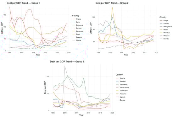
Figure 2.
Public sector debt. Source: Author’s construct from IMF dataset (World Economic Outlook). On the y-axis is the public debt as a percentage of GDP, ranging from 0% to 250%.
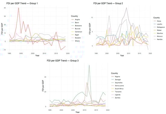
Figure 3.
Foreign direct investment. Source: Author’s construct from the World Bank database. On the y-axis is the foreign direct investment as a percentage of GDP, ranging from 0% to 60%.
Based on the data observations, it is essential to determine how public debt affects the growth sustainability of the observed economies, as well as how an economy’s debt status influences its external perception, impacting its ability to attract FDI. Ultimately, the real effect of FDI on growth can be determined through the individual effect component of the model, helping to assess whether low or high debt levels are more conducive to long-term growth. The multifaceted nature of the research question provides an indication of the incompatibility of a linear methodological approach to the study. Also, given the nature of the separated growth effects of debt and FDI that dominate most of the literature in this focus area, there is a need to evaluate growth effects from a different perspective. This perspective influenced the model choice.
4. Empirical Results
Here, we present and examine the economic significance and implications of the study’s empirical results.
4.1. Examining the Continent’s Major Economic Challenges
For our analysis, we consider some of the major economic challenges faced by the continent. Table 3 presents a simple correlation matrix of the independent variables. It shows that there is no multicollinearity.
Table 3.
Cross-correlation of some independent variables.
In view of this, we estimate our model with the independent variables consisting of inflation, population growth rate, real investment, human capital, money supply, and total factor productivity. In the regression result shown in Table 4, we observe that the desirable debt threshold level lies between 33.46% of the GDP at the lower level and 75.88% of the GDP at the upper level. Considering the FDI effect in our model, we observe that below the bottom debt threshold (region 1), a negative FDI coefficient of −0.0745 is observed. This is indicative of a negative growth effect of FDI on the economy when the debt-to-GDP ratio is lower than 33.46%. We observe this negative growth effect to be significant at 1%. An observation of the confidence interval of this negative growth effect of FDI shows that growth decline could be as much as −0.10407. At the other two debt regions, that is, in-between the two debt thresholds (region 2) and above the upper debt threshold (region 3), a positive growth effect of FDI is observed; the region 2 coefficient of FDI is very significant at 10% while the region 3 is significant only at 1%. As is evident, we observe a negative and significant (at 1%) coefficient of high population growth rate on economic growth, just like the traditional Solow model. The same negative coefficients can be said of inflation and total factor productivity, with the first not being significant while the latter is significant at 5%. This negative and significant coefficient of total factor productivity brings into question the efficiency with which production inputs are transformed into output in Africa. An observation is also made of the positive growth effect of real investment, improved human capital, and money supply on the economy, all of which are significant at 1%. Overall, our results are consistent with Reinhart and Rogoff (2010) in that debt levels can cause regime changes. In other words, our results are less in line with the conclusion of Herndon et al. (2014). However, one should note that our threshold model concerns regime-dependent impacts of FDI, not regime-dependent debt effects.
Table 4.
Public debt effect on economic growth in Africa: the FDI effect.
4.2. Robustness Checks Based on the Balanced Panel Threshold Model
Robustness checks are crucial for us to draw a conclusion based on our balanced panel threshold model. Therefore, we conduct a battery of robustness checks that include additional control variables in the model in Appendix A. They include interest rates, population, inflation, money supply, consumption, investment, and the trade balance, all of which are related to economic growth in theory.
Overall, the robustness analysis (Appendix A Table A1, Table A2, Table A3, Table A4, Table A5, Table A6 and Table A7) shows that the minimum debt-to-GDP required for sustained growth of African economies lies between 22% and 35% across a variety of models. This threshold is also identified as important for economies to continue benefiting from FDI. We observed that across all our analyses, FDI negatively impacts the economy below the minimum threshold. The negative effect of FDI on growth is also significant in most of our models. The results also conclusively show that FDI results in positive economic growth at any point above the bottom threshold. This positive growth effect is significant across all our models. The model demonstrates its robustness by providing conclusive results across all estimations. The upper threshold is established between 74% and 85%.
4.3. Robustness Checks Based on the Balanced Dynamic Panel Threshold Model
Our panel threshold model assumes that the debt variable is exogenous. However, debt levels are often endogenous to growth, as economic performance influences borrowing capacity and fiscal policy decisions. Moreover, other control variables can also be endogenous to growth, such as inflation. Therefore, we include a lagged dependent variable, lagged GDP per capita, to make our model a dynamic panel threshold model following Seo et al. (2019). We carried out GMM estimation using the Stata program developed by Seo et al. (2019); see also Caner and Hansen (2004). The program especially allows detailed diagnostics to support the threshold level.
Please note that the program allows one threshold in the debt variable due to its setup. It is in line with the findings of Reinhart and Rogoff (2010), which is the seminal paper on debt levels. In other words, we will verify whether the impacts of FDI and other macroeconomic variables depend on debt level under the conventional assumption of a single threshold.
As in Section 4.2, we consider different specifications to assess the robustness of results from the dynamic panel threshold model. Due to the mixed results, we present the following results based on a model that shows statistical significance, and keep others in Appendix A.
Table 5 shows that the debt-to-GDP threshold is estimated at 17.24%, with a highly significant bootstrap p-value indicating the presence of a non-linear relationship between debt and economic growth, thereby rejecting the null of linearity. Moreover, FDI’s impacts appear inconsistent across regimes, being negative in low-debt economies and positive in high-debt contexts. This finding is consistent with the ones based on the non-dynamic panel threshold model. Especially, the threshold is around 20% which is the lower one in the previous model that allows two thresholds.
Table 5.
Dynamic panel threshold regression results (threshold = 17.2% debt-to-GDP).
The lagged GDP variable reveals contrasting effects: a large negative coefficient in the low-debt regime and a positive, significant coefficient in the high-debt regime. Population growth exerts opposing and statistically insignificant effects. It is negative under low debt and positive under high debt, mirroring theoretical expectations that population expansion may bolster growth through labor supply in high-debt settings. The real interest rate shows a marginally positive effect in low-debt regimes and a negative effect in high-debt regimes. This appears consistent with debt overhang theory, which holds that higher interest rates attract capital in low-debt contexts but dampen growth when debt burdens are high, due to rising servicing costs.
Inflation exhibits a significant, positive effect in the low-debt regime and a negative, marginally significant effect in the high-debt regime. This finding suggests that moderate inflation can stimulate growth at low debt levels, while at high debt levels, inflationary pressures may impair macroeconomic stability and erode real incomes.
Monetary expansion presents similar regime-dependent behavior. That is, negative at low debt but positive at high debt. Thus, indicating that liquidity expansion may constrain growth when debt levels are low but become supportive under fiscal stress. The debt-to-GDP coefficient itself reveals a small positive but insignificant effect in the low-debt regime and a marginally negative effect in the high-debt regime, reinforcing the notion that moderate debt may support growth via public investment, while excessive debt tends to hinder it. The 17.24% threshold, therefore, represents a critical inflection point beyond which debt accumulation begins to offset its potential growth benefits. The Hansen’s J-test confirms instrument variable exogeneity, and the Arellano–Bond tests support the model’s specification, confirming valid moment conditions and the exogeneity of the lagged debt instrument. Overall, the results suggest that debt thresholds are much lower than traditionally observed, implying that fiscal sustainability concerns may arise earlier for some economies. Inflation and monetary policy are identified as key channels influencing growth, with effects that reverse across regimes.
Overall, the robust analysis (Table 5 and Appendix A Table A8, Table A9, Table A10, Table A11, Table A12, Table A13 and Table A14) establishes the non-linear relationship between public debt and economic growth, employing lagged dependent variable and GMM estimation. Across eight progressively specified models, the bootstrap p-value consistently rejects the null hypothesis of linearity (p = 0.000 in all cases), confirming the presence of structural breaks in growth dynamics. This finding validates the threshold framework as superior to linear specifications and aligns with theoretical expectations of regime-dependent fiscal effects. Estimated thresholds span a wide range from 17.24% in parsimonious models to 80.79% in comprehensive specifications incorporating demand-side controls, reflecting sensitivity to model structure, sample composition, and variable inclusion. Lower thresholds emerge in models with fewer regressors, suggesting that even modest debt levels can alter growth trajectories in economies with limited fiscal capacity, while higher thresholds (60–90%) appear when consumption, investment, and monetary variables are controlled, consistent with Reinhart and Rogoff’s (2010) observations of growth impediments in high-debt environments.
The analysis does not show strong support for regime-dependent impacts of FDI on the economy across eight specifications. However, the specification in Table 5 is in line with our main results.
5. Conclusions
This analysis finds evidence, using panel threshold regression on data from across 23 selected African countries from 1995 to 2019, that the desirable public debt level suitable for sustained economic growth lies between 33% and 85% of GDP. The exception is a model estimated with the absence of a money supply, where the lower threshold level is 22%. Given the importance of money within the economy, the threshold limits of 33% and 85% are likely conclusive. Our analysis also shows that this debt level is important for the economies to benefit positively from FDI. The results show that FDI has a positive growth effect at all the regions above the minimum debt threshold only, that is, in regions between the two threshold limits and above the maximum limit, and the rate of growth could be as little as 2% and as high as 8% going by the different regions’ FDI coefficients. It can also be ascertained across the entire models that the positive growth effect of FDI coefficients in these regions (2 and 3) is significant. At debt levels below the minimum threshold, evidence suggests that the economy only benefits negatively from FDI, and when the confidence interval is considered, this could extend to as much as 10% negative growth, with the negative coefficient being significant for most of our analyses.
A number of explanations can be given for the outcome of the FDI effects of public debt on growth. One such is that when the government maintains very low levels of debt, it often reflects a conservative fiscal policy that prioritizes minimal borrowing. While low debt might seem fiscally responsible, it can limit the government’s ability to finance large-scale infrastructure projects or essential public services. Infrastructure, such as transportation networks, energy grids, and telecommunications, is often financed through government borrowing, as these projects require significant upfront capital that may not be available through current revenues alone. Essential services like education, healthcare, and efficient public transportation systems improve the productivity and efficiency of the workforce and industries. Foreign investors typically seek locations where they can operate efficiently, which depends on the availability of key public resources like roads, ports, reliable electricity, skilled labor, and effective communication networks. For instance, efficient logistics and transportation systems reduce costs for companies to move goods and services. Without well-maintained roads, railways, or airports, FDI projects may face delays, higher operational costs, and reduced profitability. Also, a stable and accessible energy grid is essential for industries ranging from manufacturing to technology. Without reliable power, foreign investors may hesitate to invest in energy-intensive sectors. It can also be said that a skilled workforce is often crucial to the success of FDI, especially in sectors like technology, finance, or manufacturing. Public investments in education ensure a supply of qualified workers that can meet the demands of foreign companies. Over time, the limited ability to invest in infrastructure can stifle broader economic development. Countries with low levels of public investment may find it difficult to attract the types of FDI that drive long-term growth, such as investments in high-tech industries, manufacturing, or services. Instead, FDI may focus on short-term, low-productivity sectors, which do not contribute as significantly to sustained economic development. In this regard, the literature has been trying to identify the transmission channel of FDI. Kaur et al. (2016) and Donaubauer et al. (2016) highlight the important roles of infrastructure. Moreover, Fu (2008) and Hanafy and Marktanner (2019) show how sectoral concentration and absorptive capacity enhance the positive impact of FDI on the economy. One can see that government expenditure, which is closely related to the debt level, is linked to support for each of the factors mentioned in the literature. Therefore, we believe our threshold captures these channels indirectly.
Another explanation for the FDI effect on growth could be that when debt levels are extremely low, the government is not actively borrowing from financial markets, which can leave more capital available for private-sector borrowing and investment. While this can boost investment in the short term, the lack of a balancing mechanism, such as government borrowing to finance long-term infrastructure projects, can lead to an unregulated surge in FDI. Large FDI in an economy, particularly in real estate, natural resources, or other key industries, can drive up asset prices. For example, housing prices may skyrocket, making it unaffordable for local residents. Similarly, the price of land, resources, or even stocks in certain sectors may rise to unsustainable levels, creating asset bubbles. These bubbles can eventually burst, leading to economic instability. Also, an FDI surge can lead to over-investment in specific sectors of the economy, typically those that are highly profitable or strategically important to foreign investors. For instance, FDI may heavily target sectors like mining, manufacturing, or technology while neglecting others like agriculture or services. This creates an imbalance where certain sectors grow disproportionately while others stagnate. The resulting sectoral concentration can make the economy vulnerable to shocks in those industries and reduce diversification, which is important for long-term stability. In addition, as foreign investors flood the market, they often bring with them substantial financial resources, advanced technologies, and economies of scale, allowing them to operate more efficiently than local firms. While this can increase overall productivity in the economy, it can also lead to the crowding out of domestic businesses, particularly small and medium-sized enterprises (SMEs). These local firms may struggle to compete with well-capitalized foreign companies, leading to reduced market share, lower profits, or even business closures. The long-term effect is that local entrepreneurship and innovation may decline, weakening the domestic economic base.
These research findings provide a clear picture of the impact of public debt on African economies and the desirable threshold levels for governments in their pursuit of economic growth and development. It also highlights the effects of foreign investments on African economies, as a consequence of the pursued debt policies. This work, therefore, concludes by recommending that African countries view debt as an essential means to alleviate their economies, with a significant spillover effect for FDI, thereby dispelling the myth of “very low debt economy” policy goals. That is, more debt should be encouraged, and more importantly, ensure that public debt is geared towards the development of only essential infrastructural provisions for rapid industrialization across different economic sectors. A successful implementation of this will yield more impactful positive benefits from FDI on the continent, further helping to achieve long-term, sustained economic growth and development. This recommendation aligns with other works in the topic area, such as that of Oche et al. (2016). Lastly, one possible extension to this body of work could be performed using an empirical model based on a conditional convergence equation that links the GDP per capita growth rate to the initial income per capita level, thereby estimating how much the initial income influences the infrastructure and debt objectives pursued by policymakers in Africa. Another extension concerns addressing the potential endogeneity among FDI, public debt, and GDP growth within a single framework. For example, good economic performance may attract FDI. Moreover, high public debt can also be linked to high government expenditure for short-run economic growth. In that sense, our conclusions regarding FDI’s conditional effect on growth can also be interpreted as correlation rather than causation, which requires proper identification strategies.
Author Contributions
Conceptualization, E.O. and L.X.; methodology, E.O.; software, E.O.; validation, E.O.; formal analysis, E.O.; investigation, E.O.; resources, E.O.; data curation, E.O.; writing—original draft preparation, E.O.; writing—review and editing, E.O. and L.X.; visualization, E.O.; supervision, E.O. and L.X.; project administration, E.O. All authors have read and agreed to the published version of the manuscript.
Funding
This research received no external funding.
Data Availability Statement
Data available on request from the authors.
Acknowledgments
We want to thank the Editor, three anonymous referees, and Livio Di Matteo. Their comments greatly improved the paper, which is based on a research paper by Emmanuel Oluwafemi.
Conflicts of Interest
The authors have declared no conflict of interest.
Appendix A
Appendix A.1. The Balanced Panel Threshold Model
In order to test the robustness of the balanced panel threshold model, we make a number of alterations to the control variables in the model. At first, we estimate the model following the inclusion of the real interest rate. As shown in Table A1, we observe a similar result, indicating a desirable debt threshold level of between 33.46% and 75.88% of the GDP. Just like the result in Table 4, we observe a negative FDI effect coefficient of −0.0726 below the lower debt threshold, which is also significant at 1%. At regions 2 and 3, we observe a positive FDI growth effect, both significant at 5% and 1%, respectively. Negative coefficients are observed for population growth, inflation, total factor productivity, and real interest rate, and just like Table 4, only the inflation coefficient is observed to be insignificant at any level. We also observe positive coefficients of real investment, human capital, and money supply, with all three coefficients being significant at 5% or 1%.
Table A1.
Observing the adjustment for the interest rate.
Table A1.
Observing the adjustment for the interest rate.
| Variable | Debt | ln_rgdp | Region 1 | Region 2 | Region 3 |
|---|---|---|---|---|---|
| Threshold 1 | 33.464 | ||||
| Threshold 2 | 75.881 | ||||
| n | −0.118 *** (0.027) | ||||
| cpi | −0.000 (0.000) | ||||
| sk | 1.99 × 10⁻⁶ ** (7.88 × 10⁻⁷) | ||||
| r | −0.005 ** (0.002) | ||||
| hc | 0.881 *** (0.072) | ||||
| agtfp | −0.003 ** (0.001) | ||||
| m2 | 0.021 *** (0.001) | ||||
| fdi | −0.073 *** (0.015) | 0.019 ** (0.009) | 0.047 *** (0.007) | ||
| Constant | 6.031 *** (0.189) | 5.171 *** (0.180) | 4.665 *** (0.185) |
Standard errors in parentheses, *** p < 0.01, ** p < 0.05, * p < 0.1.
For further tests, we estimate the control variables with only population growth rate, inflation, interest rate, and money supply. We then observe that the desirable debt threshold level lies between 34.74% and 75.88% of the GDP. Also, at a lower debt level, less than 34.74% of the GDP (region 1), there is a negative growth effect of FDI on the economy with a 1% significance, while a positive effect of FDI is observed above the minimum threshold level (regions 2 and 3). This positive growth effect of FDI is observed to be significant at 5% for region 2 and at 1% for region 3. As expected, a negative effect of high population is observed on growth rate, the same can be said of real interest rate and inflation, albeit only the population growth effect is observed to be significant, at 1%. On the other hand, money supply shows a positive and a 1% significant growth effect on real GDP per capita. This result can be seen in Table A2.
Table A2.
Observing population, inflation, interest rate, and money.
Table A2.
Observing population, inflation, interest rate, and money.
| Variable | Debt | ln_rgdp | Region 1 | Region 2 | Region 3 |
|---|---|---|---|---|---|
| Threshold 1 | 34.742 | ||||
| Threshold 2 | 75.881 | ||||
| n | −0.139 *** (0.030) | ||||
| cpi | −0.000 (0.000) | ||||
| r | −0.002 (0.002) | ||||
| m2 | 0.029 *** (0.001) | ||||
| fdi | −0.060 *** (0.016) | 0.024 ** (0.011) | 0.051 *** (0.008) | ||
| Constant | 7.219 *** (0.114) | 6.250 *** (0.115) | 5.630 *** (0.126) |
Standard errors in parentheses, *** p < 0.01, ** p < 0.05, * p < 0.1.
Further estimation of the Table A2 model to include real consumption and real investment into the model maintains the desirable debt threshold for growth in the economy to be between 34.74% and 75.88% of the GDP. A negative growth effect of FDI is observed at region 1 due to the estimated negative FDI coefficient; this is observed to be significant at 1%. In regions 2 and 3, however, an observation is made of the positive FDI coefficient; a 5% significance of the FDI coefficient is observed at region 2, while region 3’s FDI coefficient is significant at 1%. Also observable is the negative population growth effect, which is significant at 1%, while real interest rate and real inflation maintained the negative effect they have on growth, albeit not significant. It can be observed that the coefficients of money, real consumption level, and real investment level impact the economy positively, with only the coefficient of money having a significance, observed at 1%. This result is presented in Table A3.
Table A3.
Controlling with real consumption and real investment.
Table A3.
Controlling with real consumption and real investment.
| Variable | Debt | ln_rgdp | Region 1 | Region 2 | Region 3 |
|---|---|---|---|---|---|
| Threshold 1 | 34.742 | ||||
| Threshold 2 | 75.881 | ||||
| n | −0.159 *** (0.030) | ||||
| cpi | −0.000 (0.000) | ||||
| r | −0.001 (0.002) | ||||
| sk | 2.07 × 10⁻⁶ (1.47 × 10⁻⁶) | ||||
| rconna | 1.03 × 10⁻⁷ (2.33 × 10⁻⁷) | ||||
| m2 | 0.027 *** (0.001) | ||||
| fdi | −0.050 *** (0.016) | 0.026 ** (0.011) | 0.052 *** (0.008) | ||
| Constant | 7.223 *** (0.113) | 6.289 *** (0.115) | 5.682 *** (0.127) |
Standard errors in parentheses, *** p < 0.01, ** p < 0.05, * p < 0.1.
In order to conduct further tests, the money supply was excluded from the Table A3 model. Table A4 shows the result of the analysis, and it is noticeable that the desirable debt level for growth of the economy lies between 34.74% and 80.87% of GDP, exhibiting a 5% upward revision at the upper threshold level. We also observe consistency in the FDI coefficient signs for the FDI effect at the three regions. In this analysis, however, the negative growth impact of FDI in region 1 is not significant, whereas the positive growth effect of FDI in regions 2 and 3 is significant at the 1% level. The signs of the control variables are maintained, positive for real investment and consumption only. We observe that only the population growth rate and the real investment coefficients are significant, both at 1%.
Table A4.
Controlling for the absence of money.
Table A4.
Controlling for the absence of money.
| Variable | Debt | ln_rgdp | Region 1 | Region 2 | Region 3 |
|---|---|---|---|---|---|
| Threshold 1 | 34.742 | ||||
| Threshold 2 | 80.874 | ||||
| n | −0.485 *** (0.034) | ||||
| cpi | −0.000 (0.000) | ||||
| r | −0.001 (0.003) | ||||
| sk | 8.22 × 10⁻⁶ *** (1.87 × 10⁻⁶) | ||||
| rconna | 2.25 × 10⁻⁷ (2.99 × 10⁻⁷) | ||||
| fdi | −0.017 (0.021) | 0.029 *** (0.010) | 0.080 *** (0.014) | ||
| Constant | 8.528 *** (0.121) | 7.956 *** (0.101) | 7.273 *** (0.131) |
Standard errors in parentheses, *** p < 0.01, ** p < 0.05, * p < 0.1.
More tests warrant the inclusion of the net export variable in Table A4 model. The analysis in Table A5 shows that, with the presence of international trade, there is a significant reduction in the lower debt threshold level, making the desirable debt per GDP for the economy range between 22.28% and 80.87%. The positive coefficient of the net export variable shows the positive growth effect that export has on the economy. However, the impact is not significant. The population growth rate and real investment coefficients remained significant in the model, both at 1%, with the former negative and the latter positive. Inflation, real interest rate, and real consumption coefficients, on the other hand, are not significant. Inflation and the real interest rate have a negative impact on growth, and the latter’s effect is positive. FDI effect below the minimum threshold (region 1) continues to be negative and not significant, with a consistency of the positive and 1% significant FDI effects in the other two regions, in line with the previous model results.
Table A5.
Controlling for the absence of money in the presence of foreign trade.
Table A5.
Controlling for the absence of money in the presence of foreign trade.
| Variable | Debt | ln_rgdp | Region 1 | Region 2 | Region 3 |
|---|---|---|---|---|---|
| Threshold 1 | 22.282 | ||||
| Threshold 2 | 80.874 | ||||
| n | −0.472 *** (0.034) | ||||
| cpi | −0.000 (0.000) | ||||
| r | −0.001 (0.003) | ||||
| sk | 9.55 × 10⁻⁶ *** (1.94 × 10⁻⁶) | ||||
| rconna | 1.36 × 10⁻⁷ (3.18 × 10⁻⁷) | ||||
| nx | 5.21 × 10⁻¹² (6.51 × 10⁻¹²) | ||||
| fdi | −0.003 (0.033) | 0.026 *** (0.010) | 0.081 *** (0.014) | ||
| Constant | 8.578 *** (0.143) | 7.979 *** (0.102) | 7.243 *** (0.132) |
Standard errors in parentheses, *** p < 0.01, ** p < 0.05, * p < 0.1.
Money supply is reintroduced into the model for further robustness tests, such that we have the Table A6 model. The result shows an upward adjustment of the desirable debt threshold level, with the lower level increasing to 34.94%, a similar level to previous estimates before the Table A5 model. The upper threshold level is estimated at 84.74%, an approximately 4% increase from the previous high. The effect of money is positive and statistically significant at the 1% level, as indicated by the money supply coefficient. It can also be observed that the net export effect, while positive, is now significant at 1%. An observation of the FDI effect shows that the negative growth effect of FDI on growth below the lower threshold is significant again, even at 5%. The FDI effects in the other two regions continue to be positive and significant at 1%. The population growth effect continues to be negative and significant, while real interest rate, inflation, real investment, and real consumption coefficients are insignificant; the latter two being positive, contrary to interest rate and inflation coefficients.
Table A6.
Controlling for the money supply in the presence of foreign trade.
Table A6.
Controlling for the money supply in the presence of foreign trade.
| Variable | Debt | ln_rgdp | Region 1 | Region 2 | Region 3 |
|---|---|---|---|---|---|
| Threshold 1 | 34.945 | ||||
| Threshold 2 | 84.741 | ||||
| n | −0.154 *** (0.030) | ||||
| cpi | −0.000 (0.000) | ||||
| r | −0.001 (0.002) | ||||
| sk | 6.77 × 10⁻⁷ (1.45 × 10⁻⁶) | ||||
| rconna | 3.55 × 10⁻⁷ (2.33 × 10⁻⁷) | ||||
| nx | 3.20 × 10⁻¹¹ *** (5.07 × 10⁻¹²) | ||||
| m2 | 0.029 *** (0.001) | ||||
| fdi | −0.038 ** (0.016) | 0.034 *** (0.008) | 0.052 *** (0.010) | ||
| Constant | 7.099 *** (0.112) | 6.234 *** (0.111) | 5.600 *** (0.126) |
Standard errors in parentheses, *** p < 0.01, ** p < 0.05, * p < 0.1.
For the final robustness check, we include all the observed control variables in our analysis. In Table A7, an observation is made of somewhat consistent debt threshold levels ranging between 34.60% and 83.75% of GDP, and of all the independent variables, only inflation and real consumption coefficients are not significant at any level. A positive coefficient is observed for the human capital index, while a negative coefficient is observed for total factor productivity. The negative coefficients for the population growth rate and real interest rate are maintained, both being significant at 1% and 5%, respectively. It can be observed that real consumption now appears to hurt growth, as can be observed by the negative coefficient of the variable. The negative FDI effect on growth below the minimum threshold is maintained, with a 1% significance. The positive growth effects in the other two regions above the minimum debt threshold remain consistent and significant at 1%.
Table A7.
Estimating all observed variables.
Table A7.
Estimating all observed variables.
| Variable | Debt | ln_rgdp | Region1 | Region2 | Region3 |
|---|---|---|---|---|---|
| Threshold 1 | 34.600 | ||||
| Threshold 2 | 83.754 | ||||
| n | −0.108 *** (0.026) | ||||
| cpi | −0.000 (0.000) | ||||
| r | −0.005 ** (0.002) | ||||
| sk | 3.22 × 10⁻⁶ ** (1.28 × 10⁻⁶) | ||||
| rconna | −2.28 × 10⁻⁷ (2.07 × 10⁻⁷) | ||||
| hc | 0.961 *** (0.071) | ||||
| agtfp | −0.004 *** (0.001) | ||||
| nx | 3.64 × 10⁻¹¹ *** (4.43 × 10⁻¹²) | ||||
| m2 | 0.022 *** (0.001) | ||||
| fdi | −0.054 *** (0.014) | 0.030 *** (0.007) | 0.041 *** (0.009) | ||
| Constant | 5.785 *** (0.183) | 5.014 *** (0.175) | 4.576 *** (0.178) |
Standard errors in parentheses, *** p < 0.01, ** p < 0.05, * p < 0.1.
In conclusion, the empirical analysis above shows that the minimum debt-to-GDP required for sustained growth in African economies lies between 22% and 35% based on a variety of models. This threshold point is also identified as important for economies to continue to benefit from FDI. We observed that across all our analyses, FDI negatively impacts the economy below the minimum threshold. The negative growth effect of FDI is also observed to be significant for most of our models. The results also conclusively show that FDI results in positive economic growth at any point above the bottom threshold. This positive growth effect is observed to be significant across all of our models. The model shows its robustness by providing conclusive results across all of the estimations conducted. The upper threshold is established between 74% and 85%.
Appendix A.2. The Balanced Dynamic Panel Threshold Model
We allow for a lagged dependent variable to address endogeneity. The first model includes population, inflation, interest rate, human capital, TFP, money supply, and FDI.
In the Table A8 model, the debt-to-GDP ratio is 80.8%, consistent with Reinhart and Rogoff’s (2010) empirical findings that high public debt levels (often 60–90%) can hinder growth due to debt overhang. Countries with debt below 80.79% operate in a regime where debt may support growth, for instance, via public investment. Those above the threshold face constraints such as higher interest rates and reduced fiscal space. The highly significant bootstrap p-value (p = 0.000) indicates a structural break in the growth dynamics, thereby rejecting the null hypothesis of a linear model. This confirms that the threshold model better captures the non-linear relationship between debt and growth. This supports theories where high debt alters the effectiveness of growth drivers like FDI and human capital. It can also be observed that FDI has a negligible impact on growth in both regimes, contrary to expectations that FDI drives growth in low-debt economies. The insignificant, albeit negative, coefficients and the large standard errors in the high-debt regime suggest that FDI is not a primary growth driver. It is also observed to have a small, insignificant positive effect. An observation is also made about the lagged GDP: at low debt-to-GDP levels, there is moderate positive persistence, consistent with growth path dependence, while a large negative coefficient is observed in the high-debt regime. Population growth is observed to have a minimal impact in low-debt regimes but a potentially large positive effect in high-debt regimes, although insignificant. Human capital is observed to have a negligible effect in low-debt regimes but a potentially massive effect in high-debt regimes, though insignificant. A small negative effect of debt on growth is observed at the lower threshold, implying that debt slightly hinders growth, consistent with crowding-out effects. At higher debt levels, however, there is little positive and significant effect. Monetary expansion can be assessed to have a slight negative effect in low-debt regimes, possibly due to inflation risks, and a positive effect in high-debt regimes. This is observed by the insignificant negative and positive effects at the lower and upper thresholds, respectively. The inflation rate, investment, and agricultural TFP effects are observed to be positively marginal, albeit insignificant at the lower threshold. At high debt levels, however, mixed effects are observed of the inflation rate, investment, and agricultural TFP, all of which are insignificant. The Hansen’s J-test result suggests valid instruments for the estimation. The Arellano–Bond Tests also support the model’s validity, confirming the instruments’ exogeneity.
Table A8.
Dynamic panel threshold regression results (threshold = 80.8% debt-to-GDP).
Table A8.
Dynamic panel threshold regression results (threshold = 80.8% debt-to-GDP).
| Variable | Low-Debt Regime (debt < 80.8%) | High-Debt Regime (debt ≥ 80.8%) | |
|---|---|---|---|
| Fdi | 0.064 (0.058) | −0.042 (0.187) | |
| L.ln_rgdp | 0.597 (3.351) | −12.357 (8.958) | |
| n | 0.037 (0.692) | 0.9690 (1.851) | |
| cpi | 0.028 (0.056) | −0.042 (0.078) | |
| sk | 0.000 (0.000) | −0.000 (0.000) | |
| hc | 1.783 (19.213) | 38.298 (34.523) | |
| agtfp | −0.016 (0.100) | −0.4089 (0.372) | |
| m2 | −0.129 (0.118) | 0.2409 (0.195) | |
| debt | −0.040 (0.063) | 0.1089 (0.072) * | |
| Constant | - | 33.188 (83.384) | |
| Threshold Estimate | 80.8% (p = 0.000) | ||
| Bootstrap p-Value | 0.000 (highly significant) | ||
| Pseudo-R-squared | 0.7272 | ||
| Hansen’s J-Test p-Value | 1.000 (from simplified GMM model) | ||
| Arellano–Bond AR(1) p-Value | 0.064 (marginally significant) | ||
| Arellano–Bond AR(2) p-Value | 0.363 (insignificant) | ||
| Observations | N = 23, T = 25 (575) | ||
| Low-Debt Obs. | ~431–460 (~75–80%) | ||
| High-Debt Obs. | ~115–144 (~20–25%) | ||
| Moment Conditions | 759 | ||
Standard errors in parentheses. *** p < 0.01, ** p < 0.05, * p < 0.2.
We then consider different sets of control variables for robustness tests and report results in six tables (Table A9, Table A10, Table A11, Table A12, Table A13 and Table A14) as follows:
Table A9.
Dynamic panel threshold regression results (threshold = 73.2% debt-to-GDP).
Table A9.
Dynamic panel threshold regression results (threshold = 73.2% debt-to-GDP).
| Variable | Low-Debt Regime (debt < 73.2%) | High-Debt Regime (debt ≥ 73.2%) | |
|---|---|---|---|
| fdi | 0.022 (0.395) | 0.082 (1.285) | |
| L.ln_rgdp | 1.054 (15.621) | −0.050 (6.425) | |
| n | −0.062 (4.445) | −0.326 (4.159) | |
| r | −0.012 (0.302) | −0.055 (0.543) | |
| cpi | 0.015 (0.035) | −0.022 (0.063) | |
| sk | −0.000 (0.000) | 0.000 (0.003) | |
| hc | −0.023 (90.633) | 0.601 (11.284) | |
| agtfp | 0.012 (0.285) | 0.036 (0.579) | |
| m2 | −0.028 (0.238) | −0.019 (0.331) | |
| debt | −0.004 (0.129) | 0.082 (0.246) | |
| Constant | - | −8.782 (21.000) | |
| Threshold Estimate | 73.2% (p = 0.797) | ||
| Bootstrap p-Value | 0.000 (highly significant) | ||
| Pseudo-R-squared | 0.727 | ||
| Hansen’s J-Test p-Value | 1.000 (from simplified GMM model) | ||
| Arellano–Bond AR(1) p-Value | 0.022 (significant) | ||
| Arellano–Bond AR(2) p-Value | 0.049 (marginally significant) | ||
| Observations | N = 23, T = 25 (575) | ||
| Low-Debt Obs. | ~402–431 (~70–75%) | ||
| High-Debt Obs. | ~144–173 (~25–30%) | ||
| Moment Conditions | 782 | ||
Standard errors in parentheses. *** p < 0.01, ** p < 0.05, * p < 0.2.
Table A10.
Dynamic panel threshold regression results (threshold = 46% debt-to-GDP).
Table A10.
Dynamic panel threshold regression results (threshold = 46% debt-to-GDP).
| Variable | Low-Debt Regime (debt < 46%) | High-Debt Regime (debt ≥ 46%) | |
|---|---|---|---|
| fdi | −0.010 (0.051) | −0.003 (0.050) | |
| L.ln_rgdp | 0.311 (0.488) | −0.161 (0.370) | |
| n | −0.078 (0.443) | 0.064 (0.540) | |
| r | −0.004 (0.014) | 0.003 (0.026) | |
| cpi | 0.017 (0.027) | −0.017 (0.026) | |
| m2 | 0.037 (0.022) * | −0.010 (0.019) | |
| debt | 0.034 (0.016) ** | −0.036 (0.025) * | |
| Constant | - | 1.910 (2.474) | |
| Threshold Estimate | 46.0% (p = 0.228) | ||
| Bootstrap p-Value | 0.000 (highly significant) | ||
| Pseudo-R-squared | 0.727 | ||
| Hansen’s J-Test p-Value | 1.000 (from simplified GMM model) | ||
| Arellano–Bond AR(1) p-Value | 0.035 (significant) | ||
| Arellano–Bond AR(2) p-Value | 0.337 (insignificant) | ||
| Observations | N = 23, T = 25 (575) | ||
| Low-Debt Obs. | ~288–347 (~50–60%) | ||
| High-Debt Obs. | ~228–287 (~25–30%) | ||
| Moment Conditions | 713 | ||
Standard errors in parentheses. *** p < 0.01, ** p < 0.05, * p < 0.2.
Table A11.
Dynamic panel threshold regression results (threshold = 80.8% debt-to-GDP).
Table A11.
Dynamic panel threshold regression results (threshold = 80.8% debt-to-GDP).
| Variable | Low-Debt Regime (debt < 80.8%) | High-Debt Regime (debt ≥ 80.8%) | |
|---|---|---|---|
| fdi | −0.012 (0.029) | 0.021 (0.064) | |
| L.ln_rgdp | 0.771 (0.168) *** | 0.221 (0.901) | |
| n | 0.192 (0.185) | −0.231 (0.207) | |
| r | −0.003 (0.005) | 0.010 (0.012) | |
| cpi | −0.009 (0.007) * | 0.010 (0.007) * | |
| sk | 0.000 (0.000) *** | −0.000 (0.000) * | |
| rconna | 0.000 (0.000) ** | 0.000 (0.000) * | |
| debt | −0.005 (0.004) * | −0.005 (0.013) | |
| Constant | - | −2.525 (7.297) | |
| Threshold Estimate | 80.8% (p = 0.000) | ||
| Bootstrap p-Value | 0.000 (highly significant) | ||
| Pseudo-R-squared | 0.727 | ||
| Hansen’s J-Test p-Value | 1.000 (from simplified GMM model) | ||
| Arellano–Bond AR(1) p-Value | 0.020 (significant) | ||
| Arellano–Bond AR(2) p-Value | 0.223 (insignificant) | ||
| Observations | N = 23, T = 25 (575) | ||
| Low-Debt Obs. | ~431–460 (~75–80%) | ||
| High-Debt Obs. | ~115–144 (~20–25%) | ||
| Moment Conditions | 736 | ||
Standard errors in parentheses. *** p < 0.01, ** p < 0.05, * p < 0.2.
Table A12.
Dynamic panel threshold regression results (threshold = 36.9% debt-to-GDP).
Table A12.
Dynamic panel threshold regression results (threshold = 36.9% debt-to-GDP).
| Variable | Low-Debt Regime (debt < 36.9%) | High-Debt Regime (debt ≥ 36.9%) | |
|---|---|---|---|
| fdi | −0.011 (0.032) | −0.012 (0.068) | |
| L.ln_rgdp | 0.241 (0.786) | 0.197 (0.438) | |
| n | −0.517 (0.549) | 0.386 (0.385) | |
| r | −0.002 (0.024) | 0.001 (0.016) | |
| cpi | −0.009 (0.034) | 0.009 (0.036) | |
| sk | 0.000 (0.000) | 0.000 (0.000) | |
| rconna | −0.000 (0.000) | 0.000 (0.000) | |
| nx | 0.000 (0.000) | −0.000 (0.000) | |
| debt | −0.007 (0.013) | −0.006 (0.013) | |
| Constant | - | −2.950 (5.885) | |
| Threshold Estimate | 36.9% (p = 0.639) | ||
| Bootstrap p-Value | 0.000 (highly significant) | ||
| Pseudo-R-squared | 0.727 | ||
| Hansen’s J-Test p-Value | 1.000 (from simplified GMM model) | ||
| Arellano–Bond AR(1) p-Value | 0.042 (significant) | ||
| Arellano–Bond AR(2) p-Value | 0.560 (insignificant) | ||
| Observations | N = 23, T = 25 (575) | ||
| Low-Debt Obs. | ~144–288 (~25–50%) | ||
| High-Debt Obs. | ~287–431 (~50–75%) | ||
| Moment Conditions | 759 | ||
Standard errors in parentheses. *** p < 0.01, ** p < 0.05, * p < 0.2.
Table A13.
Dynamic panel threshold regression results (threshold = 76.3% debt-to-GDP).
Table A13.
Dynamic panel threshold regression results (threshold = 76.3% debt-to-GDP).
| Variable | Low-Debt Regime (debt < 76.3%) | High-Debt Regime (debt ≥ 76.3%) | |
|---|---|---|---|
| fdi | −0.011 (0.033) | −0.042 (0.137) | |
| L.ln_rgdp | −0.522 (1.504) | 0.618 (8.870) | |
| n | −0.352 (0.792) | −1.052 (6.568) | |
| r | 0.025 (0.034) | −0.037 (0.084) | |
| cpi | 0.013 (0.037) | −0.014 (0.041) | |
| sk | −0.000 (0.000) | −0.000 (0.000) | |
| rconna | 0.000 (0.000) | 0.000 (0.000) | |
| nx | −0.000 (0.000) | −0.000 (0.000) | |
| m2 | −0.031 (0.162) | −0.073 (0.471) | |
| debt | −0.044 (0.080) | 0.118 (0.318) | |
| Constant | - | −12.180 (61.411) | |
| Threshold Estimate | 76.3% (p = 0.221) | ||
| Bootstrap p-Value | 0.000 (highly significant) | ||
| Pseudo-R-squared | 0.727 | ||
| Hansen’s J-Test p-Value | 1.000 (from simplified GMM model) | ||
| Arellano–Bond AR(1) p-Value | 0.001 (significant) | ||
| Arellano–Bond AR(2) p-Value | 0.065 (marginally significant) | ||
| Observations | N = 23, T = 25 (575) | ||
| Low-Debt Obs. | ~402–431 (~70–75%) | ||
| High-Debt Obs. | ~144–173 (~25–30%) | ||
| Moment Conditions | 782 | ||
Standard errors in parentheses. *** p < 0.01, ** p < 0.05, * p < 0.2.
Table A14.
Dynamic panel threshold regression results (threshold = 46.0% debt-to-GDP).
Table A14.
Dynamic panel threshold regression results (threshold = 46.0% debt-to-GDP).
| Variable | Low-Debt Regime (debt < 46.0%) | High-Debt Regime (debt ≥ 46.0%) | |
|---|---|---|---|
| fdi | 0.036 (1.124) | 0.014 (0.941) | |
| L.ln_rgdp | −0.851 (21.554) | 0.014 (3.540) | |
| n | 0.054 (3.574) | 0.403 (6.286) | |
| r | 0.020 (0.344) | 0.046 (0.258) | |
| cpi | −0.054 (1.285) | 0.058 (1.195) | |
| sk | 0.000 (0.000) | −0.000 (0.000) | |
| rconna | −0.000 (0.000) | 0.000 (0.000) | |
| agtfp | 0.038 (0.316) | −0.033 (0.375) | |
| m2 | 0.056 (0.158) | −0.004 (0.227) | |
| debt | −0.019 (0.996) | −0.026 (0.870) | |
| Constant | - | −0.721 (32.197) | |
| Threshold Estimate | 46.0% (p = 0.978) | ||
| Bootstrap p-Value | 0.000 (highly significant) | ||
| Pseudo-R-squared | 0.727 | ||
| Hansen’s J-Test p-Value | 1.000 (from simplified GMM model) | ||
| Arellano–Bond AR(1) p-Value | 0.070 (marginally significant) | ||
| Arellano–Bond AR(2) p-Value | 0.140 (insignificant) | ||
| Observations | N = 23, T = 25 (575) | ||
| Low-Debt Obs. | ~288–347 (~50–60%) | ||
| High-Debt Obs. | ~228–287 (~40–50%) | ||
| Moment Conditions | 782 | ||
Standard errors in parentheses. *** p < 0.01, ** p < 0.05, * p < 0.2.
Overall, the dynamic panel threshold regression analysis conducted above robustly establishes the non-linear relationship between public debt and economic growth. Across eight progressively specified models, the bootstrap p-value consistently rejects the null hypothesis of linearity (p = 0.000 in all cases), confirming the presence of structural breaks in growth dynamics. FDI, contrary to our main results, exerts negligible and insignificant effects across all regimes. Coefficients are small, often negative in low-debt settings and weakly positive in high-debt contexts, with large standard errors signaling instability. Diagnostic tests provide mixed but generally supportive evidence. Hansen’s J-test (p ≈ 1.000 across models) suggests instrument validity. Arellano–Bond tests confirm expected first-order serial correlation (p < 0.10) and reject second-order correlation in most specifications (p > 0.10), supporting model validity.
References
- Adams, S. (2009). Foreign direct investment, domestic investment, and economic growth in sub-Saharan Africa. Journal of Policy Modeling, 31(6), 939–949. [Google Scholar] [CrossRef]
- African Development Bank. (2021). African economic outlook 2021. African Development Bank. [Google Scholar]
- Alsamara, M., Mrabet, Z., & Mimouni, K. (2024). The threshold effects of public debt on economic growth in MENA countries: Do energy endowments matter? International Review of Economics & Finance, 89, 458–470. [Google Scholar]
- Asafo-Agyei, G., & Kodongo, O. (2022). Foreign direct investment and economic growth in sub-Saharan Africa: A nonlinear analysis. Economic Systems, 46(4), 101003. [Google Scholar] [CrossRef]
- Asghari, M., Hilmi, N., & Safa, A. (2014). FDI effects on economic growth: The role of natural resource and environmental policy. Topics in Middle Eastern and African Economies, 16(2), 85–104. [Google Scholar]
- Atta-Mensah, J., & Ibrahim, M. (2020). Explaining Africa’s debt: The journey so far and the arithmetic of the policymaker. Theoretical Economics Letters, 10, 409–441. [Google Scholar] [CrossRef]
- Caner, M., & Hansen, B. E. (2004). Instrumental variable estimation of a threshold model. Econometric Theory, 20(5), 813–843. [Google Scholar] [CrossRef]
- Carrington, S. J., Padilla, L., & Pozo, R. O. H. (2025). How much debt is too much? Debt-growth dynamics in commodity-dependent and non-commodity-dependent developing economies. International Economics, 182, 100597. [Google Scholar]
- Cecchetti, S. G., Mohanty, M. S., & Zampolli, F. (2011). The real effects of debt (pp. 1–33). Bank for International Settlements. [Google Scholar]
- Chen, Z., & Choi, C. H. (2025). Impact of free trade zones on China’s ICT products trade: A PSM-DID analysis. Asia & the Pacific Policy Studies, 12(3), e70038. [Google Scholar]
- Chudik, A., Mohaddes, K., Pesaran, M. H., & Raissi, M. (2017). Is there a debt-threshold effect on output growth? Review of Economics and Statistics, 99(1), 135–150. [Google Scholar] [CrossRef]
- Donaubauer, J., Meyer, B., & Nunnenkamp, P. (2016). Aid, infrastructure, and FDI: Assessing the transmission channel with a new index of infrastructure. World Development, 78, 230–245. [Google Scholar] [CrossRef]
- Elbadawi, I., Ndulu, B., & Ndung’u, N. (1997). Debt overhang and economic growth in sub-Saharan Africa. In Z. Iqbal, & R. Kanbur (Eds.), External finance for low-income countries (pp. 49–72). International Monetary Fund. [Google Scholar]
- Emako, E., Nuru, S., & Menza, M. (2022). The effect of foreign direct investment on economic growth in developing countries. Transnational Corporations Review, 14(4), 382–401. [Google Scholar] [CrossRef]
- Fu, X. (2008). Foreign direct investment, absorptive capacity and regional innovation capabilities: Evidence from China. Oxford Development Studies, 36(1), 89–110. [Google Scholar] [CrossRef]
- Ghosh, A. R., Kim, J. I., Mendoza, E. G., Ostry, J. D., & Qureshi, M. S. (2013). Fiscal fatigue, fiscal space and debt sustainability in advanced economies. The Economic Journal, 123(566), F4–F30. [Google Scholar] [CrossRef]
- Hanafy, S. A., & Marktanner, M. (2019). Sectoral FDI, absorptive capacity and economic growth–empirical evidence from Egyptian governorates. The Journal of International Trade & Economic Development, 28(1), 57–81. [Google Scholar]
- Hansen, B. E. (1999). Threshold effects in non-dynamic panels: Estimation, testing, and inference. Journal of Econometrics, 93, 345–368. [Google Scholar] [CrossRef]
- Hermes, N., & Lensink, R. (2003). Foreign direct investment, financial development and economic growth. Journal of Development Studies, 40(1), 142–163. [Google Scholar] [CrossRef]
- Herndon, T., Ash, M., & Pollin, R. (2014). Does high public debt consistently stifle economic growth? A critique of Reinhart and Rogoff. Cambridge Journal of Economics, 38(2), 257–279. [Google Scholar] [CrossRef]
- Imbs, J., & Ranciere, R. (2005). The overhang hangover (pp. 1–20). World Bank Policy Research Working Paper 3673. World Bank Group. [Google Scholar]
- Karadam, D. Y. (2018). An investigation of nonlinear effects of debt on growth. The Journal of Economic Asymmetries, 18, e00097. [Google Scholar] [CrossRef]
- Kaur, M., Khatua, A., & Yadav, S. S. (2016). Infrastructure development and FDI inflow to developing economies: Evidence from India. Thunderbird International Business Review, 58(6), 555–563. [Google Scholar] [CrossRef]
- Keynes, J. M. (1936). The general theory of interest, employment and money (Chapters 10, 12 and 22). Macmillan. [Google Scholar]
- Kitutila, Y. W. (2024). Estimation of the public debt threshold effects on economic growth in sub Saharan African countries. African Development Review, 36(2), 377–390. [Google Scholar] [CrossRef]
- Kwablah, E., & Amoah, A. (2022). Foreign direct investment and economic growth in sub-Saharan Africa: The complementary role of economic freedom and financial market fragility. Transnational Corporations Review, 14(2), 127–139. [Google Scholar] [CrossRef]
- Law, S. H., Ng, C. H., Kutan, A. M., & Law, Z. K. (2021). Public debt and economic growth in developing countries: Nonlinearity and threshold analysis. Economic Modelling, 98, 26–40. [Google Scholar] [CrossRef]
- Makiela, K., & Ouattara, B. (2018). Foreign direct investment and economic growth: Exploring the transmission channels. Economic Modelling, 72, 296–305. [Google Scholar] [CrossRef]
- Ndoricimpa, A. (2020). Threshold effects of public debt on economic growth in Africa: A new evidence. Journal of Economics and Development, 22(2), 187–207. [Google Scholar] [CrossRef]
- Ndung’u, N., Shimeles, A., & Manda, D. K. (2021). Growing with debt in African economies: Options, challenges and pitfalls. Journal of African Economies, 30(Suppl. S1), i3–i13. [Google Scholar] [CrossRef]
- Nowbutsing, B. M. (2009). Stock market development and economic growth: The case of Mauritius. International Business and Economics Research Journal, 8, 77–88. [Google Scholar] [CrossRef]
- Oche, M. O., Mah, G., & Mongale, I. (2016). The effects of public debt on foreign direct investment in South Africa (1983–2013): An empirical analysis. Risk Governance and Control: Financial Markets and Institutions, 6(4), 448–456. [Google Scholar] [CrossRef]
- Okwoche, P. U., & Makanza, C. S. (2023). Public debt and economic growth in sub Saharan Africa: Nonlinearity and threshold effects. Cogent Economics & Finance, 11(2), 2256125. [Google Scholar] [CrossRef]
- Olowofeso, O. E., Wadda, E. N., Adeleke, A. I., Yengbe, J. R., Cham, Y., & Kanu, T. M. (2023). Public debt growth threshold in the WAMZ: Component specific evidence. WAMI Occasional Paper Series No. 32. West African Monetary Institute (Institut Monétaire de l’Afrique de l’Ouest). [Google Scholar]
- Omotosho, B. S., Bawa, S., & Doguwa, S. I. (2016). Determining the optimal public debt threshold for Nigeria. CBN Journal of Applied Statistics, 7(2), 1–25. [Google Scholar]
- Reinhart, C. M., & Rogoff, K. S. (2010). Growth in a time of debt. American Economic Review, 100(2), 573–578. [Google Scholar] [CrossRef]
- Seo, M. H., Kim, S., & Kim, Y. J. (2019). Estimation of dynamic panel threshold model using Stata. The Stata Journal, 19(3), 685–697. [Google Scholar] [CrossRef]
- Smarzynska, B. K. (2002). Does foreign direct investment increase the productivity of domestic firms: In search of spillovers through backward linkages. Policy Research Working Paper, Series 2923. The World Bank. [Google Scholar]
- Tran, N. (2018). Debt threshold for fiscal sustainability assessment in emerging economies. Journal of Policy Modeling, 40, 375–393. [Google Scholar] [CrossRef]
- United Nations of Conference on Trade and Development. (2018). United nations of conference on trade and development. United Nations. [Google Scholar]
- Wang, Q. (2015). Fixed-effect panel threshold model using Stata. The Stata Journal, 15(1), 121–134. [Google Scholar] [CrossRef]
Disclaimer/Publisher’s Note: The statements, opinions and data contained in all publications are solely those of the individual author(s) and contributor(s) and not of MDPI and/or the editor(s). MDPI and/or the editor(s) disclaim responsibility for any injury to people or property resulting from any ideas, methods, instructions or products referred to in the content. |
© 2025 by the authors. Licensee MDPI, Basel, Switzerland. This article is an open access article distributed under the terms and conditions of the Creative Commons Attribution (CC BY) license (https://creativecommons.org/licenses/by/4.0/).