Research on Circuit Partitioning Algorithm Based on Partition Connectivity Clustering and Tabu Search

Abstract

In this paper, a circuit-partitioning method is proposed based on partition connectivity clustering and tabu search. It includes four phases: coarsening, initial partitioning, uncoarsening, and refinement. In the initial partitioning phase, the concept of partition connectivity is introduced to optimize the vertex-clustering process, which clusters vertices with high connectivity in advance to provide an optimal initial solution. In the refinement phase, an improved tabu search algorithm is proposed, which combines two flexible neighborhood search rules and a candidate solution-selection strategy based on vertex-exchange frequency to further optimize load balancing. Additionally, a random perturbation method is suggested to increase the diversity of the search space and improve both the depth and breadth of global search. The experimental results based on the ISCAS-89 and ISCAS-85 benchmark circuits show that the average cut size of the proposed circuit-partitioning method is 0.91 times that of METIS and 0.86 times that of the KL algorithm, with better performance for medium- and small-scale circuits.

1. Introduction

With the rapid development of electronic technology, circuit-partitioning algorithms have been widely applied in circuit design to divide large circuits into smaller, more manageable modules, playing a significant role in integrated circuit design, system optimization, and high-performance computing [1,2,3]. A well-designed circuit-partitioning algorithm can not only improve the efficiency and reliability of the circuit but also reduce design time and costs.

The evaluation of circuit-partitioning algorithms depends primarily on two metrics: the number of cut edges and load balancing. Many heuristic algorithms are commonly used to find approximate solutions [4,5]. For example, the spectral bisection algorithm [6] achieves high-quality partitioning by computing eigenvectors and eigenvalues, but its high computational complexity limits its feasibility for large-scale systems. The spectral multi-way partitioning algorithm [7] further refines partitioning granularity. The KL algorithm [8,9] optimizes partitioning by swapping vertices to achieve load balancing. Later, the FM algorithm [10] introduced a single-point movement strategy and a bucket list structure to significantly reduce complexity.

The rapid development of machine learning theory has led to the widespread application of intelligent computing methods in the field of circuit partitioning. These intelligent computing methods include genetic algorithms [11,12,13,14,15], particle swarm optimization algorithms [16,17], bird flock algorithms [18], and others. Thang Nguyen Bui [19] proposed an efficient local optimization graph-partitioning method based on genetic algorithms to improve the graph-search capability. Johnson and Aragon [20] proposed an intelligent partitioning model based on simulated annealing to solve the graph-partitioning problem using adaptive representations and objective functions. Jovanovic [21] proposed a solution to the maximum partitioning problem based on the ant colony algorithm, significantly optimizing the partitioning results for interconnected microgrids.

In recent years, multi-level partitioning algorithms [22,23] have gained widespread attention for their ability to improve computational efficiency when handling large-scale circuits. Some common multi-level partitioning tools include Metis [24] and hMetis [25].

Many researchers have proposed improvements to multilevel partitioning algorithms. Cong J S and Lim S K proposed a circuit-clustering method based on edge separability and applied it to multilevel circuit partitioning [26]. Li J and Behjat L [27] proposed a connectivity-based clustering algorithm and applied it to VLSI circuit partitioning. Cheng R [13] proposed a coarse partitioning algorithm based on betweenness centrality clustering. Kumar proposed the stream-based Metis partitioning method [28,29] to address computational resource limitations for ultra-large-scale circuits.

The complex network-partitioning problem is usually represented using a hypergraph model [30]. Compared to traditional undirected graphs, hypergraphs allow a single edge to connect multiple vertices. To address the partitioning problem of large-scale undirected hypergraphs, many efficient and mature hypergraph-partitioning tools have emerged, such as hmetis, Patoh, and KaHyPar [31,32,33]. In addition, some studies [34,35] have proposed improved methods based on Directed Acyclic Graphs (DAGs) within the framework of multi-level partitioning. Fiduccia et al. [36] proposed a multi-level acyclic partitioning algorithm based on the DAG partitioning model and introduced a direct k-way partitioning method. Sanders [37] proposed a local optimization algorithm combining maximum flow–minimum cut and FM strategies to improve the partitioning performance of traditional multi-level partitioning frameworks.

In circuit partitioning, graphs offer a simplified representation of circuit components and their connections, making them easier to process and analyze. In contrast, hypergraphs, which allow edges to connect multiple vertices, can increase the complexity of the partitioning problem. As a result, we focus primarily on graph-based methods.

The traditional circuit-partitioning algorithms, such as Metis, often apply random partitioning strategies in the initial phase, which risks them getting stuck in local optima, wasting computational resources. Additionally, they often focus on load balancing over minimizing the number of cut edges. For example, Metis uses equivalence swapping to achieve load balancing, but increases the number of cut edges and leads to higher circuit delay. Although it employs a greedy strategy to reduce the number of cut edges in the refinement phase, it is also prone to getting stuck in local optima.

In this paper, we propose a new circuit-partitioning method based on partition clustering and tabu search. It includes four phases: coarsening, initial partitioning, uncoarsening, and refinement. And some optimization strategies are introduced to effectively reduce the number of cut edges while maintaining load balancing. In the initial partitioning phase, an initial partitioning algorithm based on partition connectivity clustering is proposed. The algorithm introduces the concept of partition connectivity and clusters the vertices with the highest connectivity in advance. It reduces inter-partition connections, significantly decreases the number of cut edges, and provides a high-quality initial solution for the refinement phase by grouping highly related vertices into the same partition. In the refinement phase, an improved tabu search algorithm is proposed. It effectively guides the search process and continuously optimizes load balancing by using flexible neighborhood search rules and a candidate solution-selection strategy based on vertex-exchange frequency. In the improved tabu search algorithm, we also suggest a random perturbation method to enhance global search capability and avoid local optima.

The main contributions of this paper are as follows: (1) A new circuit-partitioning method is proposed. (2) An initial partitioning algorithm based on partition connectivity clustering is proposed, which clusters vertices with high connectivity in advance to provide an optimal initial solution. (3) An improved tabu search algorithm is proposed, which optimizes the search process by using flexible neighborhood search, a candidate solution-selection strategy based on vertex-exchange frequency, and a random perturbation method to enhance global search capability and avoid local optima.

2. Background Knowledge

2.1. Mathematical Description of the Circuit-Partitioning Problem

The circuit is abstracted as an undirected graph $G(V,E)$, where V denotes the set of circuit modules, and $E=\{e(v_i,v_j)\mid v_i,v_j\in V\}$ denotes the set of undirected edges representing the connections between the modules. The number of vertices in the graph G where $\left|V\right|$ denotes the set of circuit modules and $E=\{e(v_i,v_j)\mid v_i\in V,v_j\in V\}$ denotes the set of undirected edges representing the connections between the modules.

The number of vertices in graph G is denoted as $\left|V\right|=n$, with individual vertices denoted as $v_1,v_2,\cdots ,v_n$.

Each vertex $v_i$ is assigned a weight $a_i$, and the total vertex weight of the graph $G(V,E)$ is denoted as $A_G={\sum }_{i=1}^n{a}_i$. The degree of vertex $v_i$ is defined as the sum of the connection weights between $v_i$ and all other vertices, denoted as $d_i={\sum }_{j=1}^{n}e(i,j)$.

In multi-level partitioning algorithms, coarsening is an important step aimed at improving partitioning efficiency by simplifying the problem scale. The coarsening process constructs a hierarchical structure by progressively reducing the size of the graph, typically by matching nodes and merging them into smaller graphs. The weight of the merged vertex is the sum of the weights of the two merged vertices:

$$a_{(i,j)}=a_i+a_j$$

(1)

where $a_i$ and $a_j$ are the weights of vertices $v_i$ and $v_j$, respectively.

For the coarsened graph $G^{\prime }(V^{\prime },E^{\prime })$, each edge $e(v_i,v_j)$ will affect the new edge $e(v_{(i,j)},v_k)$ (where $v_{(i,j)}$ is the merged vertex and $v_k$ is any other vertex connected to $v_i$ or $v_j$). The weight of the new edge can be defined as:

$$w\left(e(v_{(i,j)},v_k)\right)=w\left(e(v_i,v_k)\right)+w\left(e(v_j,v_k)\right)$$

(2)

where $w\left(e(v_i,v_k)\right)$ and $w\left(e(v_j,v_k)\right)$ are the weights of the edges between vertices $v_i$ and $v_k$, and $v_j$ and $v_k$, respectively, in the original graph.

The coarsened graph reduces the size from the original n vertices to a smaller number $n^{\prime }$. The goal of the coarsening process is to iteratively reduce the size of the graph by selecting appropriate matchings until the graph becomes small enough to allow for finer partitioning:

$$n^{\prime }=\mathrm{floor}\left({\displaystyle \frac{n}{2}}\right)$$

(3)

where $\mathrm{floor}\left(\right)$ denotes the floor operation, meaning that after each coarsening step, the number of vertices approximately halves. The total weight of the coarsened graph $A_G^{\prime }$ is the sum of the weights of all merged vertices:

$$A_G^{\prime }=\sum _{i=1}^{n^{\prime }}{a}_i^{\prime }$$

(4)

For a circuit graph $G(V,E)$, if it is partitioned into k subgraphs $G_1(V_1,E_1)$, $G_2(V_2,E_2)$, ⋯, $G_k(V_k,E_k)$, and $V_1\cup V_2\cup \cdots \cup V_k=V$, then all the subsets are referred to as the k-way partition of graph G, denoted as $P_G^k$. In the partitioning, the total vertex weight of the subgraph $G_i(V_i,E_i)$ is $A_G^i$, and the total number of vertices is $n_i$. The edges broken by the partition are called cut edges, and the total number of these cut edges is denoted as $Cut\left(P_G^k\right)$. Thus, the objective function for searching for the minimum cut edges can be simply denoted as $\mathrm{Min}\left(Cut\left(P_G^k\right)\right)$.

A balance factor $\beta$ is introduced to ensure the load balance of each partition subset, and the following condition must be satisfied:

$$(1-\beta )·{\displaystyle \frac{A_G}{k}}<A_G^i<(1+\beta )·{\displaystyle \frac{A_G}{k}},\mathrm{where}1\le i\le k.$$

(5)

The partition connectivity is an indicator to measure the closeness of a vertex to a partition. For partition j, the connectivity of vertex v to partition j can be defined as:

$$C(v,j)=\sum _{u\in j}e(u,v)$$

(6)

Among them, $e(u,v)$ denotes the weight of the edge between vertex v and vertex u in partition j, and $u\in j$ denotes all vertices belonging to partition j. The level of vertex-to-partition connectivity reflects the relevance between vertex v and partition j. The higher the connectivity, the closer the relationship between vertex v and partition j. The definition provides an important theoretical foundation for the subsequently proposed initial partitioning algorithm and refinement algorithm.

The vertex movement gain, denoted as $g(v,n)$, refers to the change in the objective function when a vertex v from subset $G_m$ is moved to another subset $G_n$. The gain can be calculated by the following formula:

$$g(v,n)=C(v,n)-C(v,m)$$

(7)

2.2. The Basic Principles of Tabu Search Algorithm

Tabu search [38,39,40] is an intelligent optimization algorithm that combines neighborhood search with various memory strategies, and is widely recognized as an efficient optimization method for finding high-quality solutions in a short time.

The basic process of tabu search is as follows: First, initialize the solution, tabu list, and relevant parameters. Next, generate multiple candidate solutions by performing a neighborhood search starting from the current solution. Then, the algorithm selects one candidate solution based on a selection strategy as the current solution for the iteration and uses it in the next iteration. If the candidate solution is in the tabu list, the aspiration criterion is applied to determine whether to accept the solution. Finally, if the evaluation of the candidate solution is better than that of the global best solution, the global best solution is updated. By repeatedly adjusting the solution, tabu search avoids revisiting previously explored solutions, effectively converging toward the global optimum, and ultimately outputs the optimal solution.

Tabu search has several key features. First, the algorithm adapts to different optimization problems and explores the diversity of the solution space using a flexible neighborhood search strategy. Second, the tabu list mechanism effectively prevents revisiting previously explored solutions and reduces the risk of getting stuck in local optima. Third, the aspiration criterion allows tabu search to accept tabu solutions under specific conditions to enhance the diversity of the search and avoid local optima. These mechanisms give tabu search strong global optimization capabilities, making it well-suited for solving complex optimization problems.

3. The Circuit-Partitioning Algorithm Based on Partition Connectivity Clustering and Tabu Search

The main goal of circuit partitioning is to divide a complex circuit system into smaller modules, to minimize the connections between modules, and maintain load balancing.

The proposed circuit-partitioning method includes the circuit-modeling process and four core phases, which are illustrated in Figure 1:

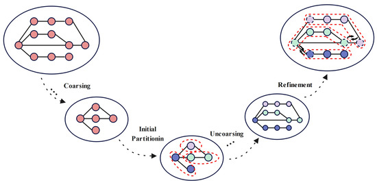
Figure 1. Flowchart of the proposed circuit-partitioning algorithm, illustrating the key stages: coarsening, initial partitioning, uncoarsening, and refinement. The vertices enclosed by the red dashed frame represent a subgraph in the partition.

Circuit Modeling: The circuit is abstracted as an undirected graph, where each electronic component is represented by a vertex, and the number of direct connections between vertices serves as the edge weights.

Coarsening phase: The circuit graph is coarsened based on Edge-Priority Matching. This coarsening process simplifies the circuit structure by merging vertices, reduces the graph’s size and complexity, and improves the efficiency of subsequent processing.

Initial Partitioning phase: The coarsened circuit graph is initially partitioned to minimize the number of cut edges while load balancing across subsets. An initial partitioning algorithm based on node-to-partition connectivity clustering is proposed to provide a good starting solution for the refinement phase.

Uncoarsening phase: This is an inverse process of the coarsening phase, and provides some exact information for the next phase, the refinement phase.

Refinement phase: The improved tabu search algorithm is used to reduce the number of cut edges generated during the initial partitioning phase. The algorithm enhances the search process by optimizing the neighborhood search rules and the candidate solution-selection mechanism based on node-exchange frequency, while the tabu list prevents redundant searches. Additionally, a perturbation method is introduced to increase the diversity of the solution space, improve global search capability, and avoid local optima. These improvements enable the improved tabu search algorithm to strike a better balance between local optimization and global exploration, ensuring load balancing and reducing cut edges, thereby optimizing the circuit-partitioning results.

3.1. Circuit Modeling and Information Storage

In digital integrated circuits, there are many types of complex connections, for example, the outputs of circuits are connected to multiple inputs, or a single output of a gate is connected to multiple inputs, etc. These connection types significantly increase the complexity of the circuit-partitioning problem. Thus, we employ graph theory to mathematically model the integrated circuits. The vertices of the graph represent the components in the circuit, while the edges represent the connections between these components. An adjacency matrix is used to collect the information of the graph, where an element corresponds to a connection. Usually, the adjacency matrix is relatively sparse and contains many zero elements. It is thus compressed and stored in the Compressed Sparse Row (CSR) format to reduce the storage requirements for large-scale circuits.

In the circuit-modeling process, the adjacency matrix M is generated by traversing all components and their connection relationships. First, all components are initially treated as vertices. For example, in Figure 2, there are seven vertices to represent the corresponding components. Next, the value of the element is set to the number of connections. If there is no connection between two components, the value of element is set to 0.

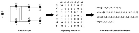
Figure 2. Transformation from a circuit graph to an adjacency matrix and compressed sparse row (CSR) matrix. The left shows the circuit graph with nodes, the middle shows the adjacency matrix, and the right shows the CSR format with xadj, adjncy, and adjwgt.

Subsequently, the adjacency matrix M is converted into the Compressed Sparse Row (CSR) storage format. The array adjncy stores the adjacent vertices for each vertex, and the related indices are stored in the array xadj, which records the starting position of each vertex’s adjacency list. The array adjwgt contains the corresponding edge weights, which represent the number of connection signals. The array vwgt contains the weight of each vertex, which represents the number of vertices.

This CSR format allows for the efficient representation and processing of the circuit’s complex structure, providing a foundation for subsequent optimization and analysis.

3.2. Coarsening Algorithm Based on Edge-Priority Matching

The coarsening techniques are widely used as a key step to simplify the original circuit graph and improve the efficiency of subsequent processing. The core operation of the coarsening process is merging two vertices into one. And the random matching or maximum weight matching methods are always used to select the merged vertices. The random matching method matches two adjacent vertices randomly, while the maximum weight matching method matches adjacent vertices with the highest edge weights to effectively reduce the number of cut edges.

Figure 3 illustrates the process of maximum weight matching. The original graph consists of eight vertices, and vertices are traversed to select the pair with the highest edge weight from adjacent vertices. The matched vertex pairs are represented by the same color. After merging the matched vertices, a coarsened graph with 20 edges is generated. The maximum weight-matching algorithm traverses vertices sequentially during the matching process, which may overlook some vertices connected by edges with higher weights. For example, in Figure 3, the edge between vertex 5 and vertex 7 has a weight of 5, which is the highest in the original graph, yet it is not matched. To address this issue, a coarsening algorithm based on edge-priority matching is proposed, as shown in Algorithm 1.

Algorithm 1 Coarsening Algorithm Based on Edge-Priority Matching

1: Input: Graph $G_1(V_1,E_1)$ with edge weights W, threshold $V_{limit}$   2: Output: Coarsened graph $G_m(V_m,E_m)$   3: Variable: Current graph $G^{\prime }(V^{\prime },E^{\prime })$, unmatched set U, matching set M (matched vertex pairs)   4: $G^{\prime }=G_1$   5: while $|V^{\prime }|>V_{limit}$ do   6:     sort edges of $G^{\prime }$ by weight (descending)   7:     $M\leftarrow \varnothing$   8:     $U\leftarrow V^{\prime }$   9:     for each edge $(u,v)$ in sorted edges do 10:         if $u\in U$ and $v\in U$ then 11:            $M.\mathrm{add}\left(\right(u,v\left)\right)$ 12:            // Remove these vertices from the unmatched set U 13:            $U.\mathrm{remove}\left(u\right)$ 14:            $U.\mathrm{remove}\left(v\right)$ 15:         end if 16:     end for 17:     Merge vertex weights by Formula (1) 18:     // Update edge weight between merged vertices and others 19:     $w\left(e(v_{(i,j)},v_k)\right)=w\left(e(v_i,v_k)\right)+w\left(e(v_j,v_k)\right)$                    // Formula (2) 20:     // Reduce the graph size by halving the number of vertices 21:     $n^{\prime }=\mathrm{floor}\left({\displaystyle \frac{n}{2}}\right)$                                                                  // Formula (3) 22:     Generate the new subgraph $G^{\prime }$ based on matched vertices and updated edge weights 23: end while 24: return $G_m(V_m,E_m)$

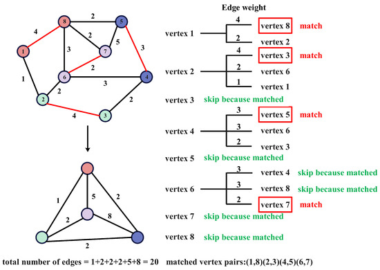
Figure 3. Illustration of the maximum weight-matching process based on vertex traversal. The graph on the left shows eight vertices connected by weighted edges. The table on the right displays the matching status for each vertex pair. The matched vertex pairs are (1,8), (2,3), (4,5), and (6,7), with a total of 20 edges in the coarsened graph.

Algorithm 1 sorts the edges of the current graph in descending order by weight. Next, it iterates through the sorted edges, attempting to match each pair of connected vertices (u, v). If both vertices are unmatched, they are added to the matching set M and removed from U to mark them as matched. After processing all edges, it generates a new coarsened graph $G^{\prime }$ using the matched set M, and updates the vertex and edge sets of the graph accordingly. This process repeats until the number of vertices in the graph is less than or equal to $V_{\mathrm{limit}}$. Finally, it returns the coarsened graph $G_m$.

An example is shown in Figure 4. The edges are first sorted by weights. Then, the vertices corresponding to the maximum weight edge, vertices 5 and 7, are matched. Next, other vertices are iteratively matched based on edge weights, resulting in a coarsened graph with 17 edges, which is a reduction of 3 edges compared to the maximum weight matching in Figure 3.

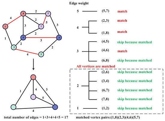
Figure 4. Illustration of an example of the coarsening algorithm based on edge-priority matching. The graph on the left shows eight vertices connected by weighted edges. The table on the right displays the matching status for each vertex pair. The matched vertex pairs are (1,8), (2,3), (4,6), and (5,7), with a total of 17 edges in the coarsened graph.

The time complexity of Algorithm 1 is primarily determined by the sorting operation, matching operation, vertex merging, edge weight updating, and the outer loop. First, in each iteration, the algorithm sorts the edges of the graph by weight. The time complexity of this sorting operation is $O\left(\right|E|log|E\left|\right)$, where $\left|E\right|$ is the number of edges in the current graph. Then, for each edge, the algorithm checks and attempts to match unmatched vertices. The time complexity of this operation is $O\left(\right|E\left|\right)$. Vertex merging and edge weight updating also require traversing all related edges, so their time complexity is also $O\left(\right|E\left|\right)$. The outer loop reduces the number of vertices by half with each coarsening operation, resulting in $O(log|V\left|\right)$ iterations, where $\left|V\right|$ is the number of vertices in the initial graph. Therefore, considering all operations, the overall time complexity is $O(log|V|·(\left|E\right|log\left|E\right|+\left|E\right|\left)\right)$.

3.3. Initial Partitioning Algorithm Based on Partition Connectivity Clustering

The coarsened graph $G_m$ was generated using Algorithm 1 in the previous section. The next step is to perform the initial partitioning. In detail, the vertices of the graph $G_m$ are assigned to k subsets $G_i$ ($G_i\in \{G_1(V_1,E_1),G_2(V_2,E_2),\dots ,G_k(V_k,E_k)\}$), ensuring that the number of vertices in each subset is as balanced as possible.

We propose an initial partitioning algorithm based on partition connectivity clustering to minimize the number of cut edges, and the main process of this algorithm is shown in Algorithm 2.

Algorithm 2 Initial Partitioning Algorithm Based on Partition Connectivity Clustering

1: Input: Input graph structure $G_m$, number of subsets k, minimum cluster weight limit $LR$   2: Output: Subgraph set S   3: Variable: Selected vertex $v_r$, a subgraph $G_i$, graph $G^{\prime }$   4: $G^{\prime }=G_m$   5: $S=\left\{\right\}$   6: for $i=1$ to k do   7:     $v_r=\mathrm{random}\mathrm{select}\left(G^{\prime }\right)$   8:     $G_i=\mathrm{ClusterSearch}(v_r,LR,G^{\prime })$   9:     $S.\mathrm{append}\left(G_i\right)$ 10:     $G^{\prime }=G^{\prime }-G_i$ 11: end for 12: return S

For each subset $G_i(V_i,E_i)$, first, a vertex $v_r$ is randomly selected as the starting point. In the subsequent steps, as described in the ClusterSearch algorithm (Algorithm 3), the partition connectivity degree in $G_m$ connected to the $G_i(V_i,E_i)$ is calculated. The vertex with the highest connectivity degree is then added to $G_i$. This process is iterated repeatedly until the weight of $G_i$ exceeds the threshold $LR$, and the ClusterSearch function returns $G_i$. Finally, $G_m$ is corrected by removing $G_i$ from it, and clustering for the next partition begins.

Algorithm 3 ClusterSearch Algorithm

1: Input: The corrected graph structure $G^{\prime }$, the minimum limit of cluster weight $LR$, and the initial vertex $v_r$   2: Output: The current subgraph $G_i(V_i,E_i)$   3: Variable: The candidate vertices set $se{t}_{vcand}$   4: $G_i.\mathrm{add}\left(v_r\right)$   5: while $G_i.\mathrm{weight}<LR$ and $se{t}_{vcand}\ne \varnothing$ do   6:     $se{t}_{vcand}.\mathrm{add}(vertices\_connected\_to\left(G_i\right))$   7:     for each vertex $v\in se{t}_{vcand}$:   8:        $C(v,i)=\mathrm{count}\_\mathrm{edges}(v,G_i)$   9:     $v_{next}=\mathrm{argmax}\left(connectivity\right)$ 10:     $G_i.\mathrm{add}\left(v_{next}\right)$ 11:     $se{t}_{vcand}.\mathrm{remove}\left(v_{next}\right)$ 12: end while 13: return$G_i(V_i,E_i)$

Figure 5 illustrates an example of Algorithm 3. Assuming vertex 2 is chosen as the initial vertex and is assigned to the starting partition $G_1=\left\{v_2\right\}$, then the adjacent vertices 1, 3, and 4 are considered as candidate vertices. Next, the partition connectivity of each candidate vertex, including $C(v_1,G_1)$, $C(v_3,G_1)$, and $C(v_4,G_1)$, is calculated as 1, 2, and 1, respectively. Therefore, vertex 3 is selected and added into the first partition; it has $G_1=\{v_2,v_3\}$.

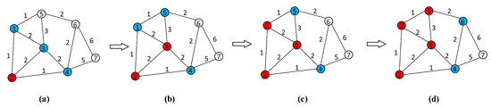
Figure 5. Example of the clustering process based on cluster connectivity priority. The red vertices represent the selected vertices, while the blue vertices represent the candidate vertices. (a) Vertex 3 is selected for $G_1=\{v_2,v_3\}$. (b) Vertex 1 is added to $G_1=\{v_1,v_2,v_3\}$ after considering edge cuts. (c) Vertex 5 is added to $G_1$. (d) Clustering stops when the threshold is exceeded.

In Figure 5b, the total partition connectivity between vertex 1 and $G_1$ is 3. Similarly, it has $C(v_5,G_1)=3$, $C(v_4,G_1)=3$. These adjacent vertices have the same partition connectivity, so the number of edge cuts is considered. In detail, clustering vertex 1 results in 7 edge cuts, clustering vertex 5 results in 9 edge cuts, and clustering vertex 4 results in 13 edge cuts. To minimize edge cuts, vertex 1 is selected and $G_1=\{v_1,v_2,v_3\}$.

In Figure 5c, the total partition connectivity between vertex 5 and $G_1$ is 4, while the total partition connectivity of vertex 4 is 3. Therefore, vertex 5 is selected.

In Figure 5d, the number of clustered vertices has exceeded the threshold, and the clustering process ends.

The time complexity of Algorithm 2 is primarily determined by the random vertex selection, the execution of the ClusterSearch function, and the outer loop. In each iteration, Algorithm 2 randomly selects a vertex and generates a subgraph through the ClusterSearch function. During the ClusterSearch process, Algorithm 2 traverses the neighboring vertices of the current subgraph and calculates the connectivity degree, selecting the vertex with the highest connectivity to add to the subgraph until the weight of the subgraph exceeds the threshold $LR$. The time complexity of the ClusterSearch function consists of operations such as updating the candidate vertex set, calculating connectivity, selecting the vertex with the maximum connectivity, and updating the subgraph. The time complexity for updating the candidate vertex set is $O\left(d\right)$, where d is the average degree of the vertices in the graph. The time complexity for calculating connectivity is $O\left(\right|E\left|\right)$, where $\left|E\right|$ is the number of edges in the graph, and selecting the vertex with the maximum connectivity has a time complexity of $O\left(\right|V\left|\right)$, where $\left|V\right|$ is the number of vertices in the graph. The operation of updating the subgraph has a time complexity of $O\left(1\right)$. Therefore, the total time complexity of the ClusterSearch function is $O\left(\right|V|·(d+\left|E\right|\left)\right)$. Since Algorithm 2 needs to execute k ClusterSearch operations, the overall time complexity is $O(k·|V|·(d+\left|E\right|\left)\right)$, where k is the number of partitions. Hence, the time complexity of Algorithm 2 is proportional to the number of vertices, edges, and partitions in the graph.

3.4. Refinement Partitioning Algorithm Based on Tabu Search

Using Algorithms 2 and 3, an initial solution is obtained. The uncoarsening process is just the inverse process of the coarsening phase. Subsequently, in the refinement phase, a tabu search algorithm is employed to optimize the number of cut edges while maintaining load balancing. Tabu search works by continuously replacing the current solution with the best neighborhood solution that has not been recently visited, thereby exploring a broader search space. The core of tabu search combines intelligent search with learning principles. It uses a flexible memory mechanism to record and leverage search history, avoiding redundant searches and improving both search efficiency and solution quality.

Building on this, we propose an effective neighborhood search strategy that explores a broader solution space through reasonable neighborhood selection to improve search quality and efficiency. We also present a perturbation method to improve its global search ability, increase the likelihood of escaping local optima, and enhance the flexibility and effectiveness of the search process.

Algorithm 4 shows the refinement process. The initial solution, current solution, candidate solution, and best solution are denoted as $P_{G_{\mathrm{init}}}^k$, $P_{G_{\mathrm{curr}}}^k$, $P_{G_{\mathrm{cand}}}^k$, and $P_{G_{\mathrm{best}}}^k$, respectively. The initial solution $P_{G_{\mathrm{init}}}^k$ is generated by the initial partitioning algorithm based on partition connectivity clustering, and its neighborhood solutions are obtained by adjusting adjacent vertices. In detail, Algorithm 4 defines two neighborhood solution-generation rules, R1 and R2, aimed at optimizing the objective (i.e., reducing cut edges) and maintaining load balancing by moving vertices in the current solution. Typically, these rules move vertices from subsets with higher weights to subsets with lower weights. Through these directed movements, the search process gradually adjusts the load balancing, bringing it closer to the ideal state. In the candidate solution-selection process, the frequency of vertex movement is applied to avoid frequently adjusting the same vertex and improve the calculation efficiency. It is noted that the new solution will only be updated as the best solution if it is at least as good as the current solution (k-partition) in terms of both the optimization objective and load balancing. Additionally, a perturbation method is suggested: if the optimal solution is not updated after $\gamma$ iterations, the current solution is perturbed to increase the possibility of escaping local optima.

Algorithm 4 Refinement Process Based on Tabu Search with a Perturbation Mechanism Algorithm

1: Input: The input graph $G_i$, initial partition $P_{G_{\mathrm{init}}}^k$   2: Output: Best partition $P_{G_{\mathrm{best}}}^k$   3: Variable: Init partition $P_{G_{\mathrm{init}}}^k$, current partition $P_{G_{\mathrm{curr}}}^k$, candidate partition $P_{G_{\mathrm{cand}}}^k$, Candidate vertex set $V_{G_{\mathrm{cand}}}$   4: Initialize iteration count, tabu list, vertex movement frequency table, and tabu tenure.   5: $P_{G_{\mathrm{best}}}^k$ = $P_{G_{\mathrm{init}}}^k$   6: for each vertex v and each subset $G_m$ do   7:     Compute move gain $g(v,m)$ by Formula (7)   8:     Place v into the bucket structure associated with $G_m$   9: end for 10: repeat 11:     // Neighborhood Solution Generation Strategy 12:     Loop through the two neighborhood generation rules $R1$ and $R2$. 13:     if turn to $R1$ then 14:         // Move a single vertex operation 15:         Select $S_m$ and vertex $v_m$ for migration 16:         Add candidate solution vertices to $V_{cand}$ according to rule $R1$. 17:     else if turn to $R2$ then 18:         // Move two vertices operation 19:         Select $S_m$ and $v_m$, then $S_n$ and $v_n$ for migration 20:         Add candidate solution vertices to $V_{cand}$ according to rule $R2$. 21:     end if 22:     // Candidate Solution Selection Strategy 23:     if turn to $R1$ then 24:         Select $v_m$ from $V_{\mathrm{cand}}$ 25:         $P_{G_{\mathrm{cand}}}^k\leftarrow P_{G_{\mathrm{curr}}}^k+\mathrm{Move}(v_m,S_m)$ 26:     else if turn to $R2$ then 27:         Select $v_m$ and $v_n$ from $V_{\mathrm{cand}}$ 28:         $P_{G_{\mathrm{cand}}}^k\leftarrow P_{G_{\mathrm{curr}}}^k+\mathrm{Move}(v_m,S_m)+\mathrm{Move}(v_n,S_n)$ 29:     end if 30:     $P_{G_{\mathrm{curr}}}^k=P_{G_{\mathrm{cand}}}^k$ 31:     Update tabu list and bucket structure 32:     // Update $P_{G_{\mathrm{best}}}^k$ 33:     if $Cut\left(P_{G_{\mathrm{curr}}}^k\right)<Cut\left(P_{G_{\mathrm{best}}}^k\right)$ or ($Cut\left(P_{G_{\mathrm{curr}}}^k\right)=Cut\left(P_{G_{\mathrm{best}}}^k\right)$ and $P_{G_{\mathrm{curr}}}^k$ is at least as balanced as $P_{G_{\mathrm{best}}}^k$) then 34:         $P_{G_{\mathrm{best}}}^k\leftarrow P_{G_{\mathrm{curr}}}^k$ 35:     end if 36:     // Perturbation mechanism 37:     if (no improvement in $P_{G_{\mathrm{curr}}}^k$ after $\gamma$ iterations) then 38:         $P_{G_{\mathrm{curr}}}^k\leftarrow \mathrm{Perturb}(P_i,p_{str})$ 39:     end if 40: until stop condition met 41: return $P_{G_{\mathrm{best}}}^k$

3.4.1. Neighborhood Solution-Generation Rule

Given a vertex v from a subset $G_m$, the gain for each other subset $G_n$ is calculated by Formula (7).

Let $P_G^k=\{G_1,G_2,\dots ,G_k\}$ be a k-way partition of the graph G, and $G_{\max }$ be the subset with the maximum weight, where $G_{\max }={max}_{i\in (1\sim k)}\left\{A_G^i\right\}$. Two neighborhood solution-generation rules are discussed as follows.

Neighborhood Solution-Generation Rule R1: Move a vertex $v_m$ with the highest gain. The specific operation is as follows: First, randomly select a subset $G_m$ ($m\ne \max$). Then, choose the vertex $v_m$ with the highest gain for subset $G_m$ from subset $G_c\in \{G_i\in P\mid A_G^i>A_G^m\}$. Finally, move the selected vertex $v_m$ to the target subset $G_m$.

Neighborhood Solution-Generation Rule R2: Move the vertex $v_m$ with the highest gain and its corresponding target subset $G_m$ according to Neighborhood Solution-Generation Rule R1. Then, randomly select another target subset $G_n\in P$, where $n\ne m$ and $n\ne \max$ (with “max” denoting the subset with the highest gain). Next, select the vertex $v_n$ with the highest gain from subset $G_c$. Finally, move $v_m$ to target subset $G_m$ and move $v_n$ to the newly selected target subset $G_n$.

R1 moves a single vertex to both optimize load balancing and reduce cut edges. It is suitable for situations where there are few cut edges but uneven load distribution, allowing for fine-grained optimization of partition quality, particularly in terms of load balancing. R1 can quickly refine the partition, avoiding unnecessary vertex movements, and is both simple and efficient in operation.

On the other hand, R2 focuses more on reducing cut edges by moving two vertices. The first vertex not only optimizes load balancing but also reduces cut edges, while the second vertex mainly serves to further reduce cut edges. R2 can significantly decrease the number of cut edges for large-scale cut edge problems. The movement of the second vertex does not need to consider load balancing, making it more focused on reducing cut edges, thereby leading to a significant reduction in the number of cut edges.

By constraining vertices to migrate from higher-weight subsets to lower-weight subsets, these neighborhood generation rules R1 and R2 gradually guide the search towards balanced partitions and reduce cut edges. They also ensure that no single subset has excessively high weight.

3.4.2. Candidate Solution-Selection Strategy

As mentioned earlier, when multiple vertices in the neighborhood solution have the same gain, a selection strategy is required to decide which vertex $v_m$ is moved to the target subset $G_m$ (and $v_n$ to $G_n$).To ensure that the selection of candidate solutions is closely tied to the current search state, the algorithm’s strategy integrates several key factors, including the tabu list and the migration frequency of vertices. The tabu list is applied to avoid the local optima or some unnecessary repeated operations, thereby maintaining diversity in the search. The migration frequency refers to the number of times a vertex has been moved during the entire search process. This information enables the algorithm to prioritize vertices that may not have been sufficiently explored or that have a more significant impact on improving the current solution.

Vertex migration is a key step in finding the optimal solution. Let $V_{\mathrm{cand}}$ denote the set of candidate vertices with the highest gain that can be moved to the target subset $G_m$. If vertex v belongs to subset $G_c$ and is in $V_{\mathrm{cand}}$, it will be migrated to $G_m$ under the following conditions:

• Vertex v is not in the tabu list;
• Moving vertex v to $G_m$ generates a new partition that improves the current best partition $P_{G_k\mathrm{best}}$.

The vertex-selection strategy utilizes two criteria to optimize the selection process. First, vertices with lower movement frequencies are prioritized to avoid frequent adjustments. This strategy can prevent repeatedly migrating the same vertices, thereby improving the diversity and efficiency of the search. Specifically, vertices with higher movement frequencies are penalized, reducing their probability of selection, thus enabling the exploration of more potential solutions.

Second, when multiple vertices in the candidate set $V_{\mathrm{cand}}$ have the same movement frequency, select those vertices that effectively balance the weight difference between the two subsets. In other words, the weight difference between the target subset and the original subset are prioritized. This approach achieves a more even distribution of load across all subsets.

3.4.3. Tabu List and Tabu Tenure Settings

Each element in the tabu list contains the following information: vertex v, original subset $G_c$, and tabu tenure t. The format is as follows: { v, $G_c$, t }, where v is the vertex being migrated, $G_c$ is the original subset containing v, and t is the tabu tenure, indicating that vertex v cannot be moved back to its original subset $G_c$ within the tabu tenure t.

$$t(v,G_c)=\left|V_{\mathrm{neig}}\left(G_c\right)\right|·\alpha +\mathrm{random}(0,2)$$

(8)

Here, $V_{\mathrm{neig}}\left(G_c\right)$ represents the number of boundary vertices relative to $G_c$, $\alpha$ is the boundary vertex ratio coefficient, and $\mathrm{random}(0,2)$ is a random integer in the range $[0,2]$.

Whenever vertex v moves from subset $G_c$ to another subset $G_m$, it is forbidden to move v back to its original subset $G_c$ for the next t iterations (the tabu period). The length of the tabu period t is dynamically adjusted based on the number of boundary vertices relative to $G_c$. This dynamic adjustment is effective in avoiding revisiting the same solution, thereby improving the diversity and efficiency of the search process.

3.4.4. Perturbation Process

If the current best partition $P_{G_k\mathrm{best}}$ has not improved after $\gamma$ iterations, a perturbation process is introduced to increase the diversity of the search. The perturbation process works by moving a selected number of $p_{\mathrm{str}}$ vertices (perturbation strength) to the specified subset.

Specifically, let the current partition be $\{G_1,G_2,\cdots ,G_k\}$, where $G_{\max }$ is the subset with the maximum vertex weight, i.e., $G_{\max }={max}_{i=1}^k\left\{A_{G_i}\right\}$. The perturbation process includes the following steps:

(1)

Randomly select a subset $G_m\in \{G_1,G_2,\cdots ,G_k\}-\left\{G_{\max }\right\}$;

(2)

Randomly select a vertex v belonging to subset $G_c$, such that $G_c\in \{G_i\in P\mid A_G^i>A_G^m\}$;

(3)

Move the selected vertex v from subset $G_c$ to subset $G_m$;

(4)

Repeat steps (1)–(3) $p_{\mathrm{str}}$ times.

Similar to the neighborhood generation rule R1, the perturbation mechanism has a key difference: it is not constrained by the tabu list and allows a vertex v to move to subset $G_m$, even if it is not a boundary vertex with respect to $G_m$. This feature enables the algorithm to escape from local optima and explore a broader solution space, thus helping to avoid being trapped in deep local optima.

3.4.5. Fast Search Method for High-Gain Vertices Based on Bucket Data Structure and Hash Table

In the circuit-partitioning problem, a vertex v is considered a “boundary vertex” only if it is adjacent to at least one vertex in subset $G_i$. Only boundary vertices may be moved to $G_i$, while moving non-boundary vertices not only has no effect but may also decrease the quality of the partition. Therefore, the algorithm’s neighborhood solution-generation strategy focuses only on boundary vertices, avoiding the consideration of all vertices. This not only improves search efficiency but also significantly reduces computational complexity.

In this paper, we propose a bucket data structure for k-way partitioning. Specifically, the algorithm maintains k bucket arrays, each corresponding to a subset. Each array contains buckets represented by doubly linked lists, where each list holds the gain and the corresponding vertex. A hash table is also used to quickly locate each vertex in the doubly linked list. This structure allows for constant-time transfers of vertices between buckets during gain updates, improving efficiency.

In the search process, the algorithm only considers boundary vertices and stores them in the bucket data structure. For each vertex v and its current subset $G_c$, the gain $g(v,m)$ can be computed in $O\left(1\right)$ time. The vertex v is only placed in the corresponding bucket if there is a vertex in $G_m$ that is adjacent to v. The gain of the vertices adjacent to v is also updated in $O\left(1\right)$ time. Therefore, the complexity of moving a vertex from one subset to the target subset depends only on the number of vertices adjacent to v. Analysis shows that k has little impact on computation time but increases memory requirements.

Figure 6 shows a schematic diagram of the bucket sorting data structure for a three-way partition of a graph with seven vertices.

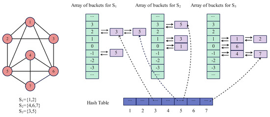
Figure 6. Illustration of the three−partition bucket sorting data structure. Seven vertices are grouped into three subsets: $G_1=\{1,2\}$, $G_2=\{4,6,7\}$, and $G_3=\{3,5\}$. The bucket array on the right stores vertices by their gain values, using linked lists for efficient updates. A hash table helps quickly locate each vertex for migration.

In Figure 6, there are 7 vertices, labeled from 1 to 7, which belong to three distinct subsets: $G_1=\{1,2\}$, $G_2=\{4,6,7\}$, and $G_3=\{3,5\}$. The right side of Figure 6 shows the corresponding bucket array structure. Each bucket array contains multiple linked lists, where each list stores vertices along with their gain information. For example, the bucket array includes buckets with different gain values such as 2, 1, 0, −1, −2, −3, and the corresponding vertices are stored in these buckets. Vertices with the same gain value are linked using a doubly linked list. The hash table facilitates the quick lookup of each vertex’s position in the doubly linked list, allowing for efficient vertex migration between buckets when updating the gain values, thereby enhancing the overall execution efficiency of the algorithm.

4. Experimental Results and Analysis

The circuit partitioning algorithm is implemented in C++ and executed on a PC with a 3.8 GHz processor, 16 GB of RAM, and the Windows 10 operating system, using a single-threaded implementation. The comparison experiments were conducted with the well-known partitioning tools METIS and some intelligent algorithms, such as genetic algorithms. The algorithm can be downloaded from https://github.com/kityAB2/circuit-partition (accessed on 5 February 2025). In the experiments, the related parameter settings are shown in Table 1, and these parameters were optimized based on results from a small number of graph-partitioning experiments.

Table 1. Parameter settings for the proposed algorithm.

Parameter	Description	Value
$V_{limit}$	Coarsening threshold	200
$LR$	Clustering weight lower bound threshold	$V/k\times (1-\beta )$
$\alpha$	Tabu list length factor	$0.1$
$P_{str}$	Perturbation strength	$0.02\times V$
$\gamma$	Number of iterations before perturbation	$0.01\times V$

All test circuits are sourced from the ISCAS-89 and ISCAS-85 benchmark datasets. The cleaned data can be downloaded from https://github.com/kityAB2/CircuitPartitioningData (accessed on 5 February 2025). The details of the number of vertices and edges in the test datasets are presented in Table 2.

Table 2. Test circuits and their vertex and edge counts.

Circuit	Number of Vertices	Number of Edges
c432	160	576
c499	202	1016
c880	383	1238
c1335	546	2200
c1908	880	3118
s1423	731	6166
s5378	2958	23,184
s9234	5808	38,053
s13207	8589	231,525
s15850	10,306	174,787
s35932	17,793	2,703,410
s38417	23,815	1,159,273

4.1. Analysis of the Two-Way Partitioning Results

4.1.1. Analysis of Minimum Edge Cut Results

The proposed algorithm is compared with the well-known partitioning tool Metis, the classic KL algorithm, and a genetic algorithm. Metis is from Karypis Lab, the KL algorithm is from reference [9], and the genetic algorithm is from reference [13]. To improve the validity of the experiments, each of the above algorithms was run 30 times, and the minimum and average cut sizes (Min and Avg) were recorded. All experiments were conducted under the condition that the balance factor $\beta$ was controlled within 0.2. The results are shown in Table 3.

Table 3. Comparison of partitioning results: Metis, KL, genetic, and proposed algorithm.

Circuit	Metis		KL [9]		Genetic [13]		Proposed
	Min	Avg	Min	Avg	Min	Avg	Min	Avg
c432	48	48	72	75	52	55	47	51
c499	57	57	85	93	66	68	48	50
c880	46	46	69	78	63	77	43	45
c1335	60	60	90	112	79	83	47	53
c1908	69	69	104	121	45	53	58	60
s1423	250	250	375	391	277	289	234	241
s5378	356	356	534	542	412	451	352	354
s9234	491	491	736	756	512	564	496	524
s13207	1429	1429	1484	1567	1797	1923	1348	1426
s15850	1468	1468	2202	2347	1436	1613	1358	1436
s35932	7232	7232	7467	7871	7119	7324	6893	6980
s38417	3286	3286	4929	5102	3541	3641	3178	3219

Figure 7 shows the comparison of the minimum cut edges between the proposed algorithm and other algorithms.

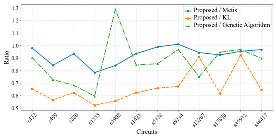
Figure 7. Ratio of proposed algorithm to other algorithms. The graph compares the ratio of the minimum values achieved by the proposed algorithm and other algorithms across the same test cases. A lower ratio indicates that the proposed algorithm performs better in optimizing the minimum cut edges compared to the other algorithms.

The experimental results demonstrate that the proposed algorithm performs excellently in circuit partitioning, overall outperforming METIS, KL algorithms, and the genetic algorithm. By comparing the minimum edge cuts (Min) and average edge cuts (Avg) of various circuits, we found that the proposed algorithm achieves optimization in most cases. Specifically, for the minimum edge cuts (Min), the proposed algorithm reaches 0.78–1.01 times that of METIS, with an average of 0.92 times; compared to KL, reaches 0.52–0.67 times, with an average of 0.62 times. As shown in Figure 7, compared to other algorithms, the ratio of the minimum cut edges is below 1 in most cases, indicating an improvement in the minimum edge cuts. However, the proposed algorithm shows weaker average stability, reflecting the variability of its results across different runs of the experiment. This phenomenon is closely related to the inherent randomness of the tabu search algorithm. The inherent randomness is effective with respect to avoiding local optima, but leads to result inconsistency. To obtain more reliable optimal results, it is recommended to execute the algorithm multiple times independently.

4.1.2. Analysis of Runtime

In the circuit-partitioning optimization problem, the running time of different algorithms is an important indicator. To evaluate the time performance of the proposed algorithm, we compared the execution times of METIS, KL algorithm, genetic algorithm, and the proposed algorithm on several circuit instances. Table 4 shows the running times on different circuits (us).

Table 4. Comparison of average execution time (µs) for different algorithms.

Circuit	Metis	KL [9]	Genetic Algorithm [13]	Proposed Algorithm
c432	1387	2412	1490	1470
c499	642	1280	1012	620
c880	1769	3806	2679	1940
c1335	2191	6250	2458	2306
c1908	3206	9251	3476	3151
s1423	2131	6200	3579	2055
s5378	7656	21,801	8740	7500
s9234	9379	27,401	14,547	9250
s13207	14,419	34,855	465,708	15,203
s15850	18,997	39,902	487,709	27,601
s35932	164,598	365,003	695,041	193,200
s38417	114,523	315,000	647,037	203,500

Compared to METIS, the average execution time of the proposed algorithm is 0.97 to 1.78 times that of METIS. On average, the execution time of the proposed algorithm is 1.13 times that of METIS, which is slightly higher, but the difference is minimal. Compared to the KL algorithm, the proposed algorithm performs better, with its execution time being 0.33 to 0.64 times that of KL. On average, the execution time of the proposed algorithm is 0.47 times that of KL, with a significant improvement in execution time, especially for medium- and small-scale circuits. Compared to the genetic algorithm, the proposed algorithm consistently exhibits lower execution times, ranging from 0.03 to 0.99 times, indicating that the proposed algorithm significantly reduces computation time in most circuits. Overall, the proposed algorithm demonstrates stable performance, with significant optimizations in execution time, especially for medium- and small-scale circuits, and outperforms both the KL algorithm and the genetic algorithm.

4.2. Analysis of Multi-Way Partitioning Results

To further evaluate the performance of the proposed algorithm, multi-way partitioning experiments were conducted with different k values (4, 8, 16). Table 5 shows the cut edge size at different k values across various circuit instances.

Table 5. Multi-way partitioning minimum results: k = 4, k = 8, k = 16.

Circuit	k = 4			k = 8			k = 16
	Metis	KL [9]	Mine	Metis	KL	Mine	Metis	KL	Mine
c432	99	121	87	136	148	117	287	304	182
c499	173	194	167	226	265	155	335	415	368
c880	119	131	97	218	226	212	337	388	279
c1335	140	157	123	254	273	231	330	421	307
c1908	119	145	110	240	241	211	604	748	571
s1423	431	476	417	518	648	405	2202	2562	2105
s5378	606	790	578	3527	4107	3186	6176	6417	5379
s9234	1025	1579	977	1414	2280	1396	4365	5067	2871
s13207	23,023	28,870	21,039	46,207	52,742	41,911	80,373	88,501	79,434
s15850	2608	3413	2414	30,642	35,816	23,361	40,760	47,213	37,469
s35932	10,644	11,744	9786	722,184	774,757	667,166	1,325,767	1,546,769	1,324,767
s38417	172,677	182,776	174,527	584,839	659,423	618,039	634,889	6,919,789	614,776

Figure 8 shows the ratio of the proposed algorithm to other algorithms in terms of the minimum cut edges for different values of k.

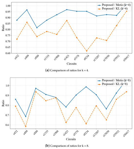
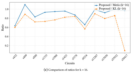
Figure 8. Comparison of ratios for different k values. This graph shows the performance comparison of the proposed algorithm and other algorithms in optimizing the minimum cut edges across different k values. A lower ratio indicates better performance of the proposed algorithm in the test cases.

The experimental results demonstrate a noticeable difference in the number of cut edges between the proposed algorithm and both METIS and KL algorithms. Compared to METIS, the proposed algorithm generally performs better, particularly for k = 4 and k = 8, where the number of cut edges is consistently lower, with the average number of cut edges being 0.91 times that of METIS. When compared to KL, the proposed algorithm also performs excellently, especially for k = 16, where the number of cut edges is significantly lower than KL, with the average being 0.86 times that of KL. Overall, the proposed algorithm shows stable performance across all test circuits, outperforming both METIS and KL in most cases, with particularly notable optimization in smaller-scale circuits.

4.3. Findings and Discussion

The circuit-partitioning optimization algorithm based on clustering and improved tabu search proposed in this study demonstrates certain advantages, particularly in reducing cut edges and optimizing load balancing. By abstracting the circuit as an undirected graph and combining clustering with the collaborative optimization of improved tabu search, we are able to effectively reduce the number of cut edges and improve the quality of partitioning. The experimental results show that the proposed algorithm performs better than traditional algorithms, such as Metis and KL, especially when handling large-scale circuits.

Compared to Metis, the proposed algorithm offers several key improvements. Metis typically requires re-optimization after each uncoarsing step, leading to increased computational complexity and time consumption. In contrast, our algorithm performs further optimization directly after uncoarsing, eliminating the need for repeated optimization steps. This approach reduces the time overhead associated with multiple optimization iterations and enhances overall computational efficiency.

Moreover, during the tabu search phase, our algorithm utilizes bucket data structures and hash tables, which significantly speed up the computation process. While Metis may require considerable time for the initial partitioning, our algorithm, thanks to its optimized data structures and design, can complete the tabu search phase more quickly. This advantage becomes especially apparent when handling large-scale circuits, where our approach outperforms traditional methods in both execution time and computational load.

The improved tabu search algorithm, through its innovative perturbation mechanism and high-quality neighborhood search, is able to converge to better solutions relatively quickly, demonstrating reasonable single-thread optimization capabilities. Although the algorithm is executed in a single-thread environment, its efficient neighborhood search and perturbation strategy allow it to find better solutions in a relatively short time, exhibiting a reasonable level of computational efficiency. In a single-threaded environment, the algorithm effectively shortens computation time, and as the scale of the circuit increases, its computational efficiency remains within a reasonable range, showing a certain degree of scalability.

In particular, when dealing with large-scale circuits, the tabu search algorithm refines the initial partitioning results, further reducing the number of cut edges while maintaining a good load balance. Even when faced with circuits containing a large number of nodes and edges, the algorithm remains stable and effective. While this is a single-threaded algorithm, its rapid convergence and efficient search process allow it to handle larger-scale circuits, demonstrating strong adaptability in practical applications.

When compared with Metis and KL algorithms, our algorithm outperforms them in reducing the number of cut edges, and even as the circuit scale increases, the optimization results remain stable and the computational time increases insignificantly. This indicates that the algorithm exhibits strong scalability in a single-threaded environment and can handle circuit partitioning tasks of varying scales and complexities.

However, when dealing with extremely complex and irregular circuit structures, the initial partition may not always find the optimal solution, limiting the optimization potential of the subsequent refinement process. Future research could further optimize the perturbation mechanism and neighborhood search strategy of the tabu search algorithm to enhance its accuracy and stability. Additionally, although the current algorithm is implemented in a single thread, future efforts could explore improving the algorithm’s ability to handle large-scale circuit optimization tasks through optimization of the algorithm itself and efficient scheduling strategies.

Overall, the circuit partitioning optimization algorithm based on partition connectivity clustering and improved tabu search demonstrates good optimization effects in reducing cut edges and enhancing load balancing. Although the current algorithm is single-threaded, its stability and efficiency in scaling up circuits make it highly applicable, providing potential directions for further optimization and expansion in the future.

5. Conclusions

The circuit-partitioning algorithm proposed in this study demonstrates significant advantages in circuit-partitioning tasks, particularly excelling in minimizing cut edges. Compared to the widely used partitioning tools METIS and KL algorithms, the proposed algorithm shows substantial improvements in minimizing cut edges across multiple circuit instances. Specifically, in terms of the minimum cut edges, the proposed algorithm generally performs better than METIS in the cases of k = 4 and k = 8, with an average of 0.91 times the cut edges of METIS. In the case of k = 16, the proposed algorithm significantly outperforms KL in cut edges, with the average cut edges being 0.86 times that of KL. Additionally, the minimum connection numbers of the proposed algorithm are 0.65 times the minimum of METIS, with the highest being 0.98 times. In terms of average connection numbers, the proposed algorithm performs better than METIS and KL, with an average of 0.92 times that of METIS and 0.84 times that of KL. Despite the significant optimization performance, the proposed algorithm also shows a certain level of competitiveness in execution time, especially when handling medium- and small-scale circuits.

In conclusion, the tabu search algorithm shows considerable potential in the field of circuit partitioning, particularly in optimizing cut edges and connection numbers. It is suitable for optimizing medium- and small-scale circuits. Future research should focus on improving the algorithm’s structure and strategies to enhance its efficiency and stability, thereby improving its applicability and reliability in large-scale circuit-partitioning tasks.

References

- Shanavas, I.H.; Gnanamurthy, R.K. Optimal Solution for VLSI Physical Design Automation Using Hybrid Genetic Algorithm. Math. Probl. Eng. 2014, 2014, 809642. [Google Scholar] [CrossRef]
- Qiu, Y.H.; Xing, Y.; Zheng, X.; Gao, P.; Cai, S.T.; Xiong, X.M. Progress of Placement Optimization for Accelerating VLSI Physical Design. Electronics 2023, 12, 337. [Google Scholar] [CrossRef]
- Nath, S.; Sing, J.K.; Sarkar, S.K. Wire length optimization of VLSI circuits using IWO algorithm and its hybrid. Circuit World 2024, 50, 205–216. [Google Scholar] [CrossRef]
- Tatsumura, K.; Hidaka, R.; Nakayama, J.; Kashimata, T.; Yamasaki, M. Real-Time Trading System Based on Selections of Potentially Profitable, Uncorrelated, and Balanced Stocks by NP-Hard Combinatorial Optimization. IEEE Access 2023, 11, 120023–120033. [Google Scholar] [CrossRef]
- Daliri, A.; Alimoradi, M.; Zabihimayvan, M.; Sadeghi, R. World Hyper-Heuristic: A Novel Reinforcement Learning Approach for Dynamic Exploration and Exploitation. Expert Syst. Appl. 2024, 244, 122931. [Google Scholar] [CrossRef]
- Rahman, A.; Liu, X.; Kong, F. A Survey on Geographic Load Balancing Based Data Center Power Management in the Smart Grid Environment. IEEE Commun. Surv. Tutor. 2014, 16, 214–233. [Google Scholar] [CrossRef]
- Zenia, N.Z.; Aseeri, M.; Ahmed, M.R.; Chowdhury, Z.I.; Shamim Kaiser, M. Energy-efficiency and reliability in MAC and routing protocols for underwater wireless sensor network: A survey. J. Netw. Comput. Appl. 2016, 71, 72–85. [Google Scholar] [CrossRef]
- Sahu, P.K.; Manna, K.; Shah, N. Extending Kernighan–Lin partitioning heuristic for application mapping onto Network-on-Chip. J. Syst. Archit. 2014, 60, 562–578. [Google Scholar] [CrossRef]
- Lei, X.; Liang, W.; Li, K.C.; Luo, H.; Hu, J.; Cai, J.; Li, Y. A New Multilevel Circuit Partitioning Algorithm Based on the Improved KL Algorithm. In Proceedings of the 2019 IEEE 5th Intl Conference on Big Data Security on Cloud (BigDataSecurity), IEEE Intl Conference on High Performance and Smart Computing, (HPSC) and IEEE Intl Conference on Intelligent Data and Security (IDS), Washington, DC, USA, 27–29 May 2019; pp. 178–182. [Google Scholar]
- Zhu, W.X.; Cheng, H. Scatter Search Algorithm for VLSI Circuit Partitioning. Acta Electron. Sin. 2012, 40, 1207–1212. [Google Scholar]
- Kim, Y.H.; Yoon, Y.; Geem, Z.W. A comparison study of harmony search and genetic algorithm for the max-cut problem. Swarm Evol. Comput. 2019, 44, 130–135. [Google Scholar] [CrossRef]
- Zhai, Q.; He, Y.; Wang, G.; Hao, X. A General Approach to Solving Hardware and Software Partitioning Problem Based on Evolutionary Algorithms. Adv. Eng. Softw. 2021, 159, 102998. [Google Scholar] [CrossRef]
- Cheng, R.; Yin, L.Z.; Jiang, Z.H.; Xu, X.M. Gate-level circuit-partitioning algorithm based on clustering and an improved genetic algorithm. Entropy 2023, 25, 597. [Google Scholar] [CrossRef] [PubMed]
- Su, Y.; Zhou, K.; Zhang, X.; Cheng, R.; Zheng, C. A parallel multi-objective evolutionary algorithm for community detection in large-scale complex networks. Inf. Sci. 2021, 576, 374–392. [Google Scholar] [CrossRef]
- Dong, Y.; Cao, L.; Zuo, K. Genetic Algorithm Based on a New Similarity for Probabilistic Transformation of Belief Functions. Entropy 2022, 24, 1680. [Google Scholar] [CrossRef] [PubMed]
- Guo, W.Z.; Chen, G.L.; Xiong, N.X.; Peng, S.J. Hybrid particle swarm optimization algorithm for VLSI circuit partitioning. J. Softw. 2011, 22, 833–842. [Google Scholar] [CrossRef]
- Wu, L.; Qu, J.; Shi, H.; Li, P. Node Deployment Optimization for Wireless Sensor Networks Based on Virtual Force-Directed Particle Swarm Optimization Algorithm and Evidence Theory. Entropy 2022, 24, 1637. [Google Scholar] [CrossRef]
- Guru, R.P.; Vaithianathan, V. An efficient VLSI circuit-partitioning algorithm based on satin bowerbird optimization (SBO). J. Comput. Electron. 2020, 19, 1232–1248. [Google Scholar] [CrossRef]
- Holland, J.H. Genetic algorithms. Sci. Am. 1992, 267, 66–73. [Google Scholar] [CrossRef]
- Rutenbar, R.A. Simulated annealing algorithms: An overview. IEEE Circuits Devices Mag. 1989, 5, 19–26. [Google Scholar] [CrossRef]
- Blum, C. Ant colony optimization: Introduction and recent trends. Phys. Life Rev. 2005, 2, 353–373. [Google Scholar] [CrossRef]
- Li, X.; Pang, Y.; Zhao, C.; Liu, Y.; Dong, Q. A New Multi-Level Algorithm for Balanced Partition Problem on Large Scale Directed Graphs. Adv. Aerodyn. 2021, 3, 23. [Google Scholar] [CrossRef]
- Trifunović, A.; Knottenbelt, W. Parallel multilevel algorithms for hypergraph partitioning. J. Parallel Distrib. Comput. 2008, 68, 563–581. [Google Scholar] [CrossRef]
- Karypis, G.; Kumar, V. METIS—Unstructured Graph Partitioning and Sparse Matrix Ordering System, Version 2.0. Appl. Phys. Lett. 2010, 97, 124101. [Google Scholar]
- Karypis, G.; Aggarwal, R.; Kumar, V. Multilevel hypergraph partitioning: Application in VLSI domain. In Proceedings of the 34th Annual Design Automation Conference, New York, NY, USA, 13 June 1997; pp. 526–529. [Google Scholar]
- Cong, J.S.; Lim, S.K. Edge separability-based circuit clustering with application to multilevel circuit partitioning. IEEE Trans.-Comput.-Aided Des. Integr. Circuits Syst. 2006, 23, 346–357. [Google Scholar] [CrossRef]
- Li, J.; Behjat, L. A connectivity-based clustering algorithm with application to VLSI circuit partitioning. IEEE Trans. Circuits Syst. II Express Briefs 2006, 53, 384–388. [Google Scholar]
- Kumar, R.; Caverlee, J.; Tong, H. Streaming METIS Partitioning. In Proceedings of the 8th IEEE/ACM International Conference on Advances in Social Networks Analysis and Mining (ASONAM), San Francisco, CA, USA, 18–21 August 2016; pp. 17–24. [Google Scholar]
- He, T.X.; Xiao, Z.; Chen, C.; Liu, C.B.; Li, K.L. DAG Partition Algorithm for Hardware Accelerated Function Verification. J. Softw. 2022, 33, 3236–3248. [Google Scholar]
- Zhao, S.; Dai, X.; Bate, I.; Burns, A.; Chang, W. DAG Scheduling and Analysis on Multiprocessor Systems: Exploitation of Parallelism and Dependency. In Proceedings of the 2020 IEEE Real-Time Systems Symposium (RTSS), Houston, TX, USA, 1–4 December 2020; pp. 128–140. [Google Scholar]
- Gottesbüren, L.; Heuer, T.; Maas, N.; Sanders, P.; Schlag, S. Scalable High-Quality Hypergraph Partitioning. ACM Trans. Algorithms 2024, 20, 1–54. [Google Scholar] [CrossRef]
- Bustany, I.; Kahng, A.B.; Koutis, I.; Pramanik, B.; Wang, Z. K-SpecPart: Supervised Embedding Algorithms and Cut Overlay for Improved Hypergraph Partitioning. IEEE Trans. Comput.-Aided Des. Integr. Circuits Syst. 2024, 43, 1232–1245. [Google Scholar] [CrossRef]
- Schlag, S.; Heuer, T.; Gottesbüren, L.; Akhremtsev, Y.; Schulz, C.; Sanders, P. High-Quality Hypergraph Partitioning. ACM J. Exp. Algorithmics 2023, 27, 1–39. [Google Scholar] [CrossRef]
- Herrmann, J.; Ozkaya, M.Y.; Uçar, B.; Kaya, K.; Çatalyürek, U.V. Multilevel algorithms for acyclic partitioning of directed acyclic graphs. Siam J. Sci. Comput. 2019, 41, A2117–A2145. [Google Scholar] [CrossRef]
- Moreira, O.; Popp, M.; Schulz, C. Evolutionary multi-level acyclic graph partitioning. In Proceedings of the Genetic and Evolutionary Computation Conference, Kyoto, Japan, 15–19 July 2018; pp. 332–339. [Google Scholar]
- Fiduccia, C.M.; Mattheyses, R.M. A linear-time heuristic for improving network partitions. In Papers on Twenty-Five Years of Electronic Design Automation; Association for Computing Machinery: New York, NY, USA, 1988; pp. 241–247. [Google Scholar]
- Sanders, P.; Schulz, C. Engineering Multilevel Graph Partitioning Algorithms. In Algorithms—ESA 2011: 19th Annual European Symposium; Springer: Berlin/Heidelberg, Germany, 2011; pp. 469–480. [Google Scholar]
- Niroumandrad, N.; Lahrichi, N.; Lodi, A. Learning tabu search algorithms: A scheduling application. Comput. Oper. Res. 2024, 170, 106751. [Google Scholar] [CrossRef]
- Ru, S.Y. Vehicle logistics intermodal route optimization based on Tabu search algorithm. Sci. Rep. 2024, 14, 11859. [Google Scholar] [CrossRef] [PubMed]
- Zhang, Q.Y.; Lu, Z.P.; Su, Z.; Li, C.M. A vertex weighting-based double-tabu search algorithm for the classical ppp-center problem. Comput. Oper. Res. 2023, 160, 106373. [Google Scholar] [CrossRef]
Disclaimer/Publisher’s Note: The statements, opinions and data contained in all publications are solely those of the individual author(s) and contributor(s) and not of MDPI and/or the editor(s). MDPI and/or the editor(s) disclaim responsibility for any injury to people or property resulting from any ideas, methods, instructions or products referred to in the content. |
© 2025 by the authors. Licensee MDPI, Basel, Switzerland. This article is an open access article distributed under the terms and conditions of the Creative Commons Attribution (CC BY) license (https://creativecommons.org/licenses/by/4.0/).