Bridging Heterogeneous Agents: A Neuro-Symbolic Knowledge Transfer Approach

Abstract

This paper presents a neuro-symbolic approach for constructing distributed knowledge graphs to facilitate cooperation through communication among spatially proximate agents. We develop a graph autoencoder (GAE) that learns rich representations from heterogeneous modalities. The method employs density-adaptive k-nearest neighbor (k-NN) construction with Gabriel pruning to build the proximity graphs that balance local density awareness with geometric consistency. When the agents enter the bridging zone, their individual knowledge graphs are aggregated into hypergraphs using a construction algorithm, for which we derive the theoretical bounds on the minimum number of hyperedges required for connectivity under arity and locality constraints. We evaluate the approach in PettingZoo’s communication-oriented environment, observing improvements of approximately 10% in episode rewards and up to 40% in individual agent rewards compared to Deep Q-Network (DQN) baselines, while maintaining comparable policy loss values. The explicit graph structures may offer interpretability benefits for applications requiring auditability. This work explores how structured knowledge representations can support cooperation in distributed multi-agent systems with heterogeneous observations.

1. Introduction

The Internet of Agents (IoA) has successfully evolved from the fusion of Internet of Things (IoT) and AI techniques [1,2]. It is plausible to argue [3,4] that one of the key paradigms for modeling and implementing many IoT scenarios is the concept of multi-agent systems (MASs), which treat every device as an agent with its own distinct set of needs, capabilities, and inter-agent relationships. An MAS provides developers with approaches that enable the design of scalable and fault-tolerant IoA systems.

On the one hand, a variety of game theoretic methods decompose multi-agent interactions into sequences of two-player zero-sum games. These methods have evolved to incorporate accurate opponent intention recognition models [5] and sophisticated state-pruning techniques, enabling faster convergence to equilibria [6], which appears to be beneficial in defense strategies and adversarial robustness analysis. On the other hand, Multi-Agent Reinforcement Learning (MARL) [7,8] enables multiple agents to simultaneously engage in general-sum games within a shared environment. Each agent receives observations, executes actions, and obtains rewards—positive signals that guide learning. Optimizing cumulative rewards across agents directly improves system-level performance metrics such as latency reduction, task completion rates, and resource efficiency, which serves to advance practical multi-agent systems in domains ranging from autonomous logistics to distributed sensing networks.

A central challenge in MARL is learning to cooperate within non-stationary environments and with limited local information [9,10,11]. The centralized training with decentralized execution (CTDE) paradigm partially mitigates non-stationarity by exploiting global signals during training while relying on local observations during execution [12,13,14]. However, most CTDE approaches assume fixed communication routes, manually designed message structures or implicit weight exchange, which restricts scalability and interpretability.

Over the past few years, researchers have proposed differentiable communication architectures to improve coordination, including CommNet [15], DIAL [16], TarMAC [17], and more recent transformer- and graph-based models such as CommFormer [18] and MAGNet [19]. While these architectures learn message-passing policies end-to-end, they still rely on implicit topologies that may not capture the evolving semantics of IoA environments.

An alternative direction, actively explored in recent works [20,21,22,23], seeks to organize a shared semantic space, or a field of knowledge, typically represented as a knowledge graph in the space of the agents’ embeddings. Most authors employ a single rigid knowledge graph that provides communication, which facilitates centralized optimization but makes the system fragile to connectivity disruptions, such as agent dropout or communication failures.

From the perspective of IoA, the design must shift its focus from centralized optimization to sustaining decentralized locally optimal interactions among spatially or semantically proximate agents. Proximity can be defined by physical or logical constraints, for example, by Bluetooth range or smart-home boundaries. To achieve the shift, we propose a two-level hierarchical reinforcement learning (HRL) framework for IoA entities. The first level employs an actor–critic architecture [12,13], in which a centralized critic forms a coordination graph [24,25] that links agents within a controlled detection radius referred to as the bridging zone. The second level uses neuro-symbolic AI principles [26,27] to construct a distributed knowledge graph [28,29] for the agents within the bridging zone. When the agents enter the bridging zone, their individual knowledge graphs representing their local understanding of the environment are connected by hyperedges, forming multiple dynamic knowledge hypergraphs. This structure provides more ample mutual information for coordination and decision-making.

While graph factorization at global, neighborhood, or agent levels has already been studied [30,31], applying such factorization to distributed knowledge graphs seems to remain unexplored.

The first-level problem is common for MARL and can be addressed using existing techniques, including QMIX [31] or attention-based actor–critic methods [12]. Our contribution focuses on addressing the second-level problem as the research gap remains in the construction and aggregation of distributed knowledge graphs that guide interpretable and controlled communication among agents with independent observation buffers operating in partially observable settings. Existing approaches either assume fixed topologies or rely on implicit relationships that lack adaptability to dynamic agent populations with heterogeneous observations.

We introduce a framework that combines (i) a representation learning stage using a GAE and (ii) a hypergraph construction stage that fuses local knowledge graphs under structural constraints.

We first used a large language model (LLM) as a world model to standardize and contextually enrich raw observations from PettingZoo’s Multi-Particle Environments (MPEs) suite [32]. We then mapped these vectors to agent knowledge graphs using the proposed GAE model, which extends conventional k-NN graphs with a density scaling factor $\alpha$ and Gabriel pruning threshold $\beta$ to mitigate over-smoothing and over-squashing [33,34,35] effects. Next, we theoretically derived the minimum number of bridging hyperedges required and introduced and algorithm to construct a dynamic hypergraph by aggregating distributed agent knowledge graphs. The resulting hypergraph is shared within each bridging zone as a collective observation, informing the policy updates.

Our main contributions are summarized as follows:

• We introduce a density-adaptive k-NN algorithm with Gabriel pruning that constructs proximity graphs responsive to local point density while maintaining geometric consistency, achieving superior reconstruction fidelity compared to alternatives.
• We present a hypergraph construction algorithm for aggregating distributed knowledge graphs within bridging zones and derive the theoretical bounds on the number of hyperedges required for connectivity under arity and locality constraints.
• We empirically demonstrate that our neuro-symbolic approach achieves improvements of approximately 10% in episode rewards and up to 40% in individual agent rewards over DQN baselines, while maintaining comparable policy loss values.

The rest of this paper is organized as follows: Section 2 reviews related work on MARL communication, graph-based architectures, and representation learning. Section 3 introduces theoretical preliminaries including autoencoders, proximity graphs, and reinforcement learning foundations. Section 4 presents our methodology: the multi-agent environment, format-invariant representations via language models, the graph autoencoder architecture, density-adaptive graph construction, bridging hypergraph aggregation with theoretical bounds, and experimental design. Section 5 reports empirical results, and Section 6 summarizes contributions, discusses limitations, and potential future directions.

2. Related Works

Learning to communicate in MARL. Neural approaches that learn what to say include continuous fully shared channels (CommNet) [15] and differentiable discrete channels (DIAL) [16]. Targeted addressing (TarMAC) augments content learning with learned recipients [17]. These methods complement CTDE value factorization techniques (e.g., QMIX) that stabilize learning within non-stationarity [31]. More recent works [18,19] frame communication as a learnable graph, jointly optimizing topology and content within transformer-style architectures or graph attention messaging schemes. Adaptive hierarchical communication structures have also been proposed, which learn hierarchical routing strategies among groups of agents [36]. Acknowledging these advances in end-to-end differentiable communication modeling, we shift our focus to the representation level to provide a modular structured foundation that can augment diverse policy architectures without altering their intrinsic communication dynamics.

Graph-based communication and attention. Representing agents and their interactions as a graph enables selective, relational aggregation. Graph attention networks (GAT) introduce masked, content-dependent neighborhood weighting to graphs [37], with GATv2 improving expressivity via dynamic attention score functions [38]. Surveys regarding the intersection of GNNs and MARL report consistent benefits when message passing respects the relational structure and task context.

Proximity graphs and geometric priors. Classical geometric graphs provide controllable sparsity–locality trade-offs: Delaunay triangulations and Gabriel Graphs are canonical constructions used to retain informative local connections while pruning spurious edges [39,40]. Such priors motivate constructing communication topologies from learned latent coordinates before applying attention-based message passing.

Representation learning. This field aims to obtain representations that are simultaneously comprehensible to neural networks and interpretable for symbolic reasoning [27,41]. The following approaches are the most relevant to our work:

• Knowledge Graph Embedding (KGE) [42,43]: Nodes and relations are represented as continuous vectors preserving adjacency and logical patterns. Conventional KGE methods use a full adjacency matrix, which is not scalable or dynamically updateable.
• Hierarchy-preserving embeddings [44,45]: These impose a hierarchical structure through ontologies or nested manifolds, predicting connection probabilities without assessing semantic importance. Redundant edges increase computational load and communication cost.

Recent work has also explored knowledge graph construction from heterogeneous data [46], automated pipeline-based approaches for domain-specific KG building [47], and neuro-symbolic methods for creative sequence generation [48].

The GAE approach [49,50,51] is widely used for representation learning, typically encoding adjacency information and reconstructing node relations. However, existing GAEs do not appear to be directly applicable to our methodology. For example, ref. [49] applied GAE to prerequisite relation discovery, while ref. [42] used it for dimensionality reduction followed by symbolic inference. In most cases, symbolic reasoning is performed separately via domain-specific logic rather than jointly optimized with graph embeddings.

Meanwhile, our proposed GAE integrates structural adaptation and neuro-symbolic embedding, supporting dynamic topology and context-aware reasoning required for multi-agent environments.

Benchmarks. PettingZoo unifies multi-agent APIs and provides MPEs, including benchmark tasks that isolate communication effects [14,32]. These environments provide consistent state–action–reward conventions and reproducibility, facilitating fair comparisons of MARL algorithms.

3. Preliminaries

3.1. Autoencoders

Variational Autoencoder. Variational Autoencoders (VAEs) are a class of generative models that combine the principles of deep learning with probabilistic graphical models [52,53]. The key is to approximate the intractable posterior distribution $p_{\theta }(z\mid x)$ of latent variables z given data x by introducing an encoder network $q_{\varphi }(z\mid x)$, parameterized with $\varphi$. The decoder network $p_{\theta }(x\mid z)$, parameterized with $\theta$, maps latent representations back to the data space.

The training objective maximizes the marginal likelihood of the observed data. Since the marginal log-likelihood $log{p}_{\theta }\left(x\right)$ is generally intractable, VAEs optimize the Evidence Lower Bound (ELBO):

$$log{p}_{\theta }\left(x\right)\ge {\mathbb{E}}_{q_{\varphi }(z\mid x)}\left[log{p}_{\theta }(x\mid z)\right]-\mathrm{KL}\left(q_{\varphi }(z\mid x)\parallel p\left(z\right)\right),$$

(1)

where $\mathrm{KL}(·\parallel ·)$ denotes the Kullback–Leibler divergence, and $p\left(z\right)$ is typically chosen as a standard Gaussian prior.

In other words, the loss function to be minimized is given by

$$\mathcal{L}(\theta ,\varphi ;x)=-{\mathbb{E}}_{q_{\varphi }(z\mid x)}\left[log{p}_{\theta }(x\mid z)\right]+\mathrm{KL}\left(q_{\varphi }(z\mid x)\parallel p\left(z\right)\right).$$

(2)

This formulation ensures that the encoder learns a latent distribution close to the prior while the decoder reconstructs the input accurately, balancing regularization and reconstruction.

Conditional Variational Autoencoder. Conditional Variational Autoencoders (CVAEs) extend the VAE framework to model the data conditioned on auxiliary information. Given the input–label pairs $(x,y)$, the encoder is modified to approximate $q_{\varphi }(z\mid x,y)$, while the decoder generates the data conditioned on both the latent variable and the condition, i.e., $p_{\theta }(x\mid z,y)$. This allows CVAEs to capture complex conditional distributions and makes them suitable for the tasks of image generation with class labels or sequence prediction with contextual variables [54].

The corresponding conditional ELBO is

$$log{p}_{\theta }(x\mid y)\ge {\mathbb{E}}_{q_{\varphi }(z\mid x,y)}\left[log{p}_{\theta }(x\mid z,y)\right]-\mathrm{KL}\left(q_{\varphi }(z\mid x,y)\parallel p(z\mid y)\right),$$

(3)

which reduces to the standard VAE objective with an absent conditioning variable y.

3.2. Proximity Graphs

Delaunay Triangulation. Let $V\subset {\mathbb{R}}^2$ denote a finite set of vertices. A triangulation of V is a subdivision of the convex hull of V into non-overlapping triangles whose vertices belong to V. Among all possible triangulations, the Delaunay Triangulation $\mathcal{D}\left(V\right)$ is defined such that no vertex $v\in V$ lies strictly inside the circumcircle of any triangle in $\mathcal{D}\left(V\right)$. Similarly, $\mathcal{D}\left(V\right)$ maximizes the minimum angle among all triangles, thereby avoiding extremely sharp angles. This optimality makes it fundamental in numerical approximation, mesh generation, and geometric modeling [55].

Delaunay Triangulation is closely related to the Voronoi diagram: two vertices $u,v\in V$ are connected by an edge in $\mathcal{D}\left(V\right)$ if and only if their corresponding Voronoi cells share a common boundary. Efficient algorithms exist for constructing $\mathcal{D}\left(V\right)$, typically with time complexity $\mathcal{O}\left(\right|V|log|V\left|\right)$.

Gabriel Graph. Given a finite set of vertices $V\subset {\mathbb{R}}^2$, the Gabriel Graph $\mathcal{G}\left(V\right)$ is a geometric graph defined on V, in which two distinct vertices $u,v\in V$ are connected by an edge if and only if the closed disk with diameter $\overline{uv}$ contains no other vertex of V. Formally,

$$(u,v)\in E\left(\mathcal{G}\left(V\right)\right)⟺\nexists w\in V\setminus \{u,v\}\mathrm{such}\mathrm{that}\parallel w-\frac{u+v}{2}\parallel <\frac{1}{2}\parallel u-v\parallel ,$$

(4)

where $\parallel ·\parallel$ denotes the Euclidean norm.

$\mathcal{G}\left(V\right)$ is known to be a subgraph of the Delaunay Triangulation $\mathcal{D}\left(V\right)$, since the empty diameter disk condition is stronger than the empty circumcircle condition. The Gabriel Graph is often used in proximity graph theory, spatial network analysis, and wireless communication modeling, as it tends to preserve short-range connections while filtering the redundant edges [56].

k-Nearest Neighbor Graph. For a finite set of vertices $V\subset {\mathbb{R}}^2$, the k-NN graph ${\mathcal{K}}_k\left(V\right)$ is constructed by connecting each vertex $u\in V$ to its k closest vertices in $V\setminus \left\{u\right\}$ according to the Euclidean distance.

The k-NN graph captures local connectivity patterns, provides a flexible and efficient proximity structure, and is widely used in network modeling, where neighborhood size k acts as a tunable parameter controlling sparsity [57].

3.3. Reinforcement Learning

Deep Q-Network. Reinforcement learning problems are often formalized as a Markov Decision Process (MDP), defined by the tuple $(\mathcal{S},\mathcal{A},P,r,\gamma )$, where $\mathcal{S}$ and $\mathcal{A}$ denote the state and action spaces, P the transition probability, r the reward function, and $\gamma \in [0,1)$ the discount factor. The action–value function $Q^{\pi }(s,a)$ under policy $\pi$ is defined as

$$Q^{\pi }(s,a)=\mathbb{E}\left[\sum _{t=0}^{\infty }{\gamma }^{t}r(s_t,a_t)|s_0=s,a_0=a,\pi \right].$$

(5)

The optimal action–value function satisfies the Bellman optimality equation:

$$Q^{*}(s,a)={\mathbb{E}}_{s^{\prime }\sim P}\left[r(s,a)+\gamma \underset{a^{\prime }}{max}{Q}^{*}(s^{\prime },a^{\prime })\right].$$

(6)

DQN approximates $Q(s,a;\theta )$ with a deep neural network parameterized by $\theta$. To stabilize learning, DQN employs experience replay and a separate target network with parameter ${\theta }^{-}$. The loss minimized at iteration i is

$$L_i\left({\theta }_i\right)={\mathbb{E}}_{(s,a,r,s^{\prime })\sim \mathcal{D}}\left[{\left(y_i-Q(s,a;{\theta }_i)\right)}^2\right],$$

(7)

with target

$$y_i=r+\gamma \underset{a^{\prime }}{max}Q(s^{\prime },a^{\prime };{\theta }^{-}).$$

(8)

Double Deep Q-Network. DQN tends to overestimate action values because the same network is used for action selection and evaluation. Double DQN (DDQN) addresses this by decoupling the above roles [58]. Specifically, the next action is selected with the online network $\theta$ but evaluated using the target network ${\theta }^{-}$:

$$y_i=r+\gamma Q\left(s^{\prime },arg\underset{a^{\prime }}{max}Q(s^{\prime },a^{\prime };\theta );{\theta }^{-}\right).$$

(9)

This simple modification yields more accurate value estimates and improves stability in many environments.

4. Materials and Methods

4.1. Multi-Agent Environment

To investigate the role of communication in groups, we used the PettingZoo of Farama Foundation (Washington, DC, USA), a commonly adopted nonprofit provider of open source MARL benchmarks.

PettingZoo provides a suite of environments for analyzing algorithms that optimize the collective behavior of the settings. Agents’ observations are determined entirely by their joint actions. Fully transparent environments, for instance, Stanford Intelligent Systems Laboratory (SISL) multiwalker_v9, grant each agent access to a complete vector of observations describing the system state. Moreover, certain game environments, including Butterfly cooperative_pong_v5, deliberately restrict what agents can observe, thereby casting the optimization task into a partially observable environment. Nevertheless, agents continue to depend on observation vectors predefined by the environment’s configuration.

MPE, a submodule of PettingZoo, introduces an alternative approach by replacing fixed observation vectors with dynamically generated ones that depend on the responses of other agents. This design emphasizes the importance of the observation vector composition as a key factor in multi-agent coordination. The notable examples of such environments within MPE include simple_speaker_listener_v4 and simple_reference_v3.

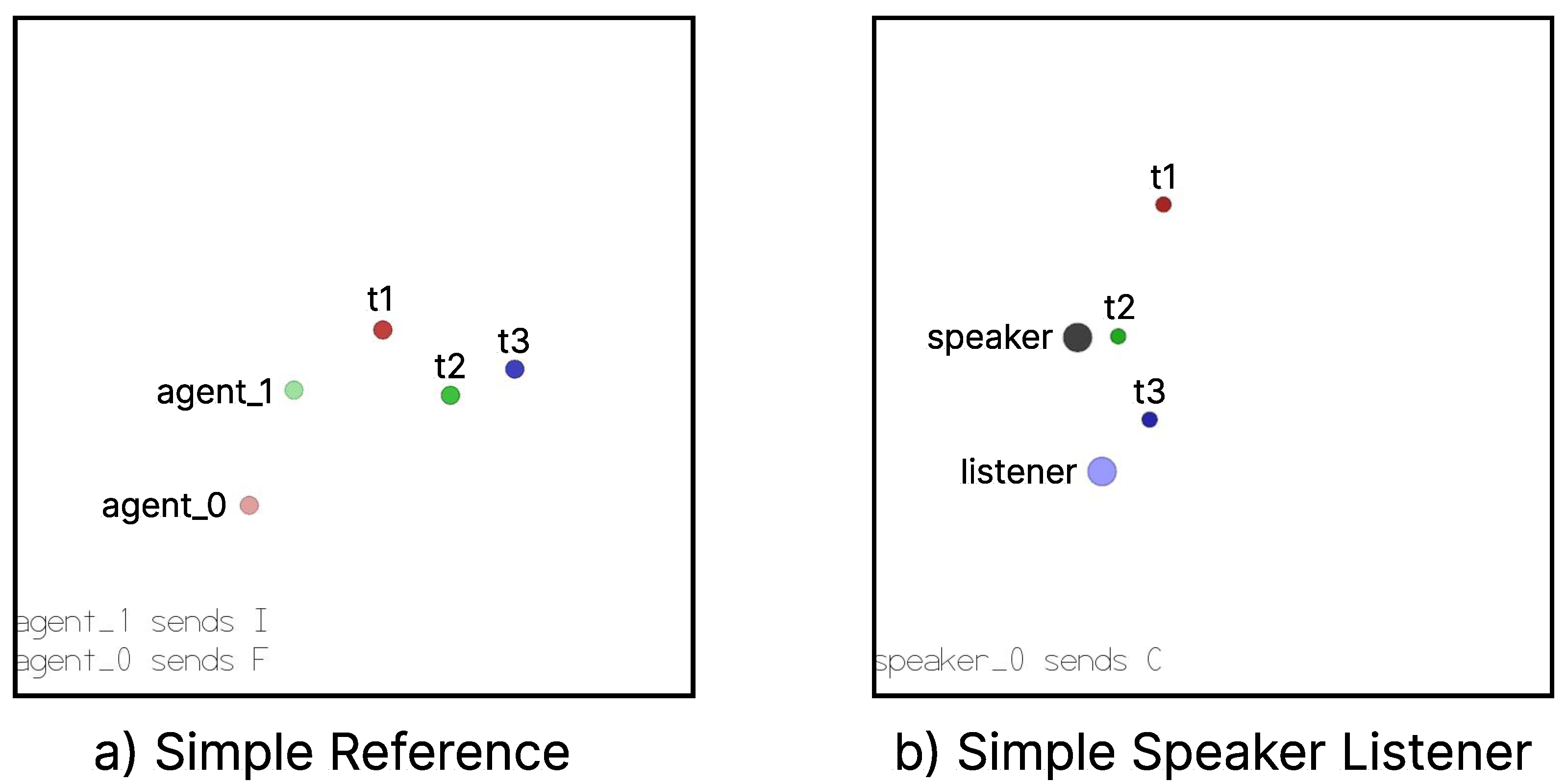
The simple_speaker_listener_v4 environment features two asymmetric agents and three color-coded targets, red (t1), green (t2), and blue (t3), as presented in Figure 1.

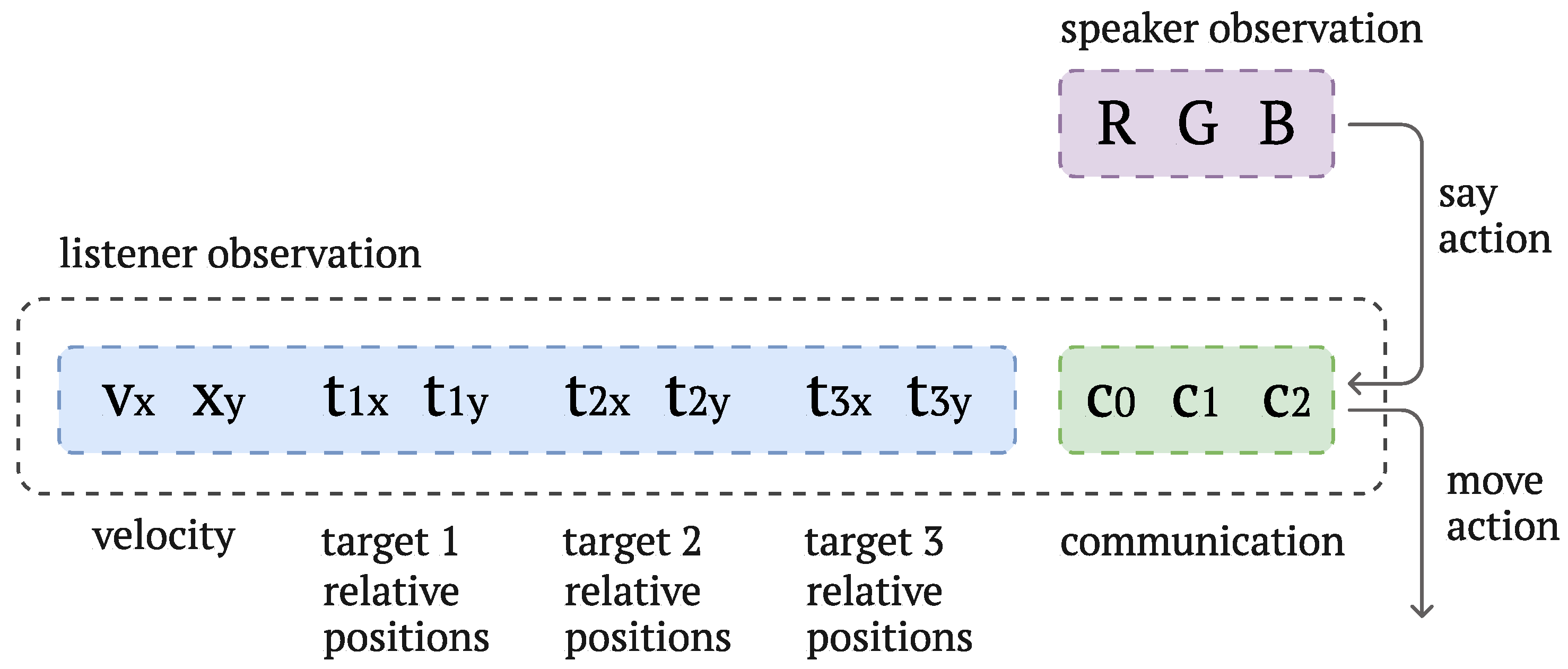
The speaker knows the target color for the current game episode and sends a discrete message to guide the listener. The listener perceives its movement direction, the relative distances to targets, and the speaker’s messages and can step horizontally, vertically, or not move at all (see Figure 2).

The same applies to the simple_reference_v3 environment, except that each agent simultaneously assumes the roles of both the speaker and the listener. In this environment, each agent knows the direction in which the other agent should move, but lacks the knowledge of its own target.

In simple_reference_v3, both agents receive rewards. The closer the agent is to its target, the greater the reward it receives. In simple_speaker_listener_v4, the speaker’s reward equals the listener’s reward. An episode ends either when the listener reaches the target or when a step limit is reached.

As the number of active agents within the environment increases, the overall action space expands with the Cartesian product of the sets of individual agent actions. Combined with the inherent stochasticity of agent policies, this increased complexity compounds reproducibility challenges related to the unstable convergence in reinforcement learning algorithms and heightened sensitivity to implementation details. To examine the role of communication decoupled from reciprocal navigation in a controlled experimental setting conducive to reliable evaluation, our study focused on the simple_speaker_listener_v4 environment.

4.2. Format Invariance

In agent-to-agent systems, the most prevalent forms of information include continuous signals, interval-based measurements, and categorical levels. When humans are incorporated into interactions with such systems, the range of information modalities expands further to include inputs such as audio commands and visual data (e.g., images, point clouds, and related representations).

Similarly, simulation environments such as simple_speaker_listener_v4 often comprise heterogeneous agents that differ in the nature of their observations.

To establish a foundation for scaling our game-based example to industry-specific applications, we employed the publicly available GPT-2 under the MIT license to vectorize input representations, irrespective of their original modality.

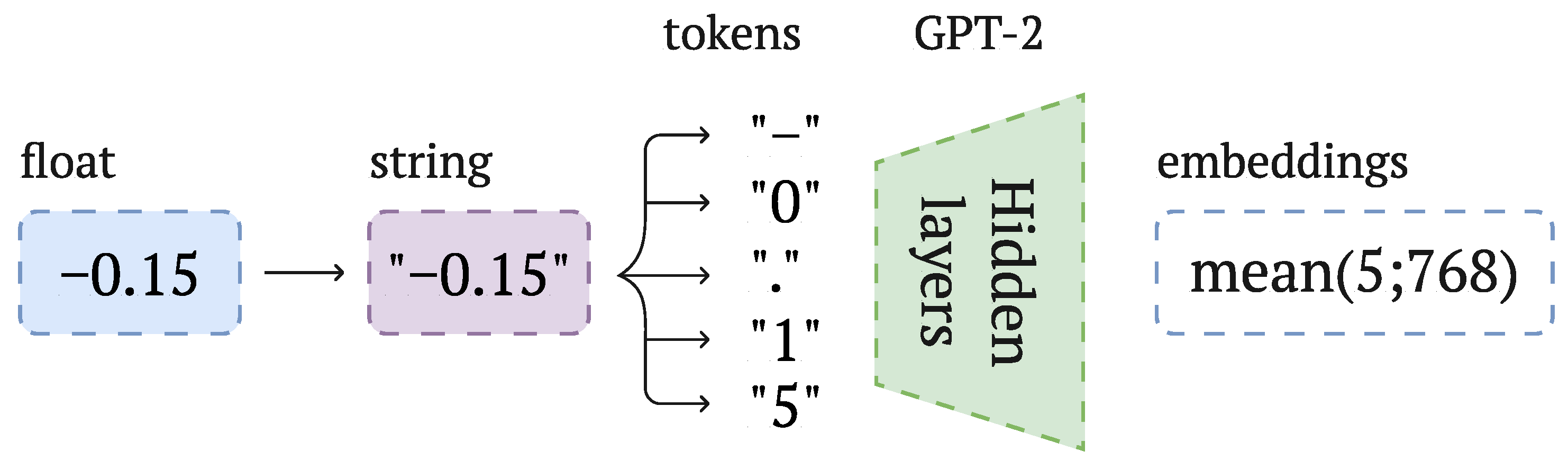
The listener agent is characterized by an observation space of dimensions $(1,11)$. Each element is represented as a floating-point number. To process these observations, each float was first converted into a string, as illustrated in Figure 3, and subsequently tokenized.

The resulting tokens, including numeric digits, signs, and decimal points, were passed to GPT-2 to extract vector representations of shape $(11,n,768)$, where n denotes the number of tokens generated from the string. These vectors were then averaged over n to obtain the shape of $(11,768)$.

The target label could also be represented in the form of an image. In this case, the preprocessing would remain largely unchanged, although handling this representation would require a more expressive, next-generation multimodal language model, such as GPT-4 mini.

4.3. Autoencoder

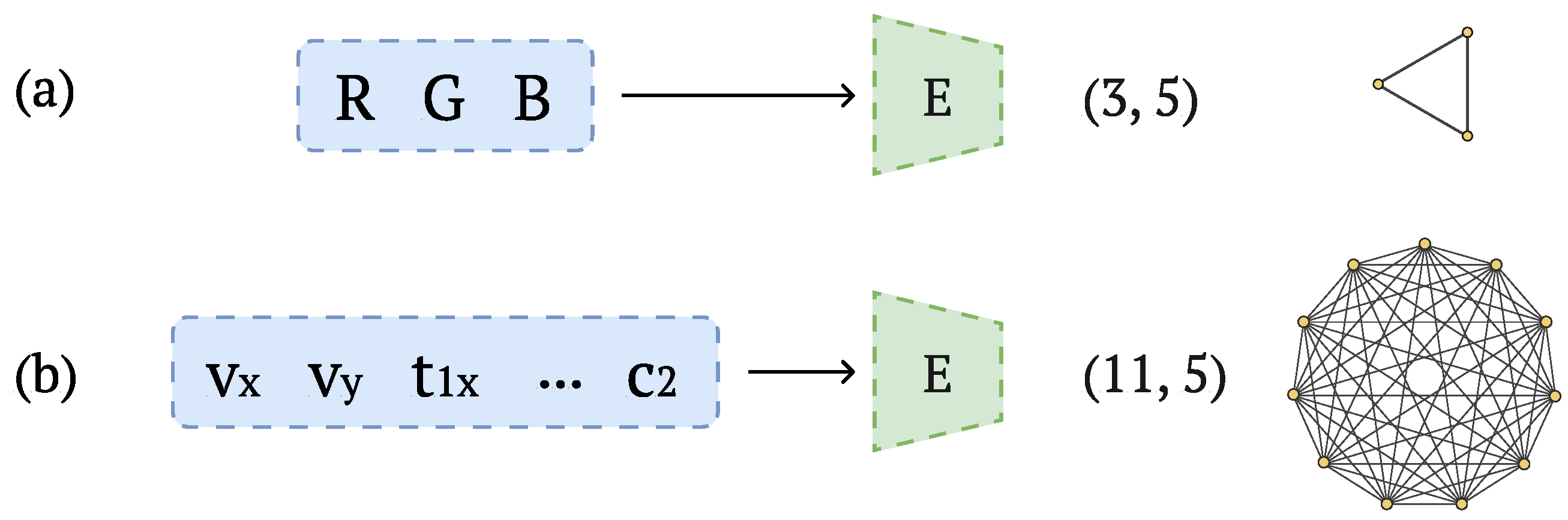
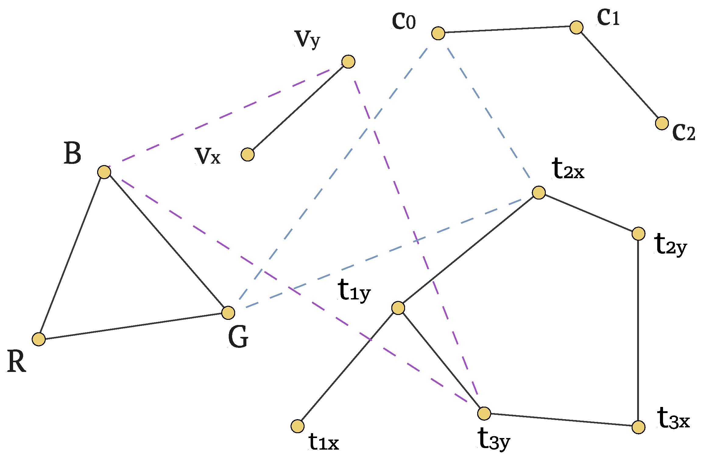
Spatial representation. To partition the agents’ observations into components that can be recombined to provide new topology and semantic information, we map them into a graph modality. Thus, each element of size $(1,768)$ from the observation vector $(n,768)$, where n varies according to the agent’s observation size, is fed into the input of a graph autoencoder and mapped to a triplet $(x,y,z)$ of size $(1,3)$, yielding $(n,3)$. The first two components, x and y, specify the node’s position, while z serves as the node’s feature (see Figure 4).

Creating a set of n nodes and connecting them into a complete graph yields a graph-based knowledge representation of the original observation vector. A set of nodes is also referred to as a cloud of points in surface reconstruction problems; this point cloud is combined into a graph in a way that directly impacts the fidelity of the reconstruction, as will be discussed below (see Section 5).

Latent Space Regularization. The latent space of a conventional autoencoder has no well-defined structure. In representation learning; however, regularizing the latent space is a crucial step for ensuring meaningful and consistent output.

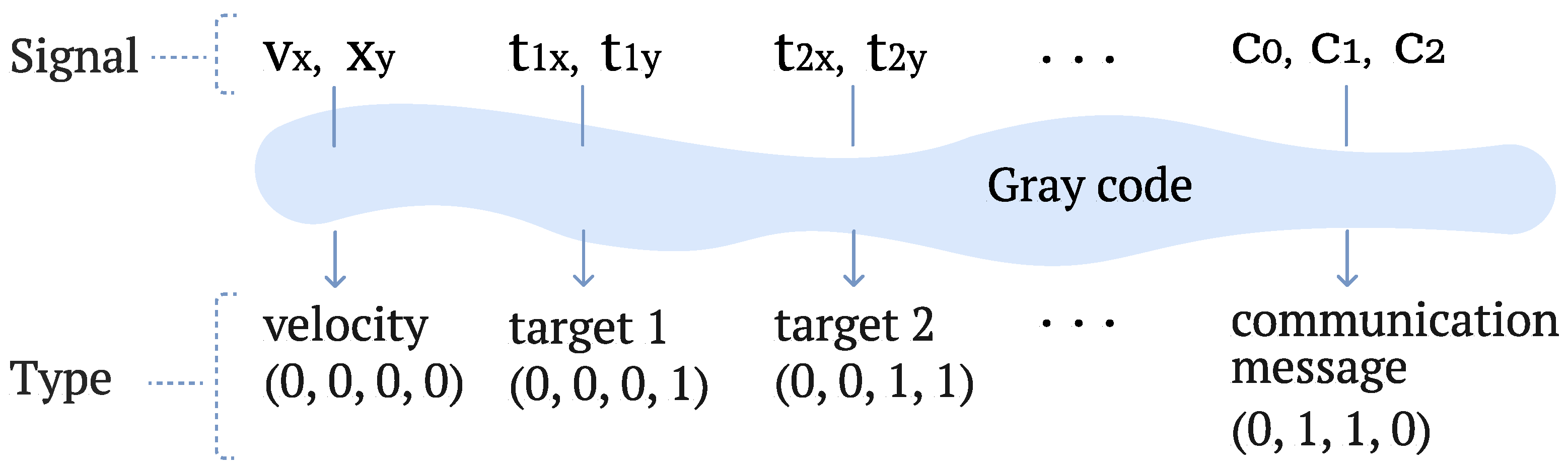
One approach to regularizing the structure of the latent space is to incorporate label information into the input data, as described for the CVAE in Section 3.1. Gray encoding is a binary numeral system in which consecutive values differ by only one bit, unlike standard binary encoding in which multiple bits can change at once.

This property ensures that semantically related information channels, for example, the projections of a velocity vector onto the x- and y-axes (see Figure 5), are positioned in close proximity within the latent space of the autoencoder network, which is time- and order-invariant, a common prerequisite among real-time applications.

Based on the number of unique information channels in our environment, we determined that four bits are sufficient. Consequently, after concatenating the gray encoding with a vector of size $(1,768)$, the resulting representation has dimensions $(1,772)$. It is also important to note that the encoding facilitated functional interpretability at the level of a machine learning engineer, particularly during the reverse deployment and analysis of training logs.

Another approach to imposing regularization on the latent representation encoded by a graph is to augment the autoencoder’s loss function with an additional penalty term. In our formulation, this regularization term corresponded to the sum of the absolute values of the graph’s edge lengths.

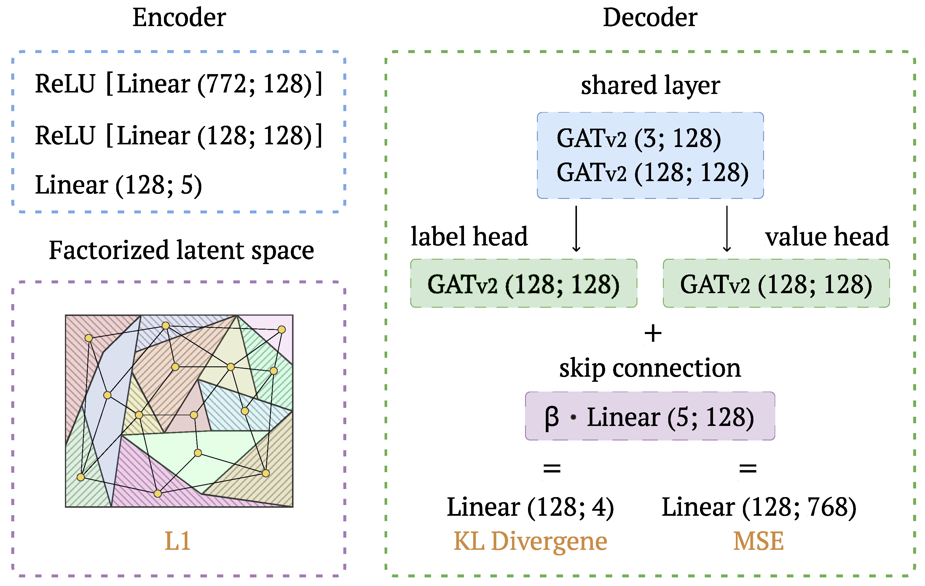
Training. The proposed autoencoder employed a three-layer MLP with ReLU activations to map input observations to a k-dimensional latent representation, where the first two dimensions served as spatial coordinates and the remaining $k-2$ dimensions constituted node features. Graph construction applied parameterizable criteria to the set of nodes, yielding connectivity patterns that encode spatial and semantic relationships. Two parallel GATv2 branches with residual connections processed the resulting knowledge graphs for reconstruction, terminating in specialized heads for categorical and continuous variable prediction, enabling the model to capture both the discrete and continuous components of an input $(1,772)$ observation vector (see Figure 6).

The loss function used in the training process extended the VAE and CVAE loss function described in Equations (2) and (3) in Section 3.1 so that the reconstruction loss is represented here as the sum of the first two components:

$${\mathcal{L}}_{total}=w_1\left(t\right){\mathcal{L}}_{KL}+w_2\left(t\right){\mathcal{L}}_{MSE}+\lambda {\mathcal{L}}_{L_1}$$

(10)

where ${\mathcal{L}}_{KL}$ is the Kullback–Leibler divergence between the predicted distribution and the softmax normalized gray encoded ground truth labels, ${\mathcal{L}}_{MSE}$ denotes the Mean Squared Error between the predicted and actual feature values, and ${\mathcal{L}}_{L_1}$ corresponds to the sum of absolute values applied to the edge distances. The time-dependent weighting coefficients $w_1\left(t\right)$ and $w_2\left(t\right)$ are inversely related, with $w_1\left(t\right)+w_2\left(t\right)=1.0$. The hyperparameter $\lambda$ controls the relative contribution of the edge regularization term to the overall loss.

4.4. Knowledge Graph Construction

The fidelity of reconstructing the original observation vectors depends on the edge selection mechanism. Conventional k-NN approaches employ fixed global connectivity parameters, which fail to adapt to local density variations, while geometric methods, such as Delaunay or Gabriel graphs, impose rigid spatial constraints that may fragment sparse regions, see Section 3.2, Equation (4). To overcome these limitations, we introduce a density-adaptive neighborhood selection strategy augmented with geometric pruning, thereby ensuring global connectivity, local density awareness, and geometric consistency within the constructed graphs.

For a set of vertices $V=\{v_1,\dots ,v_n\}\subset {\mathbb{R}}^d$ with base neighborhood size k, the local density at point $v_i$ is estimated as

$$d_i={\displaystyle \frac{1}{\frac{1}{k}{\sum }_{j=1}^k\parallel v_i-u_j\parallel +\epsilon }}$$

(11)

where $u_1,\dots ,u_k$ represent the k nearest neighbors of $v_i$ (excluding $v_i$ itself), and $\epsilon >0$ prevents numerical instability from division by zero.

The global median density $\tilde{d}=\mathrm{median}(d_1,\dots ,d_n)$ serves as a normalization reference. The adaptive neighborhood size for point $v_i$ is computed as

$$k_i^{\mathrm{adapt}}=⌊k·{\left({\displaystyle \frac{d_i}{\tilde{d}}}\right)}^{\alpha }⌋,k_i^{\mathrm{adapt}}\in [k_{min},k_{max}]$$

(12)

The parameter $\alpha >0$ controls the density sensitivity, while bounds $k_{min}$ and $k_{max}$ prevent node isolation and excessive connectivity, respectively.

To balance geometric locality with connectivity preservation, a $\beta$-relaxed Gabriel criterion is applied (see Equation (4), Section 3.2). An edge $(v_i,v_j)$ is retained if

$$\parallel v_k-m_{ij}\parallel \ge \beta ·{\displaystyle \frac{\parallel v_i-v_j\parallel }{2}}\forall v_k\in \mathcal{P}\setminus \{v_i,v_j\}$$

(13)

where $m_{ij}={\displaystyle \frac{v_i+v_j}{2}}$ denotes the edge midpoint, and $\beta \in (0,1]$ controls relaxation intensity. The classical Gabriel test corresponds to $\beta =1$, while $\beta <1$ permits the retention of additional edges.

The complete procedure is formalized in Algorithm 1.

Algorithm 1 Density-Adaptive k-NN Graph with Gabriel Pruning

Require:  Set of vertices $V=\{v_1,v_2,\dots ,v_n\}\subset {\mathbb{R}}^d$ Require:  Nearest neighbors $k\in \mathbb{N}$, default = 6 Require:  Density scaling factor $\alpha \in {\mathbb{R}}^{+}$, default = 1.5 Require:  Gabriel threshold $\beta \in (0,1]$, default = 1.0 Ensure:  Edge set $E\subseteq V\times V$   Construct KD-tree $\mathcal{T}$ from V   for $i=1$ to n do       $\{q_1,\dots ,q_k\}\leftarrow k-\mathrm{NN}(v_i,\mathcal{T})\setminus \left\{v_i\right\}$                                 ▹k-Nearest Neighbors       $d_i\leftarrow {\displaystyle \frac{1}{\frac{1}{k}{\sum }_{j=1}^k\parallel v_i-q_j\parallel +ϵ}}$                                                            ▹ Local density   end for   $\tilde{d}\leftarrow \mathrm{median}\left(\{d_1,\dots ,d_n\}\right)$                                                           ▹ Median density   Initialize $E\leftarrow \varnothing$   for $i=1$ to n do       $k_i^{\mathrm{adapt}}\leftarrow ⌊k·{\left({\displaystyle \frac{d_i}{\tilde{d}}}\right)}^{\alpha }⌋$                                                                      ▹ Adaptive k       $k_i^{\mathrm{adapt}}\leftarrow max(3,min(k_i^{\mathrm{adapt}},2k))$                                                     ▹ Bound k       ${\mathcal{N}}_i\leftarrow k_i^{\mathrm{adapt}}-\mathrm{NN}(v_i,\mathcal{T})\setminus \left\{v_i\right\}$       for each $v_j\in {\mathcal{N}}_i$ do           if $\mathrm{IsGabrielEdge}(v_i,v_j,V,\beta )$ then              $E\leftarrow E\cup \left\{(v_i,v_j)\right\}$           end if       end for   end forreturn E

The initial density computation utilizes KD-tree structures for efficient nearest neighbor queries. Following the median density calculation, adaptive neighborhood sizes are determined and clamped to specified bounds. The $\beta$-relaxed Gabriel criterion is then applied to candidate edges from each point’s adaptive neighborhood.

This hybrid approach provides tunable control over both the density adaptation through parameter $\alpha$ and the geometric pruning through parameter $\beta$, resulting in a unified framework for proximity graph construction that addresses the density–geometry trade-off inherent in existing methods.

4.5. Hypergraph Aggregation

The centers of the knowledge graphs produced with Algorithm 1 are translated within the game environment relative to the positions of their corresponding agents, after which the resulting m components are integrated into a hypergraph.

Let $m\ge 2$ and let $V_1,\dots ,V_m$ be a pairwise-disjoint finite set of vertices $V_i\subset {\mathbb{R}}^2$. The undirected symmetric k-NN graph on $V_i$ is $G_k\left(V_i\right)=(V_i,E_i)$, where $\{u,v\}\in E_i$ if u is among the k-NN of v in $V_i$ or vice versa. A hypergraph $H=(V,\mathcal{E})$ has a 2-section ${\left[H\right]}_2$ with $\{u,v\}\in {\left[H\right]}_2$ if some $e\in \mathcal{E}$ contains both u and v. A bridging hyperedge $e\subseteq V={\bigcup }_{i=1}^m{V}_i$ intersects vertices from at least two distinct $V_i$. See all definitions in Appendix A.1.

We aim to connect the m disjoint k-NN graphs by adding minimal bridging hyperedges while satisfying the set properties (see Appendix A.2). We assume each $G_k\left(V_i\right)$ is in its general position and the feasibility graph F on $\{1,\dots ,m\}$ is connected. Here, indices $i,j\in \{1,\dots ,m\}$ label the base components or agent knowledge graphs.

Let $t^{\star }$ be the minimum number of bridging hyperedges needed. Under Assumptions A1–A3 (see Appendix A.3), we then derive the tight bounds as follows:

Theorem 1

(Bridging bounds).

$$⌈\frac{m-1}{r-1}⌉\le t^{\star }\le m-1$$

Proof of Theorem 1.

Let C be the number of connected components in the 2-section induced by the m blocks before adding any bridging hyperedges; initially, $C=m$.

Lower bound. Suppose a bridging hyperedge e intersects with q distinct components. Then, e can reduce C by at most $q-1$. Since $\left|e\right|\le r$, necessarily $q\le r$, so each hyperedge reduces C by at most $r-1$. To achieve $C=1$ from $C=m$, we need a total decrease of $m-1$, and hence, at least $\lceil (m-1)/(r-1)\rceil$ hyperedges. Upper bound. Since the feasibility graph F is connected, let T be any spanning tree of F. For each edge $\{i,j\}\in T$, pick feasible representatives $u\in V_i$ and $v\in V_j$ (with $\parallel u-v\parallel \le 2\rho$ if locality is enforced) and add the bridging hyperedge $\{u,v\}$. Each addition reduces C by one, so after $m-1$ additions, the 2-section is connected. Thus, $t^{\star }\le m-1$. Tightness. (i) If geometry allows a single location to meet r components, then $\lceil (m-1)/(r-1)\rceil$ star-like hyperedges can be created, each containing an anchor vertex and up to $r-1$ vertices from previously unconnected components. This determines the lower bound. (ii) Conversely, let us suppose the m components are arranged in a chain under locality such that any radius-$\rho$ disk intersects the vertices from at most two components while adjacent components are feasible. Then, every bridging hyperedge can reduce C by at most 1, forcing $t^{\star }\ge m-1$, and the tree construction is optimal.  □

A geometry-aware refinement, accounting for effective arity under locality constraints, is provided in Appendix A.4.

Algorithm 2 returns a hypergraph that has at most $m-1$ bridging hyperedges and achieves exactly $⌈(m-1)/(r-1)⌉$ bridging hyperedges when geometry permits consistent $(r-1)$-way merges.

Algorithm 2 Bridging Hypergraph

Require:  Pairwise-disjoint finite set of vertices $V_1,\dots ,V_m\subset {\mathbb{R}}^2$ Require:  Nearest neighbors $k\ge 1$, default = 3 Require:  Arity cap $r\ge 2$, default = 4 Require:  Radius $\rho >0$, default = 1.5 Require:  Degree cap $L\in \mathbb{N}$, default = 3 Ensure:  Base k-NN graphs are connected   Initialize $V\leftarrow {\bigcup }_{i=1}^m{V}_i$;   $\mathcal{E}\leftarrow ⌀$.   for $i=1$ to m do                                           ▹ retain base k-NN graphs as size-2 hyperedges       build $G_k\left(V_i\right)=(V_i,E_i)$;    $\mathcal{E}\leftarrow \mathcal{E}\cup \{\{u,v\}:\{u,v\}\in E_i\}$.   end for   Build feasibility matrix $\mathsf{feasible}[i,j]\leftarrow$true if $\exists u\in V_i,v\in V_j$ with (no radius constraint) or $∥u-v∥\le 2\rho$.   Initialize a disjoint-set union (DSU) over components $\{1,\dots ,m\}$.   Choose an anchor component $a\in \{1,\dots ,m\}$ with maximum number of feasible neighbors.   $S\leftarrow \left\{a\right\}$;    maintain per-vertex load counters to enforce degree cap L.   while  $\left|S\right|<m$  do       $\mathsf{CAND}\leftarrow \{j\notin S:\mathsf{feasible}[a,j\left]\right\}$ filtered to respect load cap L.       Select $J\subseteq \mathsf{CAND}$ with $\left|J\right|\le r-1$ maximizing a tie-break score (e.g., nearest to a, balances loads, boosts global coverage).       if $J\ne ⌀$ then                                           ▹$(r-1)$-way merge when geometry allows           choose representatives $u_a\in V_a$ and $v_j\in V_j$ for $j\in J$ minimizing ${max}_{j\in J}∥u_a-v_j∥$;           add hyperedge $e\leftarrow \left\{u_a\right\}\cup \{v_j:j\in J\}$ to $\mathcal{E}$;    increment loads of involved vertices;           for $j\in J$ do              union DSU $(a,j)$;           end for           $S\leftarrow S\cup J$.       else                                           ▹ fallback ensures progress along a spanning tree of F           pick any $j\notin S$ with $\mathsf{feasible}[a,j]=\mathbf{true}$;           choose $(u,v)\in V_a\times V_j$ minimizing $∥u-v∥$; add hyperedge $\{u,v\}$ to $\mathcal{E}$; union DSU $(a,j)$;           $S\leftarrow S\cup \left\{j\right\}$.       end if       Optionally reset $a\leftarrow {arg\; min}_{i\in S}$ (estimated future cost) or the node in S with most feasible neighbors in $\overline{S}$.   end while   return $H=(V,\mathcal{E})$.

The algorithm maintains correctness by construction: the base graphs are preserved as size-2 hyperedges, connectivity follows from the union–find merging process, and constraints are enforced during candidate selection. The edge count bound results from each iteration, reducing the component count by at least one, which requires at most $m-1$ iterations, while optimal merges achieve the theoretical lower bound.

4.6. Experiment Design

We used the environment described in Section 4.1 with the step limit set at 25. When the step limit is reached, the game episode ends, even if the goal has not been achieved. The game may also end earlier than after 25 steps, making the actual number of game episodes variable given a fixed number of global training steps for the RL algorithm.

To standardize all input data and enrich the hidden representations, we leveraged the capabilities of the large-scale GPT-2 language model (MIT license). To extract the embeddings for multinomial input tokens, we applied mean pooling, as described in Section 4.2.

After collecting 10,000 observations from the environment, we constructed a dataset for training the GAE model, the operational principles of which are detailed in Section 4.3. Using randomly sampled batches of 128 instances, the GAE model was trained to project vectors of continuous values onto graph structures, with the edges produced according to Algorithm 1, as described in Section 4.4. The training objective, defined in Equation (10), consists of a weighted sum of reconstruction and regularization loss functions, with the corresponding weights linearly annealed over 30 epochs. Gradient clipping was applied with a maximum norm of 1.0. The Adam optimizer was employed with a learning rate of $2.5\times {10}^{-3}$, and a ReduceLROnPlateau scheduler was utilized with a reduction factor of 0.5 and a patience of 5 epochs.

During the training of the reinforcement learning agents, the weights of the GAE model were kept frozen. When the agents entered the bridging zone, their observation vectors were provided as inputs to the GAE. The resulting graphs were subsequently translated according to the agents’ positions in the environment. Following the constraints outlined in Theorem 1 from Section 4.5, Algorithm 2 was then employed to construct a shared knowledge hypergraph.

The graph-derived embeddings produced with the GAE were concatenated with the agent’s raw observation vectors to form an augmented state representation, which was then passed to the DQN online and target networks. Specifically, the GAT-based hypergraph handler consisted of three GATv2Conv layers with two attention heads in the first two layers and one head in the final layer, processing 3-dimensional node features through a hidden size of 64 to produce a 128-dimensional graph-level representation via global sum pooling. This graph embedding was then combined with a 14-dimensional raw observation vector using a fixed skip connection with the weight $\alpha =1.0$, while the raw observations were first projected to 128 dimensions through a learned linear transformation. The resulting 128-dimensional augmented state was processed through a multi-layer perceptron with ReLU activations and dropout regularization. The speaker q-network used a three-layer MLP with the layer decreasing from 128 down to the action dimension, while the listener q-network employed a deeper four-layer architecture decreasing from 256 down to the action dimension. Both networks used orthogonal weight initialization and a dropout rate of 0.1 between the hidden layers for improved training stability. The objective function optimized by these networks is defined in Equation (7) above, along with the complementary reinforcement learning formulation and the related training details.

Training protocol. To ensure that any observed performance difference stemmed solely from the inclusion of hypergraph features, both solutions were trained under identical conditions:

• Optimizer: Adam with a learning rate of $5\times {10}^{-4}$.
• Training steps: 10,000 environment interactions.
• Replay: Shared buffer capacity of 51,200 transitions; batch size of 128; learning starts after 1000 steps with one update every 5 steps.
• Targets: Soft target updates every 100 steps with rate $\tau =0.01$.
• Discount and rewards: $\gamma =0.99$; per-agent rewards are clipped to $[-\sqrt{2},\sqrt{2}]$ before computing TD targets.
• Exploration: $ϵ$-greedy linearly annealed from 1.0 to 0.05 over the first 10% of the training steps.
• Regularization: Dropout rate of 0.1; gradient is clipped with a maximum norm of 1.0; orthogonal weight is initialized with a gain of $\sqrt{2}$.
• Loss function: Smooth Huber loss for both agents.

Hyperparameter selection. Hyperparameters for both algorithms were selected using the Tree-Structured Parzen Estimator implemented in Optuna 4.5.0 (MIT license) [59].

Reproducibility. To ensure reproducibility, we conducted experiments across multiple random seeds and reported the mean and one standard deviation for all metrics. Deterministic behavior was enforced by setting random seeds for PettingZoo 1.24.3 (MIT license), Python 3.12 (PSF license), NumPy 2.2.5 (BSD-3 license), PyTorch 2.7.0 (BSD license), and PyTorch Geometric 2.6.1 (MIT license), with deterministic cuDNN operations possible where applicable.

Computational Environment. Intel Xeon 2.20 GHz, NVIDIA Tesla V100, 16 GB of RAM, Ubuntu 22.04.

5. Results and Discussion

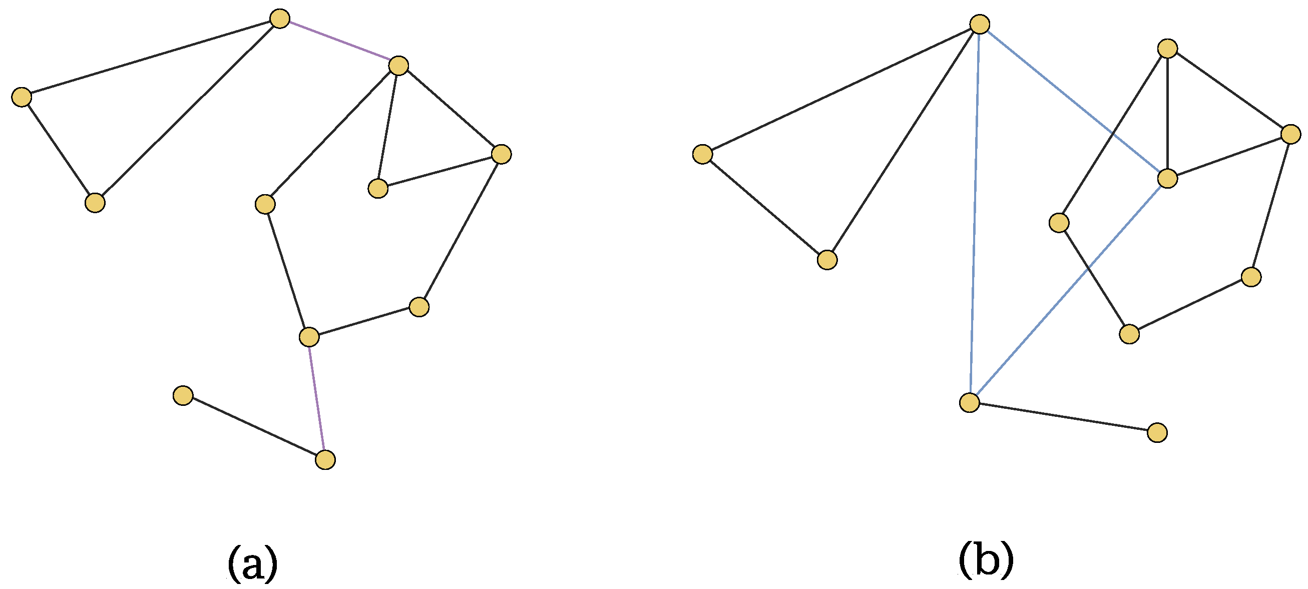
Figure 7 shows examples of the comparison algorithms in constructing a graph based on a given set of nodes.

As shown in Figure 7e, Algorithm 1 generates a noticeably sparser graph in high-density regions, while introducing additional edges to maintain global connectivity.

Table 1. Loss components across graph algorithms at the final epoch ($\mathrm{epoch}=30$), averaged over 100 random seeds.

Algorithm	${\mathcal{L}}_{\mathit{KL}}$	${\mathcal{L}}_{\mathit{MSE}}$	${\mathcal{L}}_{{\mathit{L}}_1}$	${\mathcal{L}}_{\mathbf{total}}$
k-NN + pruning	3.6 × ${10}^{-3}$ ± 2.8 × ${10}^{-3}$	3.8 × ${10}^{-2}$ ± 3.1 × ${10}^{-2}$	7.2 × ${10}^{-3}$ ± 1.0 × ${10}^{-3}$	4.9 × ${10}^{-2}$ ± 3.2 × ${10}^{-2}$
Gabriel	4.0 × ${10}^{-3}$ ± 3.1 × ${10}^{-3}$	4.9 × ${10}^{-2}$ ± 4.8 × ${10}^{-2}$	1.1 × ${10}^{-2}$ ± 1.4 × ${10}^{-3}$	6.4 × ${10}^{-2}$ ± 5.0 × ${10}^{-2}$
Complete	6.6 × ${10}^{-3}$ ± 3.7 × ${10}^{-3}$	4.7 × ${10}^{-2}$ ± 2.9 × ${10}^{-2}$	3.3 × ${10}^{-2}$ ± 5.8 × ${10}^{-3}$	8.6 × ${10}^{-2}$ ± 3.2 × ${10}^{-2}$
Delaunay	3.5 × ${10}^{-3}$ ± 2.1 × ${10}^{-3}$	4.2 × ${10}^{-2}$ ± 3.2 × ${10}^{-2}$	1.7 × ${10}^{-2}$ ± 2.4 × ${10}^{-3}$	6.2 × ${10}^{-2}$ ± 3.3 × ${10}^{-2}$
k-NN	3.7 × ${10}^{-3}$ ± 2.5 × ${10}^{-3}$	5.9 × ${10}^{-2}$ ± 5.4 × ${10}^{-2}$	1.7 × ${10}^{-2}$ ± 2.2 × ${10}^{-3}$	8.0 × ${10}^{-2}$ ± 5.4 × ${10}^{-2}$

Note: The table presents the mean ± one standard deviation. The best results among the compared algorithms are indicated in bold. The mean difference in the total loss between k-NN + pruning and its closest competitor, Delaunay, was $1.38\times {10}^{-2}$ with a 95% bootstrap confidence interval of $[4.6\times {10}^{-3},2.31\times {10}^{-2}]$.

presents the empirical distribution of component-wise errors.

The multi-component loss function $\mathcal{L}$ evaluates the observation label recovery using KL divergence, while continuous values are assessed via the MSE. An additional L1 regularization term penalizes the total weight of edges in the graph.

Figure 8 illustrates various instances for constructing a hypergraph using Algorithm 2, corresponding to various arity constraints, with the number of hyperedges that lie within the bounds established by Theorem 1.

Varying the hyperedge arity constraint captures the levels of relational complexity in a system, from pairwise relationships to higher-order interactions.

Figure 9 presents the resulting knowledge graphs generated with Algorithm 2 for both the speaker and the listener agents within the simple_speaker_listener_v4 environment.

When the message passes in the GAT layers, the information propagates across the nodes via attention-weighted aggregation, where the learned attention coefficients modulate the strength of communication between the neighboring nodes.

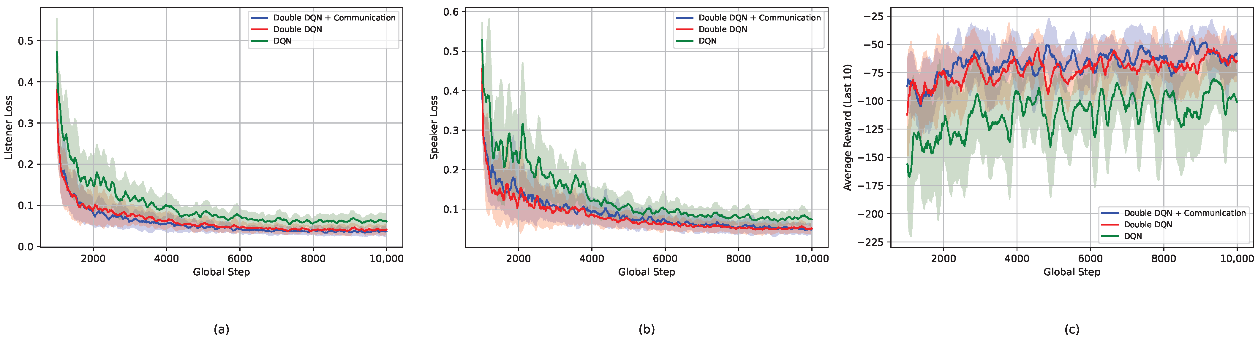
We assessed both the agent-specific metrics (speaker and listener policy losses) and the system-level performance (agent and episode rewards). Figure 10 presents the learning curves recorded.

The speaker error decreases at a slower initial rate, but ultimately converges to lower values. Moreover, the listener error exhibits a faster decay and then also attains smaller values. The rolling average of episode rewards highlights the systematic advantage of incorporating graph communication over the DQN baseline.

Table 2. Return comparison.

Metric	Baseline + Comm.	DDQN	DQN
Episode Reward
Overall avg. reward	−67.06 ± 58.18	−76.06 ± 63.42	−173.12 ± 97.92
Best step over all seeds	−41.63 ± 39.96	−53.59 ± 49.69	−106.47 ± 52.17
Agent Reward
Overall avg. reward	−5.54 ± 5.70	−6.51 ± 6.33	−16.46 ± 9.55
Best step over all seeds	−2.48 ± 2.35	−4.18 ± 4.59	−10.93 ± 6.67

Note: The table presents the values of the mean ± one standard deviation. The best results among the compared algorithms are in bold. The mean difference in the overall average episodic reward between Baseline + Comm. and its closest competitor (DDQN) was 7.24, with a 95% bootstrap confidence interval of [1.03, 13.91]. For the overall average agent reward, the mean difference was 0.81, with a 95% bootstrap confidence interval of [0.18, 1.45].

provides a comprehensive comparison of the return metrics across both configurations.

All performance values are reported as the mean and standard deviation over the 10 random seeds in each training step, ensuring reliable convergence estimates. The interval values of the metrics are given in Appendix B.

Our primary configuration demonstrated meaningful improvements over the baseline, achieving $\approx 10.0\%$ higher episode rewards ($-67.06\pm 58.18$ vs. $-76.06\pm 63.42$), and up to 40.0% better individual agent rewards ($-2.48\pm 2.35$ vs. $-4.18\pm 4.59$), while maintaining comparable policy loss values. These results suggest that the hypergraph communication mechanism helps capture the semantic complexities of the paired observation space.

The results of the ablation analysis conducted across three random seeds suggest that different data preprocessing variants exert only an incremental impact on the performance of the proposed framework (see Appendix C). The addition of Gray Code, while computationally inexpensive, appears to account for most of the observed performance differences by conditioning the latent space of the autoencoder model, whereas input standardization using GPT embeddings seems to have contributed less in this setting. As increased computational complexity can introduce additional operational costs during deployment, the decision to incorporate GPT embeddings therefore needs to be evaluated on a case-by-case basis, which may prove valuable in scenarios involving more diverse or multimodal observation structures.

6. Conclusions and Future Work

This work introduces a neuro-symbolic framework that addresses coordination challenges in multi-agent systems through structured knowledge representations. Two algorithms form the core of the approach: One is a density-adaptive k-NN graph construction method that adjusts neighborhood sizes to local point density while maintaining geometric consistency through Gabriel pruning. The other is a hypergraph aggregation algorithm with tight bounds on the minimum number of bridging hyperedges required under arity and locality constraints.

Empirical validation on PettingZoo’s communication-oriented environment demonstrates meaningful performance gains: approximately 10% improvement in episode rewards ($-67.06\pm 58.18$ vs. $-76.06\pm 63.42$) and up to 40% improvement in individual agent rewards ($-2.48\pm 2.35$ vs. $-4.18\pm 4.59$) compared to DQN baselines, while maintaining comparable policy loss values. The framework successfully handles heterogeneous observations through language model embeddings for format-invariant preprocessing, while gray encoding regularizes the latent space to ensure semantic coherence across agent knowledge graphs.

The combination of density-adaptive k-NN construction and hypergraph-level arity constraints provides architectural benefits beyond the reported performance improvements. Our graph construction method achieves a lower total reconstruction loss (4.9 × ${10}^{-2}$ ± 3.2 × ${10}^{-2}$) than that of certain alternatives, including Gabriel graphs (6.4 × ${10}^{-2}$ ± 5.0 × ${10}^{-2}$), Delaunay Triangulation (6.2 × ${10}^{-2}$ ± 3.3 × ${10}^{-2}$), and conventional k-NN (8.0 × ${10}^{-2}$ ± 5.4 × ${10}^{-2}$). Specifically, localized connectivity and bounded hyperedge cardinality mitigate over-smoothing and over-squashing effects—well-documented challenges in deep graph architectures that degrade learning. By maintaining stable message-passing dynamics and improved gradient flow across subgraph boundaries, the approach establishes a foundation for scalable deployment in IoA ecosystems, where interpretability is mandated by regulatory frameworks and communication efficiency directly impacts operational costs [60,61]. The explicit graph structures enable the post hoc auditing of agent interactions and facilitate the integration of domain-specific constraints—capabilities increasingly required for industrial IoA deployments in safety-critical sectors such as smart manufacturing, autonomous logistics, and distributed energy management.

While the proposed algorithms impose no explicit restrictions on graph expansion, the GATv2 performance degrades as the number of hypergraph components increases. This limitation remains manageable for the two-level hierarchical system presented here and can be further alleviated. Thus, future work should investigate sampling-based architectures such as GraphSAGE [62] or minibatch training strategies that maintain scalability without sacrificing representation quality for larger-scale deployments. Beyond the ablation analysis employed, comprehensive evaluation of the framework’s robustness across diverse multi-agent scenarios remains an important direction for future work. Additionally, group-theoretic structures, particularly Cayley graphs, offer promising mathematical foundations for high-level agent planning. Such representations could encode action sequences and behavioral patterns as group elements, potentially enabling more structured exploration of the policy space and providing algebraic constraints that guide coordination in complex multi-agent tasks.

The framework’s modular design positions it for integration with emerging neuro-symbolic reasoning methods, establishing a path toward more transparent and governable distributed intelligent systems.