Abstract
Dynamic stall is a phenomenon on the retreating blade of a helicopter which can lead to excessive control loads. In order to understand dynamic stall and fill the gap between the investigations on pitching wings and full helicopter rotor blades, a numerical investigation of a single rotating and pitching blade is carried out. The flow phenomena thereupon including the -shaped dynamic stall vortex, the interaction of the leading edge vortex with the tip vortex, and a newly noticed vortex structure originating inboard are examined; they show similarities to pitching wings, while also possessing their unique features of a rotating system. The leading edge/tip vortex interaction dominates the post-stall stage. A newly noticed swell structure is observed to have a great impact on the load in the post-stall stage. With such a high Reynolds number, the Coriolis force exerted on the leading edge vortex is negligible compared to the pressure force. The force history/vortex structure of the slice = 0.898 is compared with a 2D pitching airfoil with the same harmonic pitch motion, and the current simulation shows the important role played by the swell structure in the recovery stage.
1. Introduction
Dynamic stall on the retreating blade of a helicopter is a factor that inhibits the progress of fast forward flight or manoeuvre flight; the subsequent aero-elastic response of the blade serves as a main source of vibrations and high structure loads. Since the discovery of dynamic stall, it has been a heated topic in the helicopter community. Understanding the phenomenon to implement effective flow control to ease the structural loads is the main purpose of the research.
Numerous experimental investigations [1,2,3,4,5] on oscillating airfoils; especially, the NACA 0012 airfoil was carried out in order to understand the mechanism of dynamic stall, as well as how the airfoil type, pitching amplitude, pitching rate, reduced frequency and the compressible effect impact aerodynamic coefficients. Ref. [6] used smoke as a flow indicator, showing the vortex shedding process over both small and large amplitude oscillations. Ref. [7] summarised early progress made in understanding dynamic stall, including the contribution of the dynamic stall vortex shedding to the surge of the normal force, the chord-wise force and the negative pitch moment; the role that reduced frequency or the pitching rate plays in the process; and the onset of vortex shedding as a result of the reverse flow upstream propagation from the trailing edge.
With the development of computational fluid dynamics in the late 1990s, many numerical simulations were carried out and compared with experimental data [8,9,10,11]. It was soon realized that 2D laminar simulations generally underestimate the unsteady load, while 2D simulations with turbulence models usually over-estimate the load. Experiments and numerical simulations on full rotor blades suggest a more complex flow structure, motivating research on vortex propagation [12] and the three-dimensional (3D) effect [13,14,15,16] on dynamic stall. Refs. [14,16] have done various experiments as well as numerical simulations on two types of pitching finite wings (OA209 blade and DSA-9A wing with parabolic tip) at DLR (German Aerospace Center). In their research, they showed that 2D dynamic stall is similar to the slice on a 3D pitching wing at the position where the dynamic stall is triggered but differs significantly in other areas. Comparing with experiment results, they found that Menter’s Shear Stress Transport turbulent model (Menter SST model) provided a closer force prediction than the Spalart–Allmaras model. For both types of wings, an -type dynamic stall vortex was observed on the wing and was responsible for the stall force hysteresis. Ref. [15] carried out high fidelity large eddy simulation (LES) on a pitching NACA 0012 finite wing and elucidated the onset of dynamic stall on a 3D wing. The same as for the 2D case, dynamic stall is triggered by the bursting of the laminar separation bubble. Additionally, they also described the behavior of the subsequent shaped vortex and an arched vortex.
Many researchers also presented experiments and numerical simulations to illustrate the rotating effect of the flow structure on a moving blade. Ref. [17] investigated the radial jet-like layer experimentally, showed the breaking away of discrete structures in the radial flow, and found that the dynamic stall event is strongly dependent on radial locations. Ref. [18] carried out numerical simulations using implicit large eddy simulation on quasi-3D airfoil sections for dynamic stall cases considering the yawing, surging and Coriolis effect. They concluded that rotational acceleration and yawing effect do not influence the attached boundary thickness, but the dynamic stall vortex (DSV) is shed sooner due to a weaker trailing edge vortex (TEV) in the case of the yawing effect. Ref. [19] did a numerical investigation on a rotating wing with a fixed aspect ratio at a low Reynolds number. They explained how the Rossby number (the ratio of inertial force to Coriolis force) affected the vortex structure on the wing, and discussed how the balance of the centrifugal force and Coriolis force stabilized the leading-edge vortex. Ref. [20] performed experiments and numerical simulations on a rotor with cyclic pitch control. In the experiment, they showed that both the FLOWer solver and DLR-TAU solver with the Menter SST model yield results similar to the experiments. Furthermore, they also reported failure of prediction of dynamic stall by both solvers when using the Spalart–Allmaras model (SA model). In contrast to the DLR-TAU solver, the URANS FLOWer solver showed an -shaped dynamic stall vortex on the blade. Ref. [21] carried out experiments and numerical simulations on the 7A rotor with trimmed cyclic control. He showed the chord-wise flow separation point in a rotor map, which indicates three different types of separation areas, namely the trailing-edge separation, leading-edge separation and the shock-induced separation. Moreover, in his research, the tip vortex of the previous blade was shown to trigger dynamic stall on the posterior blade inboard.
The stall onset mechanism on 2D airfoil and 3D pitching wing is understood through thorough experiments and high fidelity numerical simulations. However, the stall event on a helicopter’s retreating blade is far from a complete picture. Since modern rotor blades are possibly designed along the span with different airfoil types, linear twist, tapered or parabolic tip; these complex parameters of the real rotor blade, as well as the yet unclear role played by the rotation, blade/vortex interaction(BVI) make the understanding of DS mechanism on the helicopter environment more difficult. Without understanding this, the development of the lower-order aerodynamic model would be of little progress. In order to fill the gap from a pitching wing to 2- or 4-bladed real rotor, we thus propose an investigation of dynamic stall on a single rectangular blade with a curved tip under cyclic pitch control given by comprehensive-analysis (CA), hence eliminating the effect of BVI, twist and tip shape effects. The results can be compared to a pitching airfoil to illustrate the rotational effect.
This paper is organized as follows: The numerical setups of both comprehensive-analysis and computational fluid dynamics are described in Section 2. The numerical results and discussions of the phenomena associated with stall on the retreating blade are presented in Section 3. Moreover, the conclusions and outlook for future work is in the final section. In order not to destroy the continuity of the text, the grid convergence study, as well as the validation of grid strategy and turbulence model on the hovering case of Caradonna–Tung blades are placed in Appendix A and Appendix B, respectively.
2. Numerical Method
Flow Configuration and Numerical Setup
Currently, the chair of helicopter technology of the Department of Aerospace and Geodesy, TUM is preparing an experiment on measuring flow field and pressure on a single rotating blade. The simulation serves as a preliminary investigation of the phenomenon. According to the principle of simplicity, the blade is chosen to be, similar to the Caradonna–Tung blade, a rectangular blade with the NACA 0012 profile without a twist along the span. In order to mount pressure sensors thereon, the chord is selected to be c = 0.15 m in the first place; and in order to fit into the wind tunnel at Department of Mechanical Engineering, TUM, the span is selected as R = 0.8 m. The blade model used for the simulation is built by extruding the airfoil profile from to ; tips are rounded by revolving the half of the airfoil profile about its chord.
The advance ratio is set to be and rotation speed of the rotor be 275 rad/s or 2626.056 rpm; the rotor has 0 shaft angle and no flap, and the control is with a trim condition: thrust N , and , given by CAMRAD II [22] as: collective pitch , cyclic pitch and . We have to state that the pitch control is based on the lower-order aerodynamic model in CAMRAD II, which doesn’t necessarily guarantee the desired operation condition in real case. This work is a preliminary investigation of the dynamic stall phenomena on the retreating blade prior to the experiment, hence the deviation is tolerant and the control yielded by CAMRAD II is accepted as the setting for the rotor. Mathematically speaking, the pitch follows:
The flow condition for the rotor is summarised in Table 1. The computation is performed with the URANS code DLR-TAU [23]. Previous research has extensively validated that this code is capable of predicting dynamic stall on pitching wings [14,24], as well as for rotors [20]. For our case, a chimera technique is utilized, and the computation domain is split into three blocks: innermost blade block (Figure 1a) that resolves boundary layer on the blade and it does pure pitching; the outmost far-field block (Figure 1c) with multi-resolution voxel grid refined with an inclined cylindrical ring volume that tracks the tip vortex; and the rotating block in-between (Figure 1b) with relatively uniform spaced cells, through which the tip vortex is convected to the far-field, and it does pure rotation. The flow information of each block is exchanged in the chimera region.

Table 1.
Flow condition.
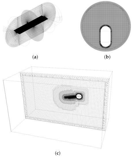
Figure 1.
Configuration of the mesh: (a) blade block; (b) voxel rotating block; (c) voxel far-field block.
The surface mesh on the blade is constructed to have a closer spatial resolution with simulations done by [21,24,25]. The spatial resolution of the blade block for the current simulation is summarized in Table 2. The blade block has a dimension of 3.2 c (3.2 times chord length) in radius and 6.76 c in length; it is constructed by extruding firstly the surface mesh normally 60 steps, and an O-type block is then assembled outside the boundary region; the overset mesh is constructed by extruding the outer surface mesh of the blade block algebraically 5 steps outward. The surface mesh has 11 million cells. The rotating block is a spherical volume with 5 c as radius, centering at the blade’s rotation center; the voxel grid is generated between the outer surface of the previous overset mesh and the spherical surface domain. The average space in this block is around 5.9% c; the maximum space appears in the zipping region near the spherical surface 15% c. The chimera mesh is then constructed the same way by extruding equal spaced 6.67% c for five steps. The rotating block has 15.2 million cells. The farfield block extends upstream 15 R, downstream 35 R, upward 11.22 R, and downward 19.24 R, both sides horizontally 15 R. The voxel grid is utilized to generate finely spaced grid near the rotating blade and step by step coarsened till the farfield boundary. The possible tip vortex path is refined with an inclined cylindrical ring, whose center circle of upper surface coincides with rotor tip trajectory and has a width of 0.4 c, and a height of 1.5 R. The space within this tip vortex region is set to be 6.67% c. The farfield has altogether 11.5 million cells; the whole computation domain 37.7 million cells.
Table 2.
Comparison of the spatial resolution between current simulation and the 7A rotor mesh of [21].
The unsteady problem is solved with a 2nd order central scheme inviscid flux discretization, 2nd order Roe upwind scheme for central convective turbulence flux, and implicit scheme for time stepping. The simulation is carried out first with 720 time steps per revolution ( ) for 2.5 revolutions, and then 1440 time steps/Rev () for the subsequent revolutions. The inner iteration step is set to be at least 200 and maximum 400 to guarantee the density residual dropping two orders of magnitude. Furthermore, Cauchy convergence criteria are also implemented for saving computation time for each time step; if any of the force coefficients sequences , and in the last 30 inner iteration steps satisfies:
and
the inner iterations are considered converged for that time step. The residuals of the forces on blade, namely thrust and pitch moment , are plotted in Figure 2, where each circle represents the residual at an azimuth position after 400 inner iterations or reaches Cauchy convergence criteria. The ranges where no data points show up are where the residuals drop below . We perform simulations with both the Spalart–Allmaras model (SA model) and Menter SST turbulence models for the comparison of total forces, and the flow details with the SA model are researched thoroughly. The SST model was widely implemented on pitching wings [16,26] and blades in the rotor environment [21], and the SA model is reported to be inaccurate in predicting dynamic stall on pitching wings in some cases. However, the one-equation turbulence model (SA model) consumes less computation resources; the SA model shows a similar trend of the net force on the hub to the SST model; the averaged forces are nearly equivalent for the current case, as shown in Appendix A; the combination of such mesh strategy and SA turbulence model can capture the pressure distribution on the hovering rotor blade at the transonic Mach number and high Reynolds number, as shown in Appendix B. Considering all these aspects, the numerical result is still a worthwhile preliminary investigation into the dynamic stall on a pitching rotating blade.
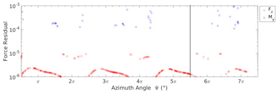
Figure 2.
Force residual as a function of simulation time history expressed in azimuth angles.
3. Results and Discussion
3.1. Coordinate System
The Cartesian coordinate systems used in the analysis are illustrated in Figure 3, namely the inertial coordinate and body-fixed coordinate. The inertial coordinate is stationary, while the body-fixed coordinate rotates and pitches along with the blade. The azimuth angle is defined as 0 at the minimum , and it increases counterclockwise. The pitch angle is defined as positive when the blade’s leading-edge is positioned to . We only use azimuth angle and pitch angle to describe the position and orientation of the blade, respectively. Hence, If not specified, x, y, and z are referred to the body-fixed coordinate system.
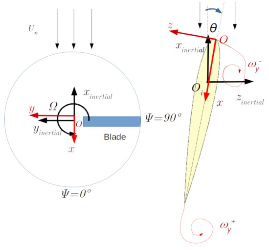
Figure 3.
Illustration of coordinate systems used in analysis: the Inertial coordinate, of which the origin is positioned at blade rotation/pitch center, and the body-fixed coordinate, of which the origin is at blade leading edge. All of the aerodynamic variables are defined according to the body-fixed coordinate.
3.2. Force and Moment
There is a marginal difference in both thrust and pitching moment coefficients in terms of the maximum values as shown in Figure 4. The stall event occurs later for the SST turbulence model, and the pitching-up moment in the post-stall phase is relatively smaller. This indicates differences of the detailed fluid structure in the stall regime; this will be studied in detail in the future but not within the scope of current study. Nevertheless, the overall trends of the curves are similar to each other, and we are using the numerical results of the SA turbulent model to illustrate the dynamic stall events on the rotating-pitching blade.
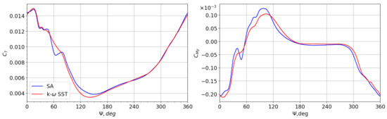
Figure 4.
Comparison of thrust and pitching moment coefficients of the blade within one revolution by different turbulence models: Spalart–Allmaras (SA) and the SST turbulence model.
Sectional force coefficients are shown in Figure 5 at radial locations = 0.607, 0.785 and 0.928. The plot shows an apparent difference between radial locations in both stall onset time and stalled value. Both and show an earlier stall for outboard locations. However, the extreme and stalled value of don’t take place at the outermost location. Both thrust and pitching moment curves in the post-stall phase oscillate distinguishably compared to their inboard counterparts.

Figure 5.
Sectional force coefficients at selected radial locations, = 0.607, 0.785 and 0.928. (a): sectional normal force coefficient ; (b): sectional pitch moment coefficient .
Figure 6 is the rotor map of both sectional normal force and moment coefficients. Force coefficients are non-dimensionalized by sound speed. The maximum appears in the region 0.6 < < 0.85, , which is in the pitching-down phase. While the relative high value (orange area) begins at , (pitching up) and remains until , (pitching down). The negative normal force also exists near blade tip at azimuth angle , which is a result of the tip vortex; it appears at the blade root as well, which is the attributed reverse flow region and the strong root whirl flow, the latter a pure result of the abrupt cut of the blade model at the root. The minimum (pitch down moment) appears at = 0.72, , which is in the pitching-down phase well beyond the maximum pitch angle. The relatively small value (blue region) starts from and ends near , which is consistent with the change of normal force, and this indicates that the dynamic stall occurs in this region. The maximum (pitching-up moment) appears at blade tip, , where a normal shock exists on the suction surface, see Figure 7 . is contoured with a bold line in the rotor map. The rugged line shows the recovery of occurs inboard first while very late at radial locations 0.6 < < 1.
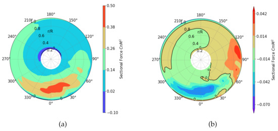
Figure 6.
Rotor map of sectional force coefficients. (a): sectional normal force coefficient normalised by sonic speed; (b): sectional pitch moment coefficient.
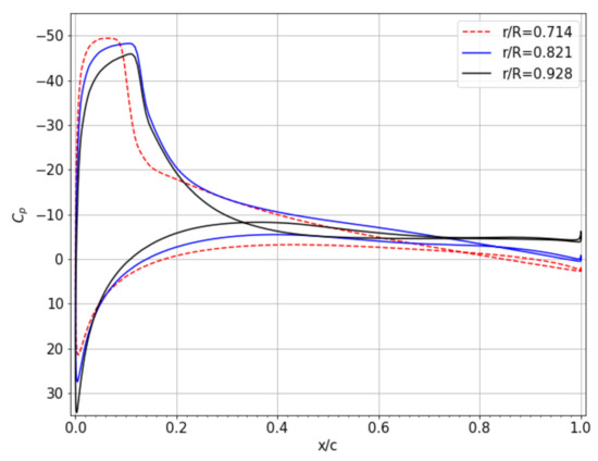
Figure 7.
Pressure coefficient of a slice on the blade at radial position = 0.714, 0.821 and 0.928, azimuth angle .
3.3. Vortex Structure
Since dynamic stall events are closely associated with the vortex generating and shedding on the upper surface of a blade, we show the vortex structures on the rotating blade at different azimuth angles in Figure 8. The location of vortex cores over the blade is plotted in Figure 9, which is extracted based on the eigenmodes of the velocity vectors [27]. This will be compared with previous research to illustrate the difference in rotating environment.
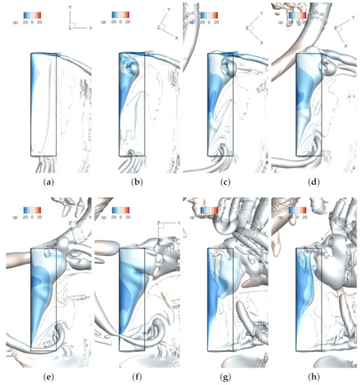
Figure 8.
Vortex structure shown by iso-surface of Q criterion () shaded by pressure coefficient cp referenced to forward flight speed. For each subplot, top: blade tip, bottom: blade root. The blade border is shown with the black rectangle. Azimuth positions: = (a) ; (b) ; (c) ; (d) ; (e) ; (f) ; (g) ; (h) . The inertial coordinate is plotted here.
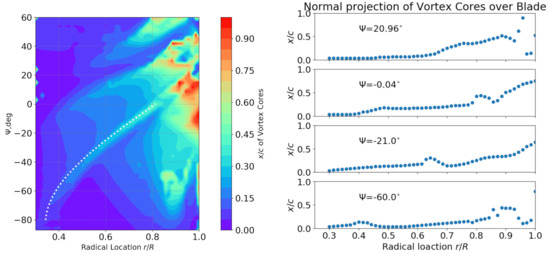
Figure 9.
Left: Location of the vortex cores over the blade in radical region evolving along azimuth. Dotted line is a curve , in rad. Right: Projection of vortex cores on the blade upper surface at selected azimuths.
An -shaped vortex structure is visible in the snapshots (b) (c) , which is similar to the observations for a pitching finite wing by [14], and also similar to what [15] called the -type arch vortex. A similar observation is also reported by [20]. Unlike on a pitching finite wing, as soon as the -shape vortex is shed, the leading edge vortex (LEV) comes into interaction with the blade tip vortex to a great extend, and even an inclined arch vortex appears at the tip, see (e) .
In order to see the interaction of the leading-edge vortex and the tip vortex, we take slices at several chord-wise locations near the tip region (0.94 < < 1.125), and integrate , in this region where , which is the main contribution to the tip vortex in cases that are free from strong interaction. The circulation in the y-direction indicates the mixture of LEV in the tip vortex region. This result is plotted in Figure 10 with selected azimuth angles.
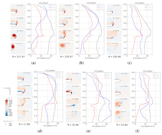
Figure 10.
Snapshots of the flood contour of vorticity field and the contour of in blade tip area (0.94 < < 1.125) at different chord-wise sections; The circulation , where S is the tip region where , . Azimuth positions: Ψ = (a) 318°; (b) 330°; (c) 357°; (d) 18°; (e) 36°; (f) 54°.
The consequent strong interaction of the LEV and tip vortex dominates the flow behavior of the post-stall phase. There are mainly four stages in this phase, symbolized by the shedding of LEV at the tip area. The 1st stage begins at , when the LEV accumulates at the blade-tip’s leading-edge, which is shown as the increasing integration of negative y circulation ; the LEV starts shedding at as the peak of moves rearward, and at the place where this peak locates, the circulation in the x-direction in the tip region is also relatively larger. As the separated DSV moves downstream and outboard, the tip vortex at is elevated and distorted. Alongside the rearward movement of , grows in the vicinity of the tip surface. This explains why the negative exists at the tip region on the rotor map of . The second stage begins at when the previous main DSV is transported off of the trailing edge; another LEV is accumulated at the leading edge. In this stage, the tip vortex at is no longer obvious, but the net circulation in the x-direction increases. This means, in the tip region that there exists a more diffused vorticity field rather than the conventional concentrated structure. As the LEV grows over the chord, the tip vortex is not apparent; nevertheless, it increases continuously in this area. From this time on, the LEV sheds and entrains the tip vortex, forming a large separation region over the tip area. Finally, marks the end of previous shedding of LEV and the beginning of the next shedding of LEV at the tip area. A reversely rotating tip vortex is generated beneath the mixture layer of the separated leading-edge vortex and tip vortex at . In the near wake, the tip vortex locates more outboard compared to the 1st stage, and a pair of counter rotating vortices is obvious. At azimuth , the interaction of LEV and tip vortex begins to disentangle at . Another growing and shedding of LEV at the tip area is observed, but in this stage there is no strong interaction with the tip vortex. It enters the recovery stage.
The interaction of the leading edge vortex with the tip vortex represents three important features:
- The leading-edge vortex is not “pinned” by the tip vortex, which is contrary to the observations for a pitching wing;
- There is a strong correlation of circulation in the x-direction and the chord-wise location of DSV. This can be explained as a result of lower pressure created by the DSV, which induced higher velocity around the tip.
- The concentrated tip vortex is entrained into LEV during the pitching-down phase, and a pair of counter-rotating vortices is observed in the near wake of the blade.
Ref. [28] measured the tip wake in the near field of an oscillating wing; he discovered the hysteresis behaviour of the tip vortex, and a more diffused tip vortex during a down-stroke compared with the up-stroke. Current numerical simulation complies with the observation of pitching wing.
Another significant feature shown in Figure 8 is the conical structured LEV on the rotating blade, which is very similar to the research on a rotating wing by [29]. This conical shaped structure is treated as a more stable LEV, “pinned” at the leading edge [30], if we look at slices taken along the chord-wise direction. Ref. [30] explains that the stability of LEV on rotating wing is due to the span-wise flow, which transports vorticity to the tip and inhibits the growth of LEV, hence the critical circulation beyond which the LEV will detach from the leading edge is not reached. In addition, this can explain the phenomenon observed by [17], who concluded that vortex evolution varies with radial positions on the blade, namely, at some locations, LEV sheds into dynamic stall vortex (DSV), while, in other places, only a secondary vortex is generated. When the phenomenon inspected from a three-dimensional perspective, this conclusion is just an incomplete description of the -shaped vortex outboard and the conical vortex structure inboard. That is to say, the detached DSV is rather a part of the arch vortex, which attaches to the blade surface with two “legs”; and this is due to the stability of the conical LEV structure in which no DSV is shed and observed inboard.
The special phenomenon of the rotating and pitching blade is the vortex generated inboard which can be seen in Figure 8b–f () as a swelling part within the conical LEV region inboard the blade, and it appears on different radial locations and grows in size while moving outboard. This swell structure creates a relative higher pressure on the blade, as is shown in Figure 11 where a shallow grey area at = 0.4875 is encompassed by a darker area. This is a result of the alleviated LEV, when compared with the one at = 0.625, where the LEV stays close to the upper surface of the blade. From the x plane slice, one can easily identify the detachment of the vortex structure. This structure corresponds to what [17] have observed on their retreating blade that inboard LEV didn’t generate a DSV but a secondary vortex. As the swell structure moves outboard, it carries the vorticity that arched away from the surface and hence at that radial location no shedding of the LEV occurs. The span-wise flow also contributes to the outboard moving of the swell structure.
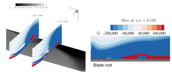
Figure 11.
The swell structure on the blade, represented with x and y slices. Left: slices at and ; Right: slice at .
This swell structure seems to be a result of the Coriolis force on the rotating blade at first thought, but we carefully examined the pressure force and the Coriolis force of the conical LEV slices at several spanwise locations and found out that the Coriolis force is too small to affect the vortex structure. The swell structure shown in Figure 8 exists at near the root corner, prior to the formation of the -type vortex. Indeed, the structure appears even earlier in this simulation at , but it doesn’t have any obvious effect on the pressure distribution on the blade’s surface. The growth, however, does have an impact on the pressure distribution later on as shown in Figure 11. The reason why this structure appears first inboard is still unclear. However, it cannot be explained by a relative stronger Coriolis force towards blade root at low Reynolds number: a greater magnitude inertial Coriolis force that pulls the LEV core away from the leading edge exists when the a rotating wing is positioned closer to the rotation axis [19]. We evaluated forces in the x-direction on the slices of the vortex structure, as shown in Figure 12a. Following the divergence theorem, we evaluated the pressure force on the slices of the vortex core:
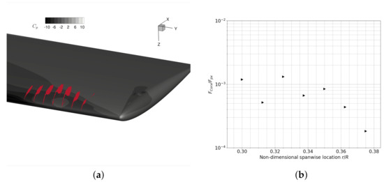
Figure 12.
Comparison of the pressure force and the Coriolis force in vortex cores. (a) area of integration, where ; (b) ratio of Coriolis force in the x-direction and pressure force in the x-direction .
The Coriolis force exerted on the vortex core can be evaluated as . The ratio of the Coriolis force to the pressure force is plotted in Figure 12b. At blade root, this value is as small as , and it decreases further as the non-dimensional spanwise location increases. Although increases with , this linear increase is not comparable to the quadratical increase of the pressure force, resulting in a continuously decreasing ratio as increases. It seems that, at such a high Reynolds number, the Coriolis force has little effect on the vortex core structure. Possible explanations for the emergence of the swell structure can be the effect of the jet-like radial flow itself or the upward flow at the blade root. Further research with a rotor hub or a winglet at root can help to clarify the mechanism of the vortex structure’s onset.
Since the position of the swell structure influences the sectional pitching moment, we thereby extracted the vortex cores and plot its x position against azimuth angle in Figure 9. The lighter color represents an aft position of the vortex core, which results in a negative pitching moment component. In Figure 5 at a radial location , , there is a small kink on both CnM2 and CmM2 curves; In Figure 9, we see that, at (or ), the vortex core at is located well beyond the line of the nearby LEV cores. The lighter color formed an edge in the contour map that represents the trajectory of the swell structure as it moves afterward as well as outward. We define this ridge as the position of the swell structure when (1) , (2) , in radial locations (3) , where is the scatter plot of the normal projection of the vortex cores on the blade in Figure 9. This value can be estimated as a quasi-uniform-acceleration movement on the blade:
The first term is the centrifugal effect, the second term is the contribution of the yawing effect, with representing a lower flow speed in vicinity of the blade’s upper surface, and the third term is the initial position of this vortex structure on the blade. In our case, the white dotted line in Figure 9 gives an approximation of the trajectory using the expression mentioned above for the movement, and .
3.4. Separation Points
The feature of dynamic stall is mainly the separation of the boundary layer, both at the trailing edge and the leading edge. Understanding, as well as modelling of dynamic stall need these separation points on the blade. Many methods, both Eulerian and Lagrangian, can be used to detect the flow separation in the unsteady flow. We present here pure Eulerian methods, the skin friction and shape factor criteria. The former theorem requiring wall shear stress is based on steady, laminar flows, but was recently extended by [31] to unsteady, turbulent and compressible flows; and the latter theorem requiring the near wall flow field is based on the boundary theory, and the separation criteria is proposed by [32] as for two-dimensional turbulent flows. We follow the rigorous skin friction criteria to extract the instantaneous separation points on the blade and then present the shape factor criteria resultant separation points to show how good the velocity field can be used to evaluate the separation points.
The skin friction lines are plotted in Figure 13 at selected azimuth angles. According to [33], the existence of a skin-friction line on a three-dimensional surface on which other lines converge is a necessary condition for the flow separation; and skin-friction line emerging from a saddle point indicates a global separation; otherwise, it is only a local separation. We don’t distinguish here global or local separation, since we know that the leading-edge vortex that attached to the blade can also contribute to such a local separation, which is our interest as well. For the a blade section at a radial position, the aforementioned criteria can be expressed mathematically:
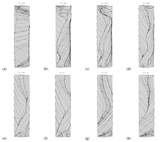
Figure 13.
Snapshots of the skin friction lines . For each subplot, the blade is placed the same way as in Figure 8, with the top side being blade tip and bottom being blade root, the left side being the blade leading edge, and the right side being the trailing edge. Azimuth positions are: = (a) (b) (c) (d) (e) (f) (g) (h) .
Similarly, if and , this is the point of attachment. We extract the sectional separation points and attachment points for the blade in a rotor map in Figure 14. Note that the stagnation point is also an attachment point, hence we have excluded this point in our algorithm. The leading-edge separation of boundary layer starts outboard and inboard both at , while, at mid-span , this starts at . Together with the attachment points, we see that, between azimuth angle and , the flow re-attaches immediately beyond the separation points, which indicates the existence of attached leading edge vortex. When the blade enters the 3rd quadrant, the attachment points begin to move downstream, but the starting azimuth is highly dependent on the radial location. For example, at , the vortex begins to grow leeward very early while, at , the vortex remains at the leading edge for a long time. Note that the growth of LEV starts at both ends of the blade and propagates toward mid-span. A helicopter blade may not show the same character, for example simulation by [21], shows a rather inboard to outboard propagation of the growth of LEV, in which 7A rotor has a linear twist −8.3deg/R meaning larger pitch angle inboard. In our case, the pitch angle is the same for different radial stations, and we observed a double directional propagation of the growth of LEV. Ref. [24] mentioned that, in the vicinity of wing tip, the flow is attached due to tip vortex induced flow as the wing pitches. In our case, this holds for the azimuth angles before . We have already seen in Figure 10 that there exists a strong correlation of tip vortex strength and the leading edge vortex strength , and it is indeed this interaction of LEV with tip vortex makes the LEV no longer staying attached at tip. At , we see a light-coloured region out board, where the separation occurs between and , far away from the other leading edge separation positions. In Figure 15, we show the Mach contour, pressure coefficient and skin-friction coefficient in the x-direction at radial location at this azimuth angle. On the upper surface of the blade section, drops from positive to negative and crosses 0 at , where the shows a sharp decrease. This separation is obviously a product of shock wave. Based on the discussion above, we can categorise the rotor map into four regions, namely fully attached region (F.A.), leading-edge separation region (L.S.), fully separated region (F.S.) and a shock induced separation region (SI). These regions are plotted in Figure 16.
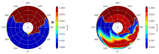
Figure 14.
Rotor map of chord-wise separation and attachment locations. The direction of the free stream is from to , and the rotating direction is counterclockwise.
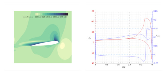
Figure 15.
Mach contour of the slice and the corresponding pressure coefficient , skin-friction in the x-direction on the blade section, azimuth angle . On the upper surface, drops from positive to negative and crosses 0 at , where the shows a sharp increase.
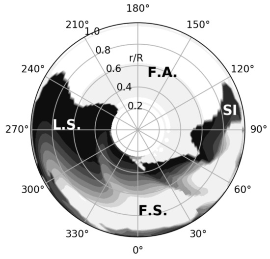
Figure 16.
Rotor map of separation regions. F.A. is the fully attached region; L.S. is the leading edge separated region, where the LEV is attached, representing as the conical vortex structure on the rotating blade; F.S is the fully separated region due to the shedding of DSV; SI is the shock induced separation region.
Another separation criterion that can be used (see [21]) to detect separation in turbulence flows is based on the shape factor , namely the ratio of the momentum thickness over displacement thickness of the boundary layer for a two-dimensional flow, as illustrated in Figure 17:
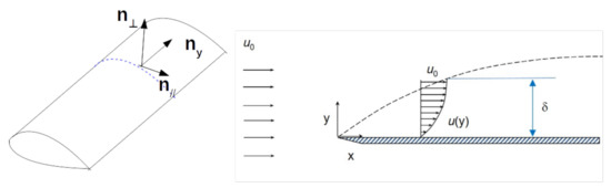
Figure 17.
left: Illustration of coordinate system used to post-process shape factor; right: schematics of boundary layer over a flat plate.
Ref. [32] stated that is characteristic of the boundary separation, yet they did not give a sufficient criteria. In order to imply the concept on our rotating blade, we transformed all the velocity to the blade-section-fixed coordinate and dealt with the velocity parallel to the airfoil at different radial sections, as shown in Figure 17, along direction. The flow along radial direction is not considered when analysing the shape factor since observing from the blade, and the main component of the flow is perpendicular to the leading edge of the blade. The outer edge of the boundary layer is treated as the location where the velocity reached its maximum along the direction. To determine how good this criterion can predict separation using only velocity field, we plot in Figure 18 the shape factor and the skin-friction in the x-direction at azimuth position . The lower bound shows quite a good agreement with the x skin-friction contour on the blade surface. However, Ref. [32] shows only the correlation of separation and shape factor H in turbulent boundary layers, the utilisation of such criteria to detect separation should be considerably careful.
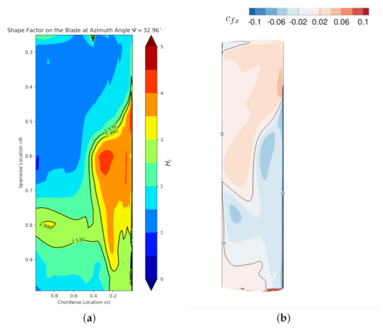
Figure 18.
(a) Shape Factor on the upper surface at azimuth angle , two contour lines indicate the upper and lower bound of value to determine the separation; (b) skin friction on the upper surface at azimuth angle , the 0 contour line showing the separation line.
3.5. Comparison of Stall Events on a Pitching Airfoil and a Section of the Rotating Blade
In order to understand the differences of dynamic stall between a rotating blade section and a pitching airfoil with the same harmonic pitching, the force coefficients and the Q contours of both cases are plotted in Figure 19. This spanwise location is exactly the center of the -type dynamic stall vortex. The numerical investigation of a pitching airfoil satisfying Equation (1) is explained in detail by [34]. The main differences between the pitching airfoil (2D case) and the section of the three-dimensional rotating blade (3DR case) include: (1) the magnitude of the force coefficients (both and ) differ significantly in the pitching-up phase; (2) the onset of the moment stall of the pitching airfoil is, in terms of the pitch angle, earlier than the blade section. However, the curves are quite close in the pitching-down phase for both cases and the normal force stall occurs almost simultaneously.
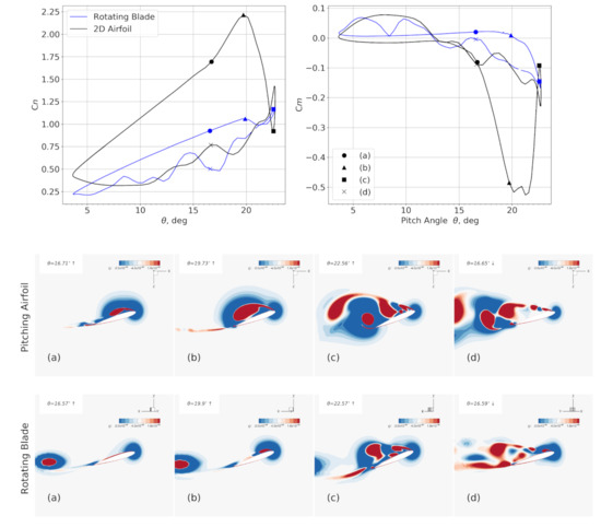
Figure 19.
Up: Comparison of Sectional force coefficients on blade at with the numerical simulation of non-rotating pitching blade and pitching airfoil. Down: vortical structure on pitching airfoil and the slice at radial location = 0.898 of the rotating blade, shown as a contour of Q at selected pitch angles shown in the force plot. For rotating blade, these pitch angles correspond to azimuth angle (a) , (b) , (c) , (d) . The coordinate in the slice of the rotating blade is the inertial one.
The maximum normal force coefficient of the airfoil is 2.21 while the value of the blade section is only 1.16. In the process when the leading-edge vortex grows, there is an obvious increase of the slope , while this is not observed on the blade section. The normal force stalls for both cases are near , and, in the post-stall stage, normal force coefficients are relative close to each other. The extreme value of the moment coefficient of the 2D case is −0.52, while the counterpart on the rotating blade is only −0.145. The moment stall of the blade section lags behind that of the pitching airfoil, and is relatively milder.
Comparing the vortical structures at different dynamic stall stages, there seems to be a delayed LEV growth from (a) to (c). When the LEV is quite obvious on the pitching airfoil, the LEV is unable to be seen on the blade section at time (a). Time (b) for both cases are the stages before the shedding of LEV. However, both Q contours are comparable to each other at time (c), with both of them representing the aft-moving dynamic stall vortex. We see here that there is no phase of growing LEV on the blade section, as seen in time (b) of the 2D case. It seems that, at the moment when the LEV appears on the blade section, it pinches off immediately and moves aft-ward, which is significantly different from what happens on the 2D pitching airfoil. This strange behaviour of the LEV on the blade section is a consequence the following factors: (1) the effect of the induced velocity field in the rotating environment, which yields a smaller effective angle of attack (AoA) , and hence results in the delayed effect on the moment stall; (2) the outward transportation of y vorticity by the radial flow, which reduces the strength of the leading-edge vortex, and results in the lack of growth phase of the LEV on the blade section; (3) the -type vortex structure, which arches itself away from the surface, moves aft-ward and allows the vorticity that is transported from inboard to form a new LEV, and hence results in a strong increase in and a mild decrease of after the detachment of the LEV. Time (d) shows the pitching-down phase, where the vortex structures are similar to each other, apart from an obvious vortex in the vicinity of the blade section’s trailing edge. This is a consequence of the aforementioned factor (2): this vortex is transported from inboard. Moreover, the trailing-edge vortex on the blade section is more diffusive than the pitching airfoil.
The vorticity of the counter-clockwise rotating vortex over the upper surface of the airfoil in Figure 19 is integrated and plotted in Figure 20. This value interprets the strength of the LEV or DSV when the leading-edge separation occurs. The two curves have a similar trend, in the upward pitching phase, the curve of the circulation is quite flat. Then, after a light decrease they surge up and in the downward pitching phase, they attenuate in oscillation. There are still three major differences:
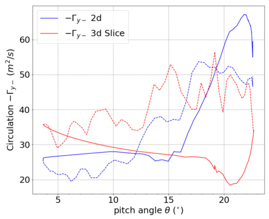
Figure 20.
Vorticity strength of the counter-clockwise vortex over the upper surface of the pitching airfoil and the slice of the rotating blade, with solid lines representing the upward pitching and dashed lines the downward pitching. The circulation , and in region S, .
- (1)
- The maximum circulation of the DSV in 2D case is larger;
- (2)
- The oscillation of the 2D case in the downward pitching scenario is milder and the DSV strength of the 2D case is obviously smaller;
- (3)
- There is a delay of 5.2 for the 3D rotating blade case when comparing the point of which the leading edge vortex begins to grow.
The first point can be explained as the lack of a third dimension for the vortex to grow, resulting in a concentration of vorticity. The second point can be explained as the continuing transportation of the vorticity from inboard, where the swell structure grows with the radial flow on the blade, as shown in Figure 9. At azimuth angle , the circulation of the 3D slice is clearly larger, which is also the effect of the continuous transportation of vorticity from inboard. Figure 16 shows that, at this azimuth angle, the leading-edge separation still exists inboard. The third point can be explained as the combined effect of the induced velocity field in the rotating environment and the outward transportation of vorticity by the radial flow. The induced velocity field means that the effective angle of attack on a rotor blade is different from that on a pitching airfoil: ; Additionally, the outward transportation of vorticity means that, unless an increase of is present, the circulation over the blade section will not increase. Here,
“” is the side of the blade section towards root, and "" is the side of the blade section towards tip.
Blade element momentum theory (BEMT) is the lower order model that is widely used to predict the loads on the rotor disk. The in-flow sub-model is used for determining the effective angle of attack (AoA) for the blade elements. If we take the Drees linear inflow model [35] and implement the momentum analysis on the rotor for our case, we can get the modelled induced AoA as shown in Figure 21a,b. At the radial location , the induced AoA has a maximum value of 2.6, which is smaller than 5.2 . Hence, the evaluation of transported circulation is another modelling factor to relate the stall event on the blade section to that on the pitching airfoil.
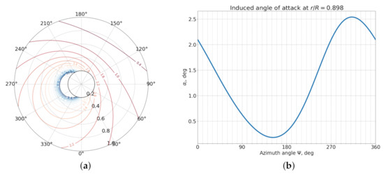
Figure 21.
Induced AoA according to BEMT, ; (a) rotor map of ; (b) at .
4. Conclusions
A numerical investigation with URANS using SA and SST turbulence models was carried out on a single rotating flat rectangular blade with a NACA 0012 airfoil, and the flow feature of the SA result was researched in detail. The collective controls were chosen in order to create dynamic stall on the retreating blade, and the cyclic control was acquired with CAMRADII with the minimum-lateral-moment trim condition. Several features not yet reported in previous research were found.
- A strong interaction of the DSV and the tip vortex was observed and described in detail for this case. Contrary to observations of a pitching wing, the LEV on a rotating pitching blade is not pinned by the presence of the tip vortex, but rather the shedded DSV drastically interacts with the tip vortex, yielding a pair of counter rotating vortices in the near wake; the slices also indicate a diffused tip vortex in the near wake, whether this diffusion is caused by the pure pitch-down effect as observed for the pitching wing or if it is further diffused by the interaction of the tip vortex is not yet clear.
- Despite an -shaped vortex outboard, a swell vortex structure is observed to generate mostly inboard and moves outboard while gaining vorticity and size, which plays an important role after the shedding of the first DSV.
- The presence of the swell structure is not an outcome of the Ro effect inboard, contrary to the respective low Reynolds number counterparts. The Coriolis force is three orders of magnitude smaller than the pressure force, and hence unable to be the main cause. The mechanism of the onset of the swell structure is not yet clear.
- By tracing the vortex cores over the suction side of the blade, we proposed to use a quasi-uniform-acceleration movement to describe the position of the swell structure, and the parameters were given for this special case.
- By comparing the force coefficients on an outboard radial location with pitching airfoil, we show that a large difference exists between the two cases. The induced velocity field of the rotating environment, the radial flow due to the centrifugal effect, and the 3D effect created -shape vortex altogether caused a simultaneous normal force stall and a delayed and mild moment stall on the blade section. The 2D simulation showed a stronger dynamic stall vortex that magnified both the normal force and the moment.
- By integrating the counter-clockwise rotating vorticity above the upper surface of the pitching airfoil and blade section, we showed the strong circulation in the recovery stage of the latter case, which is a consequence of the outward transportation of vorticity by the radial flow. The aforementioned swell structure also plays an important role when it crosses the blade section. The delayed increase of the circulation is assumed to be a result of the induced velocity field in the rotating environment and the transportation of vorticity due to the radial flow.
Based on the conclusions above, a more complex and unique vortex system exists on a pitching rotating blade. We thus suggest that, in order to model dynamic stall more precisely force modelling over a rotating blade, a better 3D vortex model is needed in addition to the blade-element-momentum theorem. Adjusting modelling parameters according to 2D pitching airfoil numerical simulations or experiments may not improve the accuracy of the model in predicting loads of a rotating blade.
Author Contributions
Conceptualization, Numerical Simulation, and Validation, Y.R.; Review and supervision: M.H. All authors have read and agreed to the published version of the manuscript.
Funding
This research was funded by the China Scholarship Council.
Institutional Review Board Statement
Not applicable
Informed Consent Statement
Not applicable
Data Availability Statement
Not applicable
Conflicts of Interest
The authors declare no conflict of interest.
Abbreviations
List of symbols and abbreviations used in this manuscript:
| a | sound speed, m/s |
| c | chord length, m |
| chord-wise position, 0 at leading edge and 1 at trailing edge | |
| pitch angle of the blade, deg | |
| ,, | Collective pitch angle, lateral cyclic pitch |
| and longitudinal cyclic pitch respectively, deg | |
| azimuth angle, equaling 0 when the blade reaches most rearward position | |
| parallel to the inflow, and increases counter-clockwise, deg | |
| thrust coefficient, , where T is the thrust, acting perpendicular | |
| to the rotor disk, N | |
| pitch moment coefficient, , where is the pitch moment | |
| on the rotor, | |
| air density | |
| T | temperature, K |
| rotational speed, rad/s | |
| R | rotor radius, m |
| normalized radial position, 0 at rotation centre and 1 at blade tip | |
| forward flight speed, m/s | |
| advance ration, | |
| spacing or grid length, m | |
| sectional normal force coefficient, , where n is the sectional | |
| normal force, is the local relative airspeed, or , | |
| sectional moment force coefficient, , where m is the sectional | |
| pitch moment, | |
| M | mach number, |
| p | pressure, Pa |
| pressure coefficient, , where is the ambient pressure | |
| Q | the second invariant of the velocity gradient tensor |
| , | vorticity in x and y direction of the blade fixed coordinate, x positive from |
| leading edge to trailing edge, and y positive from blade tip to blade root, | |
| , | circulation in x and y direction, , where S is a specific region |
| to perform integration, | |
| Coriolis force, , where is the velocity along the y | |
| direction of body-fixed coordinate, N | |
| pressure force, , where is the normal vector of a closed | |
| surface S, pointing out of the control volume, N | |
| shape factor at a point on the blade surface | |
| skin friction coefficient in x direction of blade fixed coordinate | |
| effective angle of attack, deg | |
| induced velocity due to rotating environment, positive toward the pressure | |
| side of the rotor | |
| induced angle of attack, positive when the leading edge of a blade section | |
| rotates towards the pressure side of the rotor, deg | |
| SA model | Spalart–Allmaras turbulence model |
| LEV | leading edge vortex |
| TEV | trailing edge vortex |
| DSV | dynamic stall vortex |
| 2D | 2 dimensional |
| 3D | 3 dimensional |
| 3DR | 3 dimensional rotating |
| AoA | angle of attack |
| BEMT | blade element momentum theory |
Appendix A. Grid Convergence Study
In order to show the convergence of current grid, we created a coarse grid and medium grid with the same strategy as described in Section 2.1, and we list the spacing of each block for these grids in Table A1. is the average of the edge length among the cells, and is the average of the cell volumes. During coarsening the original fine grid, we keep the height of the first layer off the blade surface having the same value which satisfies . In addition, the number of connectors in three directions are all reduced according the level of the coarse grid. We present here only simulations with the Spalart–Allmaras turbulence model.
Table A1.
Grid spacings and numerical results.
Table A1.
Grid spacings and numerical results.
| Coarse Grid | Medium Grid | Fine Grid | |
|---|---|---|---|
| Pitch Block | ; | ; | ; |
| Rotating Block | ; | ; | ; |
| Far-field Block | ; | ; | ; |
| 0.00782 | 0.00793 | 0.00791 |
We choose the average of cell edge lengths in pitch block as the spacing indicator, and following [36], we can obtain the exact value of a partial differential equation as:
where c is a constant and h is some measure of grid spacing, p is the order of convergence. We plot the grid convergence curve in Figure A1. The fitted curve of Equation (A1) is , which means the grid has an order of convergence of 1.566. We have used a 2nd order scheme for both mean-flow flux and turbulence flux with a Spalart–Allmaras model; theoretically, this value should be 2. Based on Equation (A1), the exact value of is 0.007942, and the current grid has an error of . The superposition of and in different revolutions is plotted in Figure A2, and we can see that, after the 3rd revolution, the forces have already converged to a good extent. We have compared the average and of the SA model and the Menter SST model, and found that is exactly the same, while the averaged for SA model is −0.001328, and, for model, it is −0.001676.

Figure A1.
Grid convergence study with coarse, medium, and fine grids.

Figure A2.
Superposition of force coefficients of different revolutions.

Figure A3.
Configuration of the mesh for validation: (a) blade block; (b) voxel farfield block.

Figure A4.
Thrust coefficient along inner iterations.

Figure A5.
Pressure coefficient at different span-wise locations on the blade: comparison between numerical simulation with Spalart–Allmaras turbulence model and experiment result [37])

Figure A6.
Iso-surface of Q-criterion (Q = 5000 s) contoured with vorticity magnitude and super-positioning on y-sliced mesh.
Appendix B. Validation of grid strategy and turbulence model on the hovering case
The Caradonna–Tung rotor model is adopted, and the surface mesh follows the same space criteria as described in Section 2.1. The only difference of the blade block is the root part, where unstructured pyramids’ prisms and tetrahedra are used, as shown in Figure A3a. The farfield block consists of a region that is uniformly spaced as the rotating block in current simulation and the voxel grid growing from small to large scale on a farfield boundary. The region right below the rotor is refined with a point source in order to catch tip vortex trajectories, as shown in Figure A3b. The flow condition is summarised in Table Table A2, and the comparison of grid for the simulation and validation case are summarised in Table Table A3. The numerical method for the hovering case is the same as the current simulation, except that the rigid motion herein includes only rotation of the whole block. The Spalart–Allmaras turbulence model is adopted. Figure A4 shows the thrust coefficient along the simulation revolutions, and Figure A5 shows the comparison of the pressure coefficients on = 0.5, = 0.8, = 0.96 span-wise locations. Figure A6 shows the tip vortex trajectory using Q-criterion shaded with vorticity magnitude.
Table A2.
Flow condition for validation.
Table A2.
Flow condition for validation.
| Chord length c (m) | 0.195 |
| Aspect Ratio AR | 6 |
| Tip Mach number, | 0.877 |
| Tip Reynolds number | |
| Tip velocity (m/s) | 299.24 |
| Collective pitch | 8 |
| Angular Velocity (rad) | 255.76 |
Table A3.
Comparison of the spatial resolution between current simulation and validation case.
Table A3.
Comparison of the spatial resolution between current simulation and validation case.
| Current Simulation | Validation Case | |
|---|---|---|
| N around airfoil | 364 | 308 |
| N over the blade span/AR | 55.25 | 33.67 |
| N inside the boundary layer at midchord and = 0.8 | 56 ( mm) | 68( mm) |
| Max y+ | 0.55 | 0.9 |
| at LE | 0.133% | 0.2% |
| max chord-wise | 1.3% | 1.43% |
| max normal to wall | 4.6% | 3.39% |
The thrust coefficient of the experiment is , and the validation case gives a value of 0.00566, which is 19.6% larger than experiment data, which is consistent with the pressure coefficient, where, at = 0.8, the maximum has an error of 11.55%. Comparing the simulation result of the hover case with the Experiment data from [37], we conclude that the SA turbulence model is capable of qualitatively catching the main characteristic of the pressure distribution on the blade in rotation environment, and the voxel grid with point source as refinement is able to keep track of the tip vortex outside the fine grid region. The same mesh strategy and turbulence utilised for the current simulation is thus considered to give a close estimation of the flow phenomena on the pitching rotating blade.
References
- Martin, J.M.; Empey, R.W.; McCroskey, W.J.; Caradonna, F.X. An experimental analysis of dynamic stall on an oscillating airfoil. J. Am. Helicopter Soc. 1974, 19, 1:26–1:32. [Google Scholar] [CrossRef]
- McCroskey, W.J.; Carr, L.W.; McAlister, K.W. Dynamic stall experiments on oscillating airfoils. AIAA J. 1976, 14, 1:57–1:63. [Google Scholar] [CrossRef]
- Dadone, L.U. Two-Dimensional Wind Tunnel Test of an Oscillating Rotor Airfoil; National Aeronautics and Space Administration: Washington, DC, USA, 1977; Volume 1. [Google Scholar]
- McAlister, K.W.; Carr, L.W.; McCroskey, W.J. Dynamic Stall Experiments on the NACA 0012 Airfoil; National Aeronautics and Space Administration: Washington, DC, USA, 1978. [Google Scholar]
- Sankar, N.L.; Tassa, Y. Compressibility Effects on Dynamic Stall of an NACA 0012 Airfoil. AIAA J. 1981, 19, 557–558. [Google Scholar] [CrossRef]
- Walker, J.M.; Helin, H.E.; Strickland, J.H. An experimental investigation of an airfoil undergoing large-amplitude pitching motions. AIAA J. 1985, 23, 8:1141–8:1142. [Google Scholar] [CrossRef]
- Carr, L.W. Progress in analysis and prediction of dynamic stall. J. Aircr. 1988, 25, 6–17. [Google Scholar] [CrossRef]
- Ekaterinaris, J.A.; Platzer, M.F. Computational prediction of airfoil dynamic stall. Prog. Aerosp. Sci. 1998, 33, 759–846. [Google Scholar] [CrossRef]
- Guilmineau, E.; Patrick, Q. Numerical study of dynamic stall on several airfoil sections. AIAA J. 1999, 37, 1:128–1:130. [Google Scholar] [CrossRef]
- Geissler, W.; Dietz, G.; Mai, H. Dynamic stall on a supercritical airfoil. Aerosp. Sci. Technol. 2005, 9, 5:390–5:399. [Google Scholar] [CrossRef]
- Spentzos, A.; Barakos, G.; Badcock, K.; Richards, B.; Wernert, P.; Schreck, S.; Raffel, M. Investigation of three-dimensional dynamic stall using computational fluid dynamics. AIAA J. 2005, 43, 5:1023–5:1033. [Google Scholar] [CrossRef]
- Lorber, P. Tip vortex, stall vortex, and separation observations on pitching three-dimensional wings. In Proceedings of the 23rd Fluid Dynamics, Plasmadynamics, and Lasers Conference, Orlando, FL, USA, 6–9 July 1993; p. 2972. [Google Scholar]
- Le Pape, A.; Pailhas, G.; David, F.; Deluc, J.M. Extensive Wind Tunnel Tests Measurements of Dynamic Stall Phenomenon for the OA209 Airfoil Including 3D Effects; Vertical Flight Society: Fairfax, VA, USA, 2007. [Google Scholar]
- Kaufmann, K.; Costes, M.; Richez, F.; Gardner, A.D.; Pape, A.L. Numerical investigation of three-dimensional static and dynamic stall on a finite wing. Vert. Flight Soc. 2015, 60, 3:1–3:12. [Google Scholar] [CrossRef]
- Visbal, M.R.; Garmann, D.J. High-fidelity simulations of dynamic stall over a finite-aspect-ratio wing. In Proceedings of the 8th AIAA Flow Control Conference, Washington, DC, USA, 13–17 June 2016; p. 4243. [Google Scholar]
- Kaufmann, K.; Merz, C.B.; Gardner, A.D. Dynamic stall simulations on a pitching finite wing. J. Aircr. 2017, 54, 1303–1316. [Google Scholar] [CrossRef]
- Raghav, V.; Komerath, N. Velocity measurements on a retreating blade in dynamic stall. Exp. Fluids 2014, 55, 1669. [Google Scholar] [CrossRef]
- Wen, G.; Gross, A. Numerical Investigation of Dynamic Stall for a Helicopter Blade Section. In Proceedings of the 2018 AIAA Aerospace Sciences Meeting, 8–12 January 2018; Kissimmee, FL, USA; p. 1557. [Google Scholar]
- Smith, D.T.; Rockwell, D.; Sheridan, J.; Thompson, M. Effect of radius of gyration on a wing rotating at low Reynolds number: A computational study. Phys. Rev. Fluids 2017, 2, 064701. [Google Scholar] [CrossRef]
- Letzgus, J.; Gardner, A.D.; Schwermer, T.; Keßler, M.; Krämer, E. Numerical investigations of dynamic stall on a rotor with cyclic pitch control. J. Am. Helicopter Soc. 2019, 64, 1:1–1:14. [Google Scholar] [CrossRef]
- Richez, F. Analysis of dynamic stall mechanisms in helicopter rotor environment. J. Am. Helicopter Soc. 2018, 63, 2:1–2:11. [Google Scholar] [CrossRef]
- Johnson, W. CAMRAD II, Comprehensive Analytical Model of Rotorcraft Aerodynamics and Dynamics; Release 4.9; Johnson Aeronautics: Palo Alto, CA, USA, 2012. [Google Scholar]
- Schwamborn, D.; Gardner, A.D.; von Geyr, H.; Krumbein, A.; Lüdeke, H.; Stürmer, A. Development of the DLR TAU-code for aerospace applications. In Proceedings of the International Conference on Aerospace Science and Technology, Bangalore, India, 26–28 June 2008; pp. 26–28. [Google Scholar]
- Costes, M.; Richez, F.; Le Pape, A.; Gavériaux, R. Numerical investigation of three-dimensional effects during dynamic stall. Aerosp. Sci. Technol. 2015, 47, 216–237. [Google Scholar]
- Li, G.H.; Wang, F.X. Evolution characteristic analysis of double-helical vortex wake of high Reynolds number flow. Acta Phys. Sin. 2018, 67, 054701. [Google Scholar]
- Singh, K.; Páscoa, J.C. Numerical modeling of stall and post stall events of a single pitching blade of a cycloidal rotor. J. Fluids Eng. 2019, 1, 141. [Google Scholar]
- Sujudi, D.; Haimes, R. Identification of swirling flow in 3D vector fields. In Proceedings of the 12th Computational Fluid Dynamics Conference, San Diego,CA,USA, 19–22 June 1996; p. 1715. [Google Scholar]
- Chang, J.W.; Park, S.O. Measurements in the tip vortex roll-up region of an oscillating wing. AIAA J. 2000, 38, 6:1092–6:1095. [Google Scholar] [CrossRef]
- Ozen, C.A.; Rockwell, D. Three-dimensional vortex structure on a rotating wing. J. Fluid Mech. 2012, 707, 541–550. [Google Scholar] [CrossRef]
- Ellington, C.P.; Van Den Berg, C.; Willmott, A.P.; Thomas, A.L.R. Leading-edge vortices in insect flight. Nature 1996, 384, 626–630. [Google Scholar] [CrossRef]
- Haller, G. Exact theory of unsteady separation for two-dimensional flows. J. Fluid Mech. 2004, 512, 257–311. [Google Scholar] [CrossRef]
- Castillo, L.; Wang, X.; George, W.K. Separation criterion for turbulent boundary layers via similarity analysis. J. Fluids Eng. 2004, 126, 297–304. [Google Scholar] [CrossRef]
- Tobak, M.; Peake, D.J. Topology of three-dimensional separated flows. Annu. Rev. Fluid Mech. 1982, 14, 1:61–1:85. [Google Scholar] [CrossRef]
- Avanzi, F. Analysis of Dynamic Stall on a Pitching Airfoil with Spectral Proper Orthogonal Decomposition. Master’s Thesis, Universita Degli Studi Di Padova, Padova, Italy, 2019. [Google Scholar]
- Leishman, G.J. Principles of Helicopter Aerodynamics; Cambridge University Press: New York, NY, USA, 2006; pp. 158–160. [Google Scholar]
- Oberkampf, W.L.; Trucano, T.G. Verification and validation in computational fluid dynamics. Prog. Aerosp. Sci. 2002, 38, 3:209–3:272. [Google Scholar] [CrossRef]
- Caradonna, F.X.; Tung, C. Experimental and Analytical Studies of a Model Helicopter Rotor in Hover. 6th European Rotorcraft and Powered Lift Aircraft Forum; Bristol, UK: New York, NY, USA, 16–19 September 1980; pp. 25:1–25:19. [Google Scholar]
Publisher’s Note: MDPI stays neutral with regard to jurisdictional claims in published maps and institutional affiliations. |
© 2021 by the authors. Licensee MDPI, Basel, Switzerland. This article is an open access article distributed under the terms and conditions of the Creative Commons Attribution (CC BY) license (http://creativecommons.org/licenses/by/4.0/).