OpenAP: An Open-Source Aircraft Performance Model for Air Transportation Studies and Simulations

Abstract

Air traffic simulations serve as common practice to evaluate different concepts and methods for air transportation studies. The aircraft performance model is a key element that supports these simulation-based studies. It is also an important component for simulation-independent studies, such as air traffic optimization and prediction studies. Commonly, contemporary studies have to rely on proprietary aircraft performance models that restrict the redistribution of the data and code. To promote openness and research comparability, an alternative open performance model would be beneficial for the air transportation research community. In this paper, we introduce an open aircraft performance model (OpenAP). It is an open-source model that is based on a number of our previous studies, which were focused on different components of the aircraft performance. The unique characteristic of OpenAP is that it was built upon open aircraft surveillance data and open literature models. The model is composed of four main components, including aircraft and engine properties, kinematic performances, dynamic performances, and utility libraries. Alongside the performance model, we are publishing an open-source toolkit to facilitate the use of this model. The main objective of this paper is to describe each main component, their connections, and how they can be used for simulation and research in practice. Finally, we analyzed the performance of OpenAP by comparing it with an existing performance model and sample flight data.

1. Introduction

Many current air traffic management studies are aimed at solving the challenges caused by the increasing demand for air transportation. In the likely future scenario wherein air transportation is continuously being utilized more, innovative strategies will have to be investigated to maintain the safety and efficiency of flights, while keeping up with the growing capacity demand. To evaluate different concepts, large-scale air traffic simulations with future air traffic density need to be undertaken. Though several commercial air traffic simulators exist, the growing demand for more transparency in research data and research tools has made the open-source option stand out. For example, BlueSky [1], an open-source air traffic simulator, has become popular in the air traffic management research community.

Among other things, the aircraft performance model constitutes a core part of traffic simulators. The domain of aircraft performance or flight mechanics studies characteristics of aircraft such as speed, altitude, thrust, drag, and fuel consumption. Based on the aircraft dynamic model, it provides methods with which to compute flight trajectories. Many air traffic management studies are dependent on the aircraft performance model. Currently, many of these studies depend on the proprietary model Base of Aircraft Data (BADA), including BADA 3 and BADA 4 [2,3]. No comparable open alternative to BADA is available. One also developed by Eurocontrol, the General Aircraft Modelling Environment (GAME) is a kinematic-only performance model [4] that can be used for air transport research. Compared to BADA, it is less frequently used by air transport researchers. Previous research in [5] has produced a simplified aircraft performance model, named COALA, which uses part of the BADA model data. From the aviation industry, almost all aircraft manufacturers provide commercial performance data and tools for their aircraft. For example, Airbus has developed the Performance Engineering Programs (PEP) [6] that can be used as a standalone software tool. In addition, third-party commercial tools that model aircraft performance also exist. One of the examples is PIANO software [7].

Due to the proprietary nature of these models and tools though, users are limited by the strict license agreements, which makes it difficult to redistribute and to use the models commercially or openly. For open-source projects like BlueSky, lacking a performance model that can be redistributed would pose a challenge for sharing the tool as a complete open simulator. In earlier research, we built a preliminary performance model that is purely based on models from the literature [8]. However, the lack of up-to-date information led to the research completed in this paper.

In this paper, we present an open aircraft performance model, OpenAP, which can be used as an alternative to BADA for future air traffic management studies. It is a model produced by the combination of open data, literature models, and estimated parameters originating from open data. The processes of obtaining different model components have been previously published by the authors, which are discussed and summarized in later sections. Our final goal is to provide an open model that can be used, distributed, and modified freely under an open-source license. Additionally, a toolkit is to be published alongside this paper (available at: https://github.com/tudelft-cns-atm/openap). The OpenAP toolkit includes both the model data and the python code libraries. It thus allows quick access and model integration in potential applications.

The results presented in this paper largely benefit from the recently expanded adoption of automatic dependent surveillance-broadcast (ADS-B) and Enhanced Mode-S (EHS) technologies. A large quantity of flight data is transmitted by aircraft through these surveillance methods. This data can be freely received by researchers. With this open surveillance data, new opportunities for data-driven modeling emerge. Previous studies have proven the potential of the data-driven method using flight data. Some examples of these studies involve inferring aircraft mass [9,10], filtering and estimating flight states [11], modeling fuel consumption [12], and predicting the performance [13].

For instance, one of the data-driven components in OpenAP is the aircraft kinematic performance model, which is a result of our earlier study [14,15]. The kinematic model deals with parameters such as aircraft speed, altitude, vertical rate, and distances. These parameters can be directly observed from surveillance data. By deploying adequate data mining and estimation methods at different phases of flight, the kinematic performance can be accurately modeled. However, a data-driven approach is not suitable for most of the dynamic performance components, since there are often too many unknowns to solve given the limited set of equations and observables from flight data. The aircraft thrust and fuel flow are two examples. In these cases, we must address the modeling challenge based on engine performance instead of flight data. Literature models and other open data are used for thrust and fuel flow. In general, modeling the dynamic performance components (thrust, drag, and fuel flow) is a crucial component of the studies that led to the publishing of OpenAP.

In the following section of the paper, the details of the different OpenAP components are described. In Section 2, the basis of the OpenAP model and toolkit is explained. In Section 3, the aircraft and engine property model is discussed. In Section 4 and Section 5, the kinematic and dynamic performance models are presented respectively. Other related utility libraries are shown in Section 6. In Section 7, examples and demonstrations of OpenAP are presented. In sections eight and nine, discussion and conclusions are presented.

2. OpenAP Building Blocks

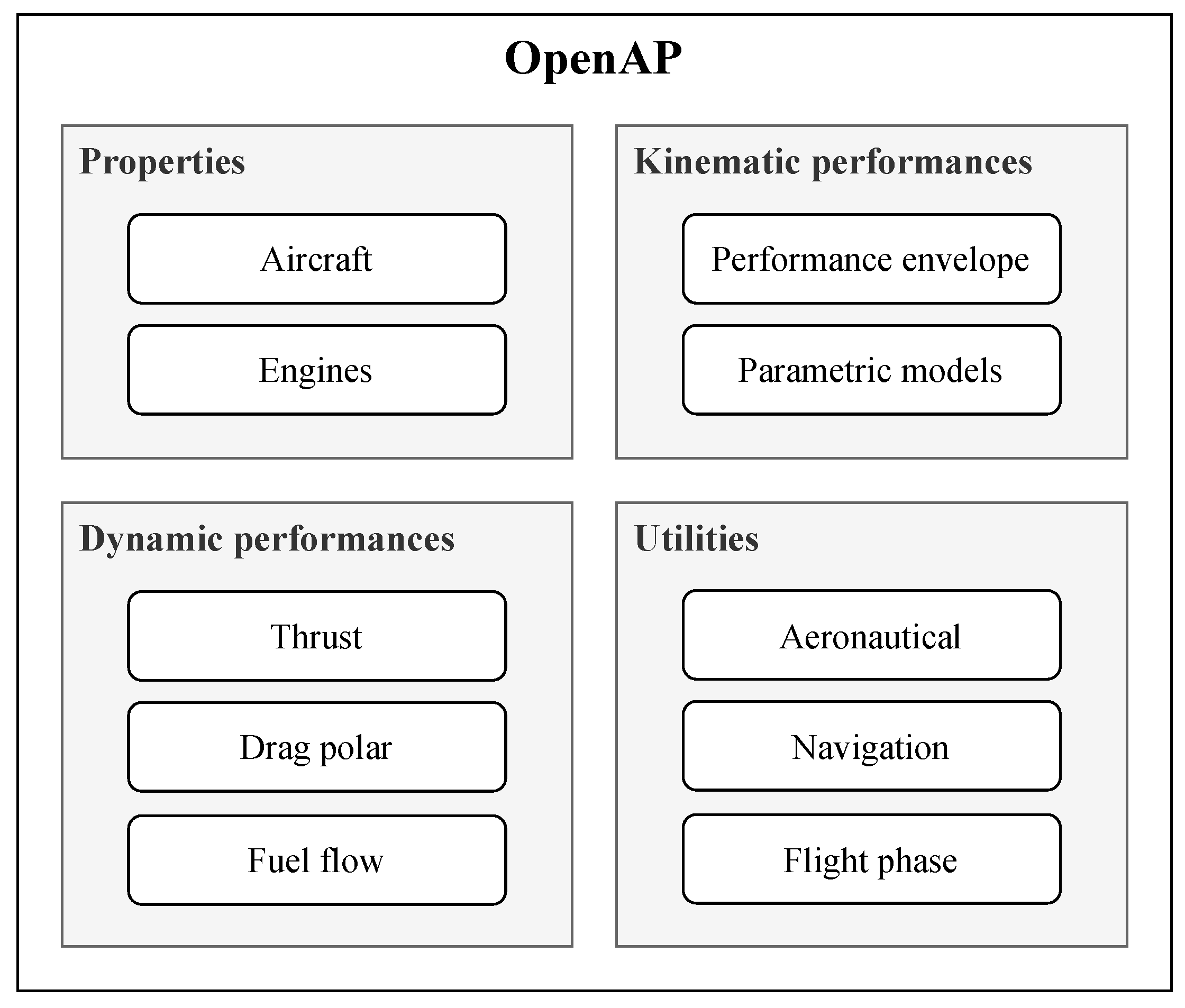
The OpenAP model consists of four main components, which are the aircraft properties, kinematic performances, dynamic performances, and utilities. In each main component, there can be multiple sub-components. Figure 1 shows the structure of OpenAP model at the current stage.

Figure 1. The structure of OpenAP.

In OpenAP, multiple formats exist to effectively store different types of data. The main file format is YAML format [16], which, according to its developer, is a human-friendly data serialization standard. It is primarily a key-value based document definition that can be easily interpolated by both humans and programming languages. For example, aircraft properties and drag polar models are presented using the YAML file format. YAML is effective for storing a key-value-like data structure but not efficient for larger tabular data. In these cases, the fixed width text files are used. They can be easily processed by computers while still maintaining readability for users. For example, the engine and kinematic performance databases are stored using fixed-width text files.

OpenAP aims to be a practical model with easy applicability. Hence, we have designed the toolkit alongside the model using one of the most common scientific programming languages—Python. The toolkit interacts with the model data and implements the equations for different calculations. It gives other high-level applications easy access to the OpenAP model. For example, one can obtain the aircraft configurations and parameters of a specific engine as shown in Appendix C.1.

3. Aircraft and Engine Properties

Following the previous example, the property module includes aircraft characteristics and engine configurations. It also provides performance data for a large number of engines. Currently, the most common aircraft types are included in this module. A list of supported aircraft is shown in Table A1 of the Appendix A. For each aircraft type, parameters such as dimensions, limits, nominal cruise conditions, and engine options are given. For example, the Airbus A320 aircraft parameters are shown in Appendix B.1.

The unit for dimensions and height in the configuration files is the meter, while the unit for weight is the kilogram. The aircraft data were gathered based on public data from aircraft manufacturers and the literature—for example, in [17,18].

Performance data on around 400 different engines are presented in the OpenAP engine databases (available at /openap/openap/data/engine of the OpenAP repository). Each engine has 11 parameters that are related to its performance. These parameters are indicated in Table 1. The first eight parameters are available for all engines. They are derived based on the ICAO aircraft engine emissions databank [19]. The last three parameters are only available for some engines; they were obtained from [20].

Table 1. Engine performance parameters

Parameter	Notation	Remarks
name	-	engine common identifier
manufacture	-	-
bpr	$\lambda$	bypass ratio
pr	-	pressure ratio
max_thrust	$T_0$	maximum static thrust, sea level (unit: N)
fuel_c3	$C_{\mathrm{ff}3}$	fuel flow coefficient, 3rd order term (unit: kg/s)
fuel_c2	$C_{\mathrm{ff}2}$	fuel flow coefficient, 2nd order term (unit: kg/s)
fuel_c1	$C_{\mathrm{ff}1}$	fuel flow coefficient, 1st order term (unit: kg/s)
cruise_thrust	$T_{\mathrm{cr}}$	thrust at the top of climb (unit: N)
cruise_mach	$M_{\mathrm{cr}}$	cruise Mach number for the thrust condition
cruise_alt	$h_{\mathrm{cr}}$	cruise Mach altitude for the thrust condition (unit: ft)

4. Kinematic Performance

The kinematic model studies the motion of the aircraft without considering the force acting on the aircraft. In OpenAP, the kinematic performance database is based on the results of a data-driven statistical model (WRAP) which was proposed in our previous study [15].

The WRAP model divides the flight into seven flight phases. It models different performance parameters at each flight phase accordingly. These performance indicators are acceleration, speed, vertical rate, altitude, and distance. Sorted by the flight phase, the parameters for kinematic performance are listed in Table 2.

Table 2. Performance parameter in OpenAP kinematic model.

Takeoff	${\mathit{V}}_{\mathbf{lof}}$ $d_{\mathrm{tof}}$ ${\overline{a}}_{\mathrm{tof}}$	liftoff speed takeoff distance mean takeoff acceleration	m/s km m/s${}^2$
Initial climb	$V_{\mathrm{cas},\mathrm{ic}}$ ${V_S}_{\mathrm{ic}}$	calibrated airspeed vertical rate	m/s m/s
Climb	$R_{\mathrm{top},\mathrm{cl}}$ $h_{\mathrm{cas},\mathrm{cl}}$ $V_{\mathrm{cas},\mathrm{cl}}$ ${V_S}_{\mathrm{cas},\mathrm{cl}}$ $h_{\mathrm{mach},\mathrm{cl}}$ $M_{\mathrm{cl}}$ ${V_S}_{\mathrm{mach},\mathrm{cl}}$ ${V_S}_{\mathrm{precas},\mathrm{cl}}$	range to the top of climb constant CAS crossover altitude constant CAS vertical rate during constant CAS climb constant Mach climb crossover altitude constant Mach number vertical rate at constant Mach climb vertical rate before constant CAS climb	km km m/s m/s km - m/s m/s
Cruise	$R_{\mathrm{cr}}$ $h_{\mathrm{init},\mathrm{cr}}$ $h_{\mathrm{cr}}$ $M_{\mathrm{cr}}$	cruise range initial cruise altitude cruise altitude cruise Mach number	km km km -
Descent	$R_{\mathrm{top},\mathrm{de}}$ $M_{\mathrm{de}}$ $h_{\mathrm{mach},\mathrm{de}}$ ${V_S}_{\mathrm{mach},\mathrm{de}}$ $V_{\mathrm{cas},\mathrm{de}}$ $h_{\mathrm{cas},\mathrm{de}}$ ${V_S}_{\mathrm{cas},\mathrm{de}}$ ${V_S}_{\mathrm{postcas},\mathrm{de}}$	range from the top of descent constant Mach number constant Mach descent crossover altitude vertical rate at constant Mach descent constant CAS constant CAS crossover altitude vertical rate at constant CAS descent vertical rate after constant CAS descent	km - km m/s m/s km m/s m/s
Final approach	$V_{\mathrm{cas},\mathrm{fa}}$ ${V_S}_{\mathrm{fa}}$ ${\angle }_{\mathrm{fa}}$	calibrated airspeed vertical rate path angle	m/s m/s deg
Landing	$V_{tcd}$ $d_{lnd}$ ${\overline{a}}_{lnd}$	touchdown speed braking distance mean braking deceleration	m/s km m/s${}^2$

By combining all the parameters, the kinematic module can describe the trajectory from takeoff until landing for the aircraft types as listed in Table A1.

The trajectory of the aircraft can be constructed using a set of ordinary differential equations. Under the International Standard Atmosphere (ISA) condition and without wind, the differential equations are expressed as:

$$\begin{array}{cc}\hfill \frac{\mathrm{d}x}{\mathrm{d}t}& =V\sin \psi \hfill \end{array}$$

(1)

$$\begin{array}{cc}\hfill \frac{\mathrm{d}y}{\mathrm{d}t}& =V\cos \psi \hfill \end{array}$$

(2)

$$\begin{array}{cc}\hfill \frac{\mathrm{d}h}{\mathrm{d}t}& =V_S\hfill \end{array}$$

(3)

$$\begin{array}{cc}\hfill \frac{\mathrm{d}V}{\mathrm{d}t}& =a\hfill \end{array}$$

(4)

where V represents the ground speed of the aircraft, which is the same as true airspeed without wind. It can be computed from either calibrated airspeed or Mach number depending on the flight phase.

The true airspeed can be computed from calibrated airspeed using the following equations:

$$\begin{array}{cc}\hfill V& =\sqrt{\frac{7p}{\rho }\left[{\left(1+\frac{q_c}{p}\right)}^{\frac{2}{7}}-1\right]}\hfill \end{array}$$

(5)

$$\begin{array}{cc}\hfill q_c& =p_0\left[{\left(1+\frac{{\rho }_0}{7p_0}{V}_{\mathrm{cas}}^2\right)}^{\frac{7}{2}}-1\right]\hfill \end{array}$$

(6)

where $q_c$ represents the impact pressure. In cases where the Mach number is given, the true airspeed can be calculated using temperature ($\tau$) and speed of sound (a) as:

$$V=a_{0}M\sqrt{\frac{\tau }{{\tau }_0}}$$

(7)

where $\rho$, p, and $\tau$ can be obtained from the ISA model if one knows the altitude of the aircraft. For cases other than ISA, deviations from ISA conditions, such as temperature, pressure, and wind, are considered to compute the actual ground speed. It is worth noting that in real operations, pressure, temperature, and wind can be derived based on aircraft Enhanced Mode S Surveillance (EHS) data and ADS-B data, which is described in detail in [21].

Each parameter from the WRAP kinematic model is provided with a default value, minimum value, maximum value, and parametric statistical model. The minimum and maximum values provide the boundaries of the parameter, while the parametric statistical model can be used to sample values from a given probability density function (normal, gamma, or beta). With the OpenAP toolkit, all kinematic performance parameters can be queried using the functions defined in Appendix C.2. Each of the functions returns the default, minimum, maximum, and parameters to construct the probability density function that reflects the performance indicator. The model default value refers to the most common value for each parameter. The detail on obtaining these parameters can be found in [15].

5. Dynamic Performance

To further extend OpenAP capabilities, the dynamic module is included. In addition to speed, vertical rate, and distance, the dynamic module deals with more performance parameters, specifically, the mass and forces. The main challenge of constructing a complete dynamic model is the lack of open data on aircraft mass, thrust, and drag models. OpenAP accomplishes the goal by using models from the literature and open flight data. Another important part of the dynamic module is to express the fuel consumption of different engines during operation. To achieve this, the ICAO aircraft engine emissions databank was used to construct the fuel flow model.

5.1. Aircraft Dynamic Model

Aircraft motion in OpenAP is defined using a four-degrees-of-freedom point-mass model, which describes the aircraft translations in three perpendicular axes, and the roll rotation. In this point-mass model, the forces are assumed to be applied at the aircraft’s center of gravity. The model can also be expressed with a set of ordinary differential equations. Assuming the ISA and zero wind, these equations can be written as:

$$\begin{array}{cc}\hfill \frac{\mathrm{d}x}{\mathrm{d}t}& =V\sin \psi \cos \gamma \hfill \end{array}$$

(8)

$$\begin{array}{cc}\hfill \frac{\mathrm{d}y}{\mathrm{d}t}& =V\cos \psi \cos \gamma \hfill \end{array}$$

(9)

$$\begin{array}{cc}\hfill \frac{\mathrm{d}h}{\mathrm{d}t}& =V\sin \gamma \hfill \end{array}$$

(10)

$$\begin{array}{cc}\hfill \frac{\mathrm{d}\psi }{\mathrm{d}t}& =\frac{g\tan \varphi }{V\cos \gamma }\hfill \end{array}$$

(11)

$$\begin{array}{cc}\hfill \frac{\mathrm{d}V}{\mathrm{d}t}& =\frac{T-D}{m}-g\sin \gamma \hfill \end{array}$$

(12)

$$\begin{array}{cc}\hfill \frac{\mathrm{d}m}{\mathrm{d}t}& =f_{\mathrm{fuel}}(T,h)\hfill \end{array}$$

(13)

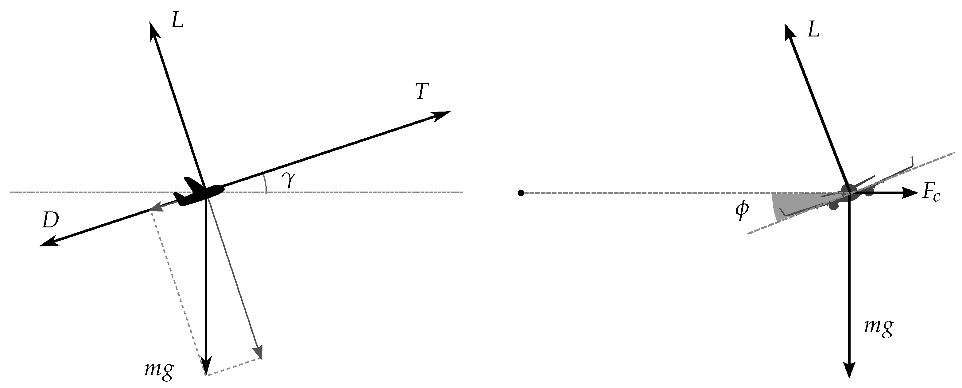
The dynamic components introduced in these differential equations are mass, thrust, drag, and fuel flow. In Figure 2, forces acting on the aircraft in the dynamic model are illustrated.

Figure 2. Forces acting on the aircraft in the point-mass dynamic performance model.

On the left-hand side of the figure, different forces are viewed from the side view. The right-hand side of the figure shows the forces during the banking from the front view. $F_c$ refers to the centrifugal force, which is not explicitly expressed in the model.

The net thrust is expressed as the product throttle setting (${\delta }_T$) and the maximum thrust. Based on an empirical model proposed by [22], the maximum thrust of the aircraft ($f_{\mathrm{thr}}$) is expressed as a function that is dependent on the aircraft altitude, speed, and vertical rate:

$$\begin{array}{cc}\hfill T& ={\delta }_T{f}_{\mathrm{thr}}(h,V,V_S)\hfill \end{array}$$

(14)

The drag force of the aircraft in Equation (12) can be calculated knowing the dynamic pressure (q), the wing surface (S), and the drag coefficient ($C_D$):

$$\begin{array}{cc}\hfill D& =C_{D}qS\hfill \end{array}$$

(15)

$$\begin{array}{cc}\hfill q& =\frac{1}{2}\rho V^2\hfill \end{array}$$

(16)

The fuel flow model used in Equation (13) is a function that is dependent on the net thrust of the aircraft’s engines. It is constructed using the fuel flow coefficients proposed in the engine performance database that is shown in Table 1. The details of the thrust, drag, and fuel flow models are explained in the rest of this section.

5.2. Thrust

The thrust model included in OpenAP can calculate maximum takeoff thrust and maximum thrust separately during the flight. The key parameters that determine the maximum thrust of the turbofan engine are the maximum static thrust at sea level ($T_0$), the bypass ratio ($\lambda$), and the rated engine thrust at cruise. Most numerical coefficients in the thrust equations are obtained empirically from available performance data from multiple engines according to [22].

5.2.1. Takeoff Thrust

Considering the altitude of the runway, the takeoff thrust of an engine is modeled as:

$$\frac{T}{T_0}=A-\frac{0.377(1+\lambda )}{\sqrt{(1+0.82\lambda )G_0}}ZM+(0.23+0.19\sqrt{\lambda })X{M}^2$$

(17)

where the coefficient of the parameter is calculated as follows:

$$\begin{array}{cc}\hfill G_0& =0.0606\lambda +0.6337\hfill \end{array}$$

(18)

$$\begin{array}{cc}\hfill A& =-0.4327{\left(\frac{p}{p_0}\right)}^2+1.3855\frac{p}{p_0}+0.0472\hfill \end{array}$$

(19)

$$\begin{array}{cc}\hfill Z& =0.9106{\left(\frac{p}{p_0}\right)}^3-1.7736{\left(\frac{p}{p_0}\right)}^2+1.8697\frac{p}{p_0}\hfill \end{array}$$

(20)

$$\begin{array}{cc}\hfill X& =0.1377{\left(\frac{p}{p_0}\right)}^3-0.4374{\left(\frac{p}{p_0}\right)}^2+1.3003\frac{p}{p_0}\hfill \end{array}$$

(21)

5.2.2. Climb and Cruise Thrust

The climb is divided into three segments to compute the thrust. The segments are 0–10 k ft, 10–30 k ft, and 30–40 k ft. An additional key parameter is the engine thrust during the cruise at 30 k ft according to [22]. In OpenAP, a small modification is made so that the cruise altitude is not fixed at 30 k ft. Instead, the cruise altitude from the aircraft and engine property module is used.

(i)

For the en-route segment from 30 k ft to 40 k ft, the thrust ratio is modeled as follows:

$$\frac{T}{T_{\mathrm{cr}}}=c_1\ln \left(\frac{p}{p_{\mathrm{cr}}}\right)+c_2$$

(22)

where $c_1$ and $c_2$ are calculated as:

$$\begin{array}{cc}\hfill c_1& =-0.4204\left(\frac{M}{M_{\mathrm{cr}}}\right)+1.0824\hfill \\ \hfill c_2& ={\left(\frac{M}{M_{\mathrm{cr}}}\right)}^{-0.11}\hfill \end{array}$$

(23)

(ii)

For the segment from 10 k ft to 30 k ft, the thrust is derived similarly, with the exception that the reference calibrated airspeed is used instead of Mach number. The thrust can be approximated as:

$$\frac{T}{T_{\mathrm{cr}}}=c_3{\left(\frac{p}{p_{\mathrm{cr}}}\right)}^{c_4}$$

(24)

where the coefficients $c_3$ and $c_4$ are calculated as follows:

$$\begin{array}{cc}\hfill c_3& ={\left(\frac{V_{cas}}{V_{cas,cr}}\right)}^{-0.1}\hfill \\ \hfill c_4& =-0.335\left(\frac{V_{cas}}{V_{cas,cr}}\right)+c_5\hfill \end{array}$$

(25)

In order to find the value of $c_5$, a look-up table is used in [22]. To simplify the computation, a linear approximation for $c_5$ is adopted in OpenAP as follows:

$$c_5=2.667\times {10}^{-5}{V}_S+0.8633$$

(26)

where the unit of $V_S$ is in m/s.

(iii)

For the climbing segment from takeoff up to 10 k ft, a linear model is used to approximate the thrust ratio, with respect to the thrust ratio at 30 k ft. The relationship is as follows:

$$\frac{T}{T_{\mathrm{cr}}}=c_6\left(\frac{p}{p_{\mathrm{cr}}}\right)+\left[\frac{T_{10}}{T_{\mathrm{cr}}}-c_6\left(\frac{p_{10}}{p_{\mathrm{cr}}}\right)\right]$$

(27)

where $T_{10}$ is the thrust at 10k ft. It can be computed by first using Equation (24). Coefficient $c_6$ is introduced to incorporate the variations in speeds and vertical rates. In [22], a look-up table is also used to find the value of $c_6$. In OpenAP, a bi-variate polynomial function is constructed to approximate this coefficient instead:

$$\begin{array}{cc}\hfill c_6=& -1.2043\times {10}^{-1}\left(\frac{V_{\mathrm{cas}}}{V_{\mathrm{cas},\mathrm{cr}}}\right)-8.8889\times {10}^{-9}{V_S}^2\hfill \\ & +2.4444\times {10}^{-5}{V}_S+4.7379\times {10}^{-1}\hfill \end{array}$$

(28)

where the units of $V_{\mathrm{cas}}$ and $V_S$ are both in m/s.

5.2.3. Reference Cruise Thrust

One of the parameters used in the thrust model is the rated thrust at cruise altitude ($T_{\mathrm{cr}}$). However, this information is not always published by aircraft or engine manufacturers. Available engine reference data are included in the engine performance (shown in Table 1). When $T_{\mathrm{cr}}$ is not available, we rely on the empirical model proposed in [20], where the cruise thrust model is constructed for the maximum static thrust as:

$$T_{\mathrm{cr}}=0.2T_0+890$$

(29)

where the units of $T_{\mathrm{cr}}$ and $T_0$ are both in N.

Using the OpenAP toolkit, the maximum thrust of the aircraft during the flight can be conveniently computed following the example in Appendix C.3.

5.3. Drag

To compute the drag of aircraft, we first need to determine the drag coefficient. The drag coefficient is dependent on the drag polar and the lift. In our previous study [23,24], drag polar models for common aircraft types were estimated (data available at /openap/openap/data/dragpolar of the OpenAP repository).

When an aircraft is airborne, the equations to calculate the drag coefficient are expressed as follows:

$$\begin{array}{cc}\hfill C_D& =C_{D0}+k{C}_L^2\hfill \end{array}$$

(30)

$$\begin{array}{cc}\hfill C_L& =\frac{L}{qS}=\frac{mg\cos \gamma }{qS}\hfill \end{array}$$

(31)

where the zero-lift drag coefficient ($C_{D0}$) and lift-induced drag coefficient (k) are provided by OpenAP. In the OpenAP toolkit, these parameters at different flight phases are presented. An example of the drag polar model is shown in Appendix B.2.

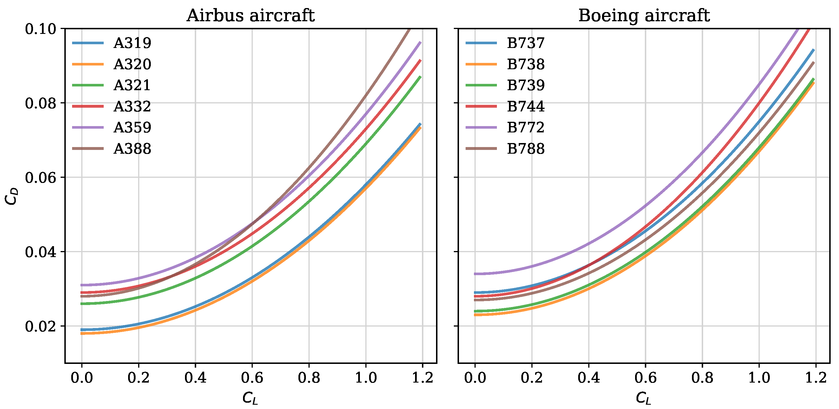
Currently, the OpenAP model contains the drag polars for around 20 of the most common aircraft types. For illustration purposes, the drag polars for several common Airbus and Boeing aircraft types are visualized in Figure 3.

Figure 3. Drag polar estimated for common Airbus and Boeing aircraft under clean configurations at low Mach number.

5.4. Flaps

In addition to the drag polar of clean configuration, the OpenAP toolkit provides the model to compute the increase in drag coefficient under different flaps configurations. Using an empirical model ([25], p.109), this increase in drag coefficient due to flap deflection can be computed as:

$$\Delta C_{D,f}={\lambda }_f{\left(\frac{c_f}{c}\right)}^{1.38}\left(\frac{S_f}{S}\right){\sin }^2{\delta }_f$$

(32)

where $c_f/c$ and $S_f/S$ are flap to wing chord ratio and flap to wing surface ratio respectively. ${\delta }_f$ is the flap deflection angle. When exact $c_f/c$ and $S_f/S$ are not available, they are both assumed to be 0.15, which is an empirical approximation based on existing aircraft data. ${\lambda }_f$ is dependent on the type of flaps. According to [25], ${\lambda }_f$ is set to be 1.7 for plain and split flaps and 0.9 for slotted flaps.

Changes in lift-induced drag coefficient due to flaps can also be modeled. The deflection of flaps affects the Oswald efficiency factor (e). Based on data from several existing aircraft, a linear relationship was found by [26]. The model to calculate such an increase in e due to flaps (denoted as $\Delta e_f$) is:

$$\begin{array}{ccc}\Delta e_f=0.0046{\delta }_f\hfill & & (\mathrm{for}\mathrm{rear}-\mathrm{mounted}\mathrm{engines})\hfill \\ \Delta e_f=0.0026{\delta }_f\hfill & & (\mathrm{for}\mathrm{wing}-\mathrm{mounted}\mathrm{engines})\hfill \end{array}$$

(33)

5.5. Compressibility

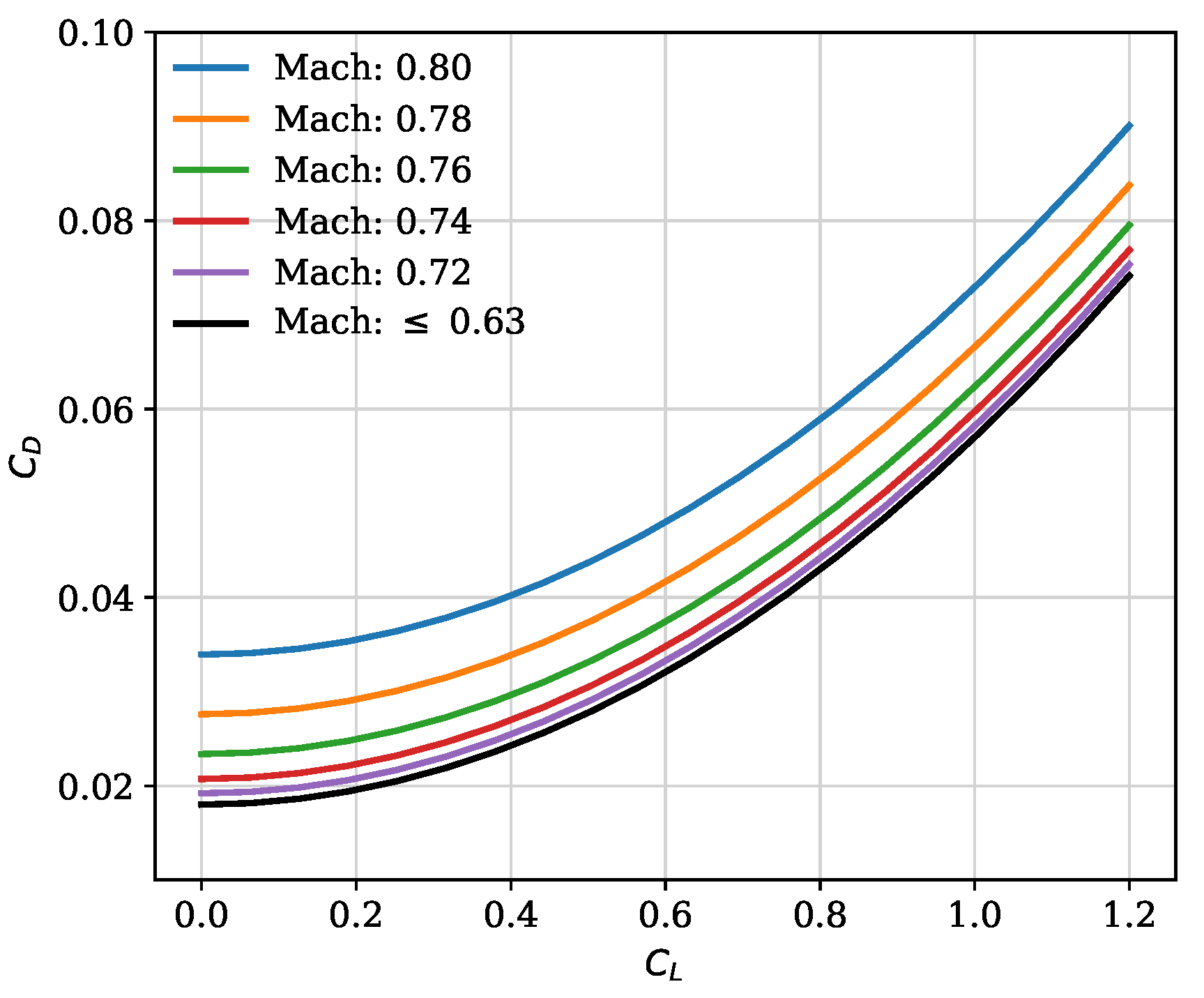
When an aircraft flies at a higher speed than critical Mach number, the compressibility effect should not be ignored. In OpenAP, the increase of drag coefficient due to wave drag $\Delta C_{D,w}$ is modeled as [27]:

$$\Delta C_{D,w}=\left\{\begin{array}{cc}0\hfill & M\le M_{\mathrm{crit}}\hfill \\ 20{(M-M_{\mathrm{crit}})}^4\hfill & M>M_{\mathrm{crit}}\hfill \end{array}\right.$$

(34)

where $M_{\mathrm{crit}}$ is the critical Mach number which is given by OpenAP. In Figure 4, the compressibility effect on drag polar for one aircraft is shown.

Figure 4. Changes of drag polar due to compressibility (A320).

5.6. Landing Gear

The landing gear adds a significant amount of drag to an aircraft when it is extended. It is retracted as soon as the aircraft becomes airborne and only extended shortly before landing. There are limited studies that quantify the drag coefficients of aircraft landing gear. In this paper, we adopted the model proposed by [28] to calculate the increased drag coefficient created by landing gear:

$$\Delta C_{D,g}=\frac{W}{S}{K}_{\mathrm{uc}}{m}_{\max }^{-0.215}$$

(35)

where $W/S$ is the wing loading, $m_{\max }$ refers to the maximum mass of an airplane, and $K_{\mathrm{uc}}$ is a factor that relates to the flap deflection angle. In principle, the value of $K_{\mathrm{uc}}$ is lower when more flap deflection is applied. This is because the flow velocity along the bottom of the wing decreases when flaps are deployed, which leads to a lower drag on the landing gear. For simplification, it is taken as $3.16\times {10}^{-5}$ in this paper based on the data provided by [28].

5.7. Final Drag Polar Model

In summary, combining all the components discussed in this section, the zero-lift drag coefficient is calculated as:

$$C_{D0}=C_{D0,clean}+\Delta C_{D,f}+\Delta C_{D,g}+\Delta C_{D,w}$$

(36)

Additionally, the lift-induced drag coefficient is calculated as:

$$k=\frac{1}{1/k_{clean}+\pi A\Delta e_f}$$

(37)

Knowing the aircraft mass, airspeed, altitude, and flight path angle, the drag of the aircraft can be computed following the example in Appendix C.4.

5.8. Fuel Flow

The engine fuel flow model was constructed based on the public data obtained from the ICAO aircraft engine emissions databank [19]. Fuel flow indicators for most turbofan engines are included in this database. It defines fuel flow under four different conditions, which are takeoff, climb-out, approach, and idle. The power settings of the engine are defined at 100%, 85%, 30%, and 7% of engine maximum power respectively. Under the static sea-level testing condition, engine fuel flow data were obtained and published.

In order to create a model that can compute actual fuel consumption under different thrust, these four data points are fitted with a 3rd-degree polynomial model. The coefficients for the polynomial function are defined as $C_{\mathrm{ff}}3$, $C_{\mathrm{ff}}2$, and $C_{\mathrm{ff}}1$ (as shown in Table 1), with the unit of kg/s. The fuel flow profile defines the relationship between fuel flow and percentage of the maximum static thrust. Denoting $f_{\mathrm{fuel},\mathrm{SL}}$ as the function representing fuel flow (kg/s) at sea level, the dynamic fuel flow model can be computed knowing the net thrust:

$$f_{\mathrm{fuel},\mathrm{SL}}\left(T\right)=C_{\mathrm{ff}3}{\left(\frac{T}{T_0}\right)}^3+C_{\mathrm{ff}2}{\left(\frac{T}{T_0}\right)}^2+C_{\mathrm{ff}1}\frac{T}{T_0}$$

(38)

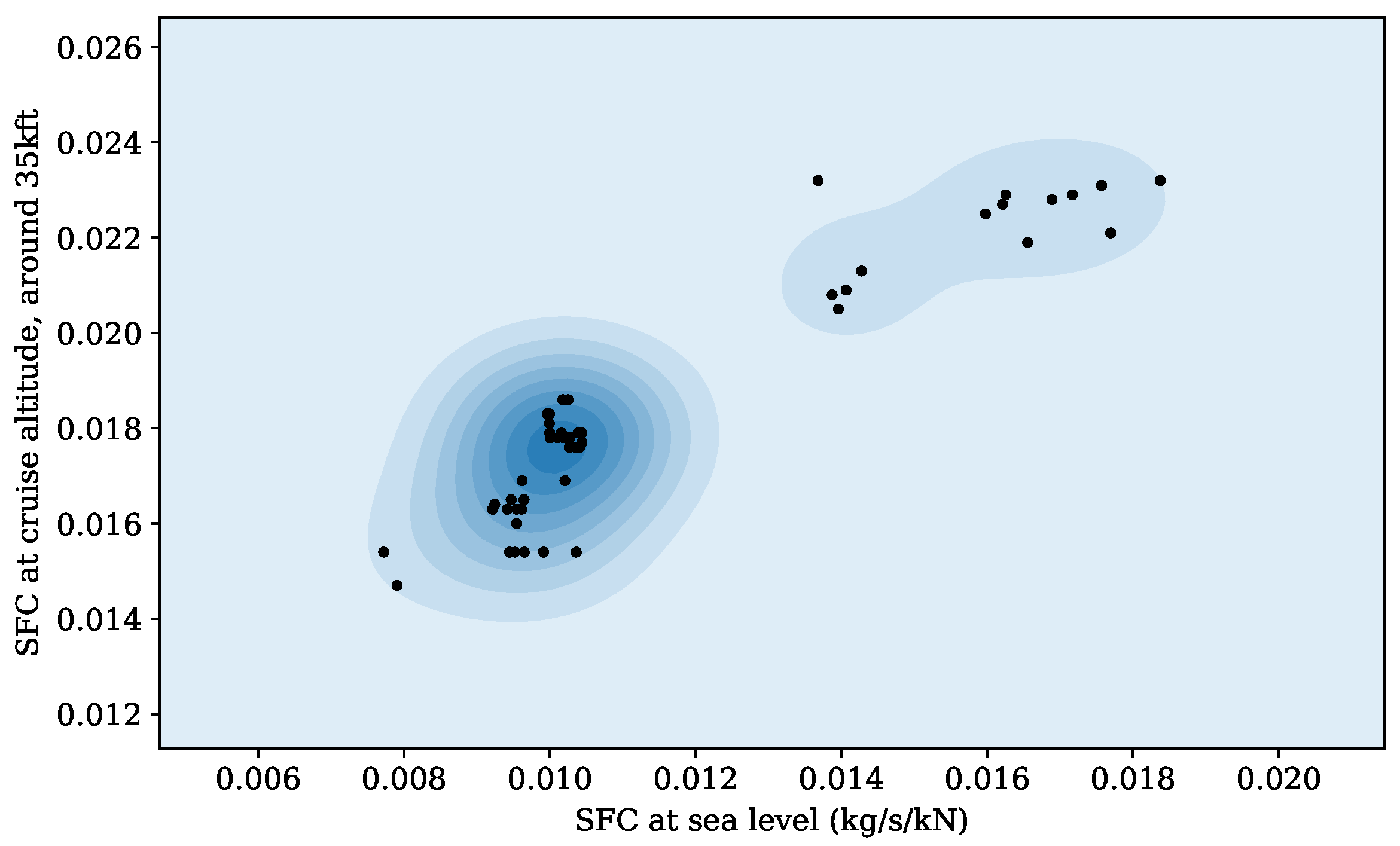
where all the coefficients and maximum static thrust $T_0$ of each engine are given in the engine database of OpenAP. For the same amount of thrust, fuel flow increases with altitude. This difference can be seen by the thrust’s specific fuel consumption (SFC) at sea-level and cruise conditions. In Figure 5, the differences for multiple engines are shown.

Figure 5. Differences in specific fuel consumption at sea level and cruise altitude.

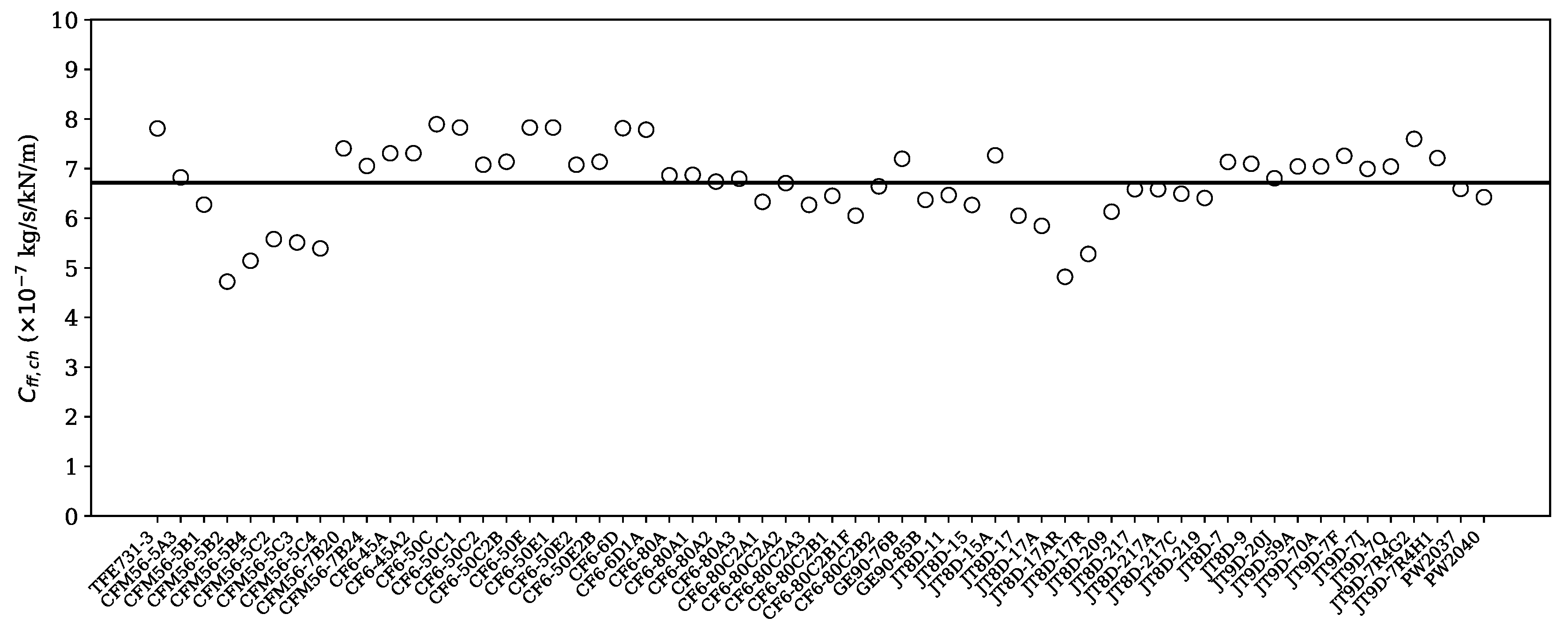
Based on the limited data on SFC at sea level and cruise altitude, we propose a simplified linear correction factor ($C_{\mathrm{ff},\mathrm{ch}}$) that takes into consideration the altitude effect. When SFC is available at the cruise altitude, the correction factor is calculated as:

$$\begin{array}{cc}\hfill C_{\mathrm{ff},\mathrm{ch}}& =\frac{{\mathrm{SFC}}_{\mathrm{CR}}-{\mathrm{SFC}}_{\mathrm{SL}}}{h_{\mathrm{CR}}}\hfill \\ & =\frac{{\mathrm{SFC}}_{\mathrm{CR}}-f_{\mathrm{fuel},\mathrm{SL}}\left(T_0\right)/T_0}{h_{\mathrm{CR}}}\left(\mathrm{unit}\text{:}\frac{kg}{s\times kN\times m}\right)\hfill \end{array}$$

(39)

where the $h_{\mathrm{CR}}$ is the cruise altitude for the corresponding SFC.

Figure 6 illustrates the coefficient for engines with available ${\mathrm{SFC}}_{\mathrm{CR}}$. The mean value was found to be around $6.7\times {10}^{-7}$, which is used as a default value for engines where ${\mathrm{SFC}}_{\mathrm{CR}}$ is not available.

Figure 6. Difference in specific fuel consumption at sea level and cruise altitude.

Combining the fuel flow at sea level and the fuel flow with altitude correction, the dynamic fuel flow can be computed. The final fuel flow model is expressed as:

$$\begin{array}{cc}\hfill f_{\mathrm{fuel}}(T,h)& =f_{\mathrm{fuel},\mathrm{SL}}\left(T\right)+C_{\mathrm{ff},\mathrm{ch}}\times T\times h\hfill \\ & =C_{\mathrm{ff}3}{\left(\frac{T}{T_0}\right)}^3+C_{\mathrm{ff}2}{\left(\frac{T}{T_0}\right)}^2+C_{\mathrm{ff}1}\frac{T}{T_0}+C_{\mathrm{ff},\mathrm{ch}}\times T\times h\hfill \end{array}$$

(40)

In OpenAP, the fuel flow can be computed under three conditions: (1) with a known net thrust of all engines; (2) during the takeoff with a known thrust setting and an unknown aircraft mass; (3) during the flight, knowing the mass, speed, altitude, and flight path angle. In general, when net thrust is not known, it can be calculated based on the dynamic model (Equation (12)). Examples of calculating the fuel flow are given in Appendix C.5.

6. Other Databases and Utility Libraries

Besides the core components explained in the earlier sections, OpenAP also provides several utility libraries to facilitate calculations related to aircraft performance.

6.1. Flight Phase

Based on our earlier research [29], the flight phase library enables the easy use of the fuzzy logic flight phase identification algorithm. Providing the trajectory (with time, altitude, speed, and vertical rate), one can obtain corresponding flight phases for the entire trajectory. The flight data are labeled with the ground, climb, cruise, descent, and leveling phases.

Functions in the flight phase library also enable the extraction of specific flight segments among all available flight phases, which are takeoff, initial climb, climb, cruise, descent, final approach, and landing. Examples are shown in Appendix C.6.

6.2. Aeronautical Calculations

Derived from the open-source BlueSky simulator, the aeronautical library provides common calculations related to aircraft performance. For example, this library provides the functions to compute distance and bearing. It is also able to calculate the standard atmospheric conditions at different flight levels. In addition, speed conversions among calibrated airspeed (CAS), true airspeed (TAS), and Mach number (e.g., Equations (5) and (7)) are easily made with this library.

6.3. Navigation Database

The navigation database provides information on airport and navigation data (available at /openap/openap/data/nav of the OpenAP repository). The data in the navigation database are based on the open data published by X-Plane [30]. The navigation library is designed to give easy access to these datasets. For example, the airport location can be queried using its ICAO code. One can also use this library to get the closest airport or fixes of a specific location. Examples are shown in Appendix C.7.

7. Analysis of OpenAP

In this section, analyses are conducted to examine the OpenAP model. Firstly, maximum thrust profiles computed using OpenAP and BADA 3 are compared. Then, using a test flight from the TU Delft Cessna Citation aircraft, both thrust and fuel flow from OpenAP are compared to the onboard data. In addition, the same values are computed from the BADA model to serve as a comparison.

7.1. Trajectory Generation

The OpenAP toolkit comes with a kinematic trajectory generator that can be used to quickly generate a large number of flight trajectories. The generator creates trajectories based on the WRAP kinematic model (Equations (1)–(4)). Users can specify the initial conditions and time step, or leave them to the program. When left to the program, the performance parameter values can be requested as the default values or random values to be drawn from the corresponding probability density function. When a complete trajectory needs to be generated, speed profiles of the climb, cruise, and descent phases are coupled based on the cruise altitude and Mach number. An example of this trajectory generation method is explained in Appendix C.8.

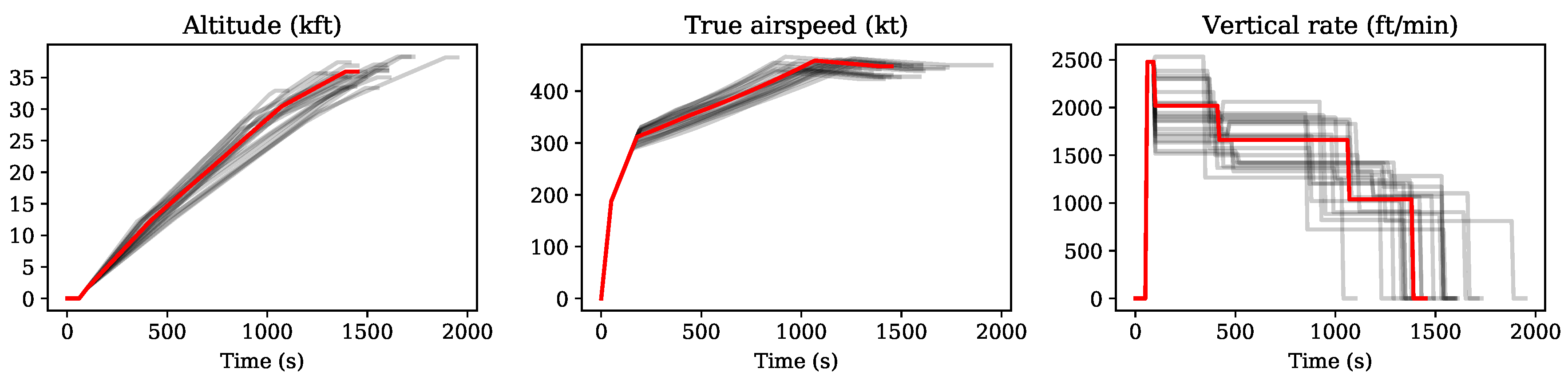
In the following use case, several simple flight trajectories are generated. In Figure 7 and Figure 8, the vertical profiles of a number of generated climbing and descent trajectories are shown. The default (most common) profile is indicated in red, while a set of randomly generated profiles is shown in gray.

Figure 7. Generated climbing trajectory (Airbus A320).

Figure 8. Generated descent trajectory (Airbus A320).

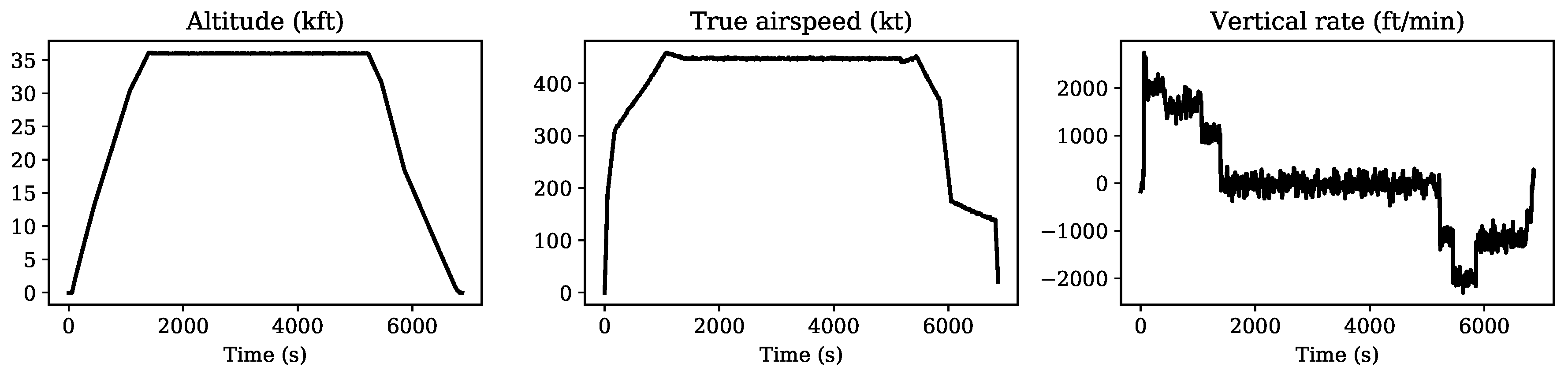
Based on the noise characteristics from ADS-B, the trajectory generator also allows simulated observation noise to be added to generated trajectories. In Figure 9, one such example is shown as a complete trajectory with Gaussian noise added.

Figure 9. Generated complete trajectory with noise added (Airbus A320).

7.2. Comparison with BADA

7.2.1. Thrust Model

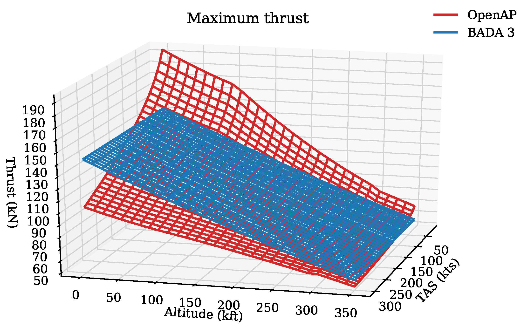
To demonstrate the difference between OpenAP and BADA, we computed the maximum thrust of an aircraft (Airbus A320 with V2500-A1 engines) under different flight conditions. The results are shown in Figure 10. The maximum thrust was computed using different combinations of altitude and speed. OpenAP and BADA results are illustrated in red and blue respectively.

Figure 10. A320 maximum thrust (V2500-A1 engine).

A large difference is visible when the aircraft is at low altitude. The difference between OpenAP and BADA becomes smaller when the aircraft is flying at a higher altitude. One of the major reasons for the difference is that BADA 3 does not model thrust dynamic due to the change of airspeed. In contrast, OpenAP shows a clear nonlinear relationship between aircraft speed and thrust. The performance is more realistic for a lower altitude at a lower speed.

7.2.2. Drag Polar

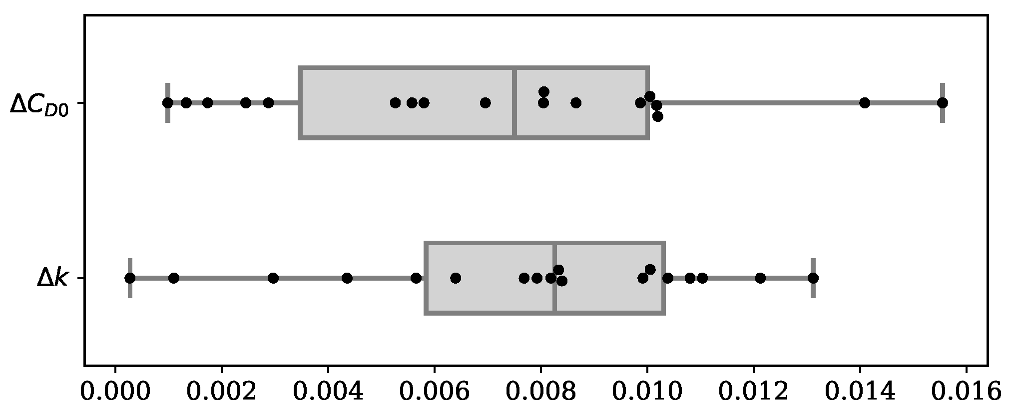
Due to the restrictions associated with the BADA license, exposure of specific BADA coefficients is not permitted. Instead of showing the exact difference between BADA and our model for each aircraft type, the overall statistics for all available aircraft are shown in Figure 11. The mean absolute differences for $C_{D0}$ and k were both found to be around 0.007.

Figure 11. Absolute difference of drag polar between BADA (3.12) and the model derived in this paper under clean configuration.

This gives a good indication of what the level of difference in the outcome of this study is, compared to well-established performance models. However, we should be cautious when interpreting this difference as the estimation accuracy. Since neither the method nor the data used for constructing BADA drag polar are published, it is hard to identify the uncertainties in the BADA model. Thus, the difference between the two models should not be directly used to quantify the accuracy of our model.

7.2.3. Fuel Flow Model

The main difference between OpenAP and BADA fuel flow models is the input parameters. The inputs for BADA fuel flow calculation are thrust and speed, while the inputs for OpenAP fuel flow calculation are thrust and altitude.

We can visually compare the inputs and outputs of both fuel flow models in Figure 12, which shows the different variability of the two fuel flow models regarding different input parameters.

Figure 12. A320 maximum thrust (V2500-A1 engine).

It can be seen that the performances of both the fuel flow model are similar at a lower thrust (for example, during the cruise). However, while the aircraft is flying with a higher thrust (for example, during the climb), the OpenAP fuel flow model is corrected concerning the altitude of the aircraft. It is also worth emphasizing that the inputs for both models are different. Thus, a better way to evaluate fuel flow estimations has to be based on real flight trajectories, which is shown in the following section.

7.3. Analysis Based on Flight FMS Data

To further evaluate the thrust and fuel flow models, we used a real flight to examine the performance of OpenAP. The flight data were gathered from the TU Delft Cessna Citation II flight data recorder. The flight data contained states such as position, altitude, speed, vertical rate, acceleration, and fuel flow, and the takeoff mass of the aircraft.

Based on the onboard data, we could reconstruct the true net thrust of the engine during the flight based on drag and acceleration. This was to be used as a reference when examining the thrust model. In Figure 13, the maximum thrust computed from OpenAP and BADA are shown alongside the net thrust computed from flight data.

Figure 13. Maximum thrust profile.

The flight recorder data also include the fan rotation speed (N1), which is expressed as a percentage of the maximum rotation speed. By combining the N1 value and the maximum thrust computed from OpenAP, we were able to derive the estimated net thrust during the flight. The same method was also applied to the BADA model to serve as a comparison. In Figure 14, the estimated net thrusts are shown against the true net thrust. The distribution of estimation error based on BADA and OpenAP is also shown in this figure.

Figure 14. Estimated net thrust based on maximum thrust profile and N1 settings.

It is noticeable that during the climb, the open thrust model can approximate the thrust with the same level accuracy or better than BADA. During the cruise, a relatively large difference existed for both models. It is important to note that this large difference could be due to the nonlinear relationship between the fan rotation speed and the actual throttle setting. It is also worth noting the difference between this practice flight and a normal passenger flight. Firstly, the aircraft was cruising at a lower altitude (around 10,000 ft) instead of the optimal altitude (commonly above 30,000 ft). Secondly, the flight procedure was designed to test the limits of flight performance. Thus, drastic changes in speed and altitude existed during the flight. These factors would contribute to the difference between true thrust and estimated thrust using either OpenAP or BADA. Nonetheless, we can see similar estimation results emerge using OpenAP and BADA.

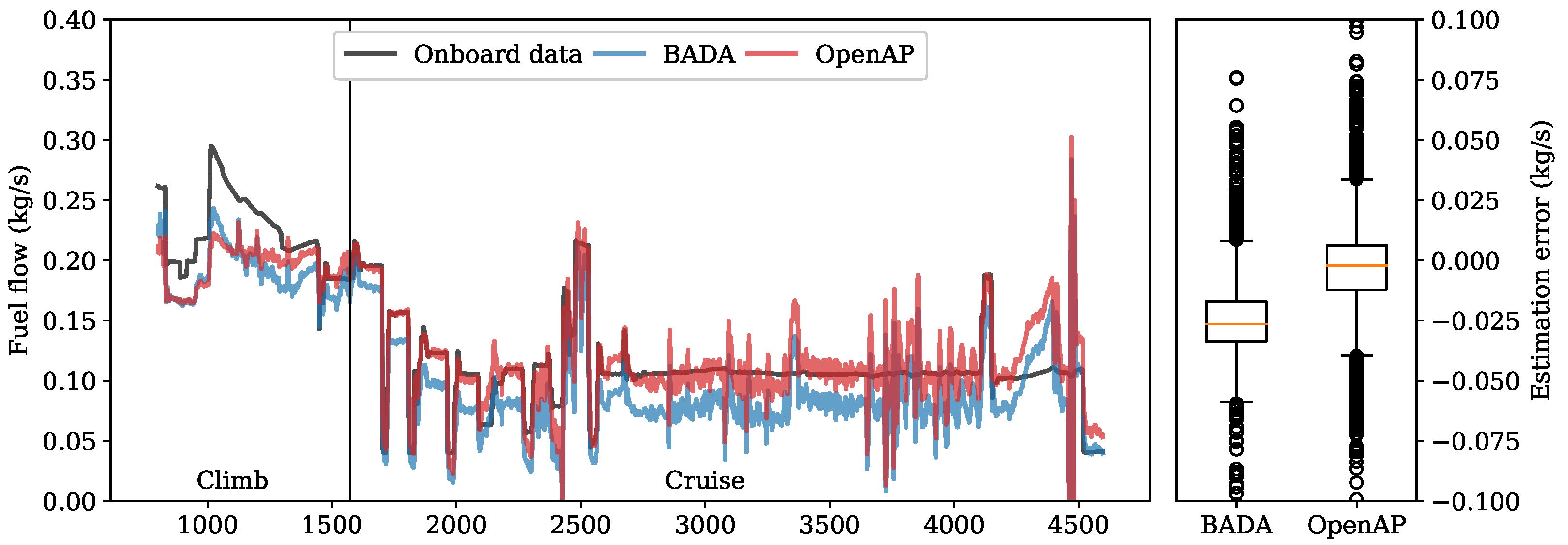
Using the recorded engine fuel flow data, the fuel flow model was evaluated. In Figure 15, the fuel flow is shown based on the the net thrust calculated based on onboard data. Results from OpenAP and BADA are illustrated alongside the actual fuel flow. The estimation error distributions of fuel flow using BADA and OpenAP are also shown.

Figure 15. Estimated fuel flow based on the net thrust.

Overall, OpenAP displays slightly better accuracy than BADA. It is also noticeable that the difference is higher when thrust is higher (during the climb). This can be seen as a reflection of the result that has been found in Figure 12.

8. Discussions

The OpenAP model and its associated toolkit are still under development. In this section, we address the limitations and plans for this aircraft performance model.

8.1. Limitations

As mentioned in the earlier sections, the thrust model included in OpenAP is based on the studies of [20,22], where only turbofan engines are modeled. Hence, OpenAP does not yet cover aircraft that are equipped with other engine types.

The thrust and fuel models used in OpenAP are based on external sources. Hence, the uncertainty in these third-party models and data affects the accuracy of the OpenAP model. Limited access to accurate flight data from a wider range of aircraft types also limits the validation of OpenAP.

As we are relying on a Bayesian estimation method, this creates uncertainty in the drag polar values described in this paper. There is also a certain level of uncertainty inherited from the thrust models and data, which is explained in [23].

Currently, only the most common civil aircraft types are covered in OpenAP. This is due to the availability of flight data. Though the aircraft diversity may be a limiting factor for some applications, the data-driven approach used to construct OpenAP allows more aircraft to be included with the growing volume of flight data in the future.

8.2. Future Development

The current research plan for OpenAP focuses on enhancing the models and providing more functionalities that can be beneficial for air transport research. Our current research efforts include:

• OpenAP Emission: Research is being conducted to incorporate an open emission model for emission and climate-related air transport studies.
• OpenAP Optimization: Based on the dynamic model, a trajectory optimization model shall be developed. This will further enhance the trajectory generation capability of OpenAP, extending from kinematic models to dynamic models.
• WRAP model: As more ADS-B data is collected, we plan to update the WRAP kinematic model every few years to include new aircraft types, as well as to improve models for less common aircraft types.

8.3. Sharing and Community Contributions

OpenAP model data and source code for the toolkit are published under the GNU GPL v3 license. This allows anyone to freely use (including commercial and private use), distribute, and change the content. The advantage of having such an open license is to allow easy access and encourage contributions from the air traffic management research community. The source code is published on GitHub, where anyone can take part in the future development of the model.

Part of OpenAP is derived from flight data based on our previous studies, for example, the drag polar and kinematic models. However, we welcome more accurate information to be submitted, as long as the data can be open and have been obtained from legitimate sources.

Currently, there are a limited number of flight test data included in the OpenAP repository as part of the open flight datasets. They are from the TU Delft Cessna Citation II aircraft. We welcome the input of flight test data from other aircraft types. The flight identifier can be anonymized. However, it would be ideal to maintain aircraft and engine types, airspeed, aircraft mass, and fuel flow information in the flight data.

9. Conclusions

In this paper, we explain the details of a new open aircraft performance model, OpenAP. The OpenAP model, which is the combined outcome of several of our previous studies, is aimed at providing the air traffic management research community an open alternative to current closed-source aircraft performance models. Accompanied by an off-the-shelf user library written in the Python programming language, the performance model consists of four major components, which are the aircraft and engine properties, kinematic performance, dynamic performance, and utility libraries.

The characteristics of 27 common aircraft and 400 turbofan engines have been included in the OpenAP properties library. The aircraft database provides basic information on aircraft dimensions, limits, and engine configurations. The engine database provides information such as maximum thrust, bypass ratio, cruise performance, and fuel flow coefficients for each engine type. The kinematic performance is produced by our previous data-driven model (WRAP). It describes parameters that are related to speed, vertical rate, distance, and height in seven distinct flight phases. The OpenAP toolkit enables easy access to these parameters. The dynamic performance module provides models that describe engine maximum thrust, fuel consumption, and drag polar. It allows OpenAP to be used independently for studies that require flight dynamics.

To provide more options for future air traffic management studies, future research on extending OpenAP will be focused on aircraft emission models and noise models. We also plan to include the trajectory optimization and prediction functionalities in the OpenAP toolkit. To promote open science and collaborations, all OpenAP model data and the toolkit source code are published on GitHub under the GNU GPL license, where future contributions and requests are welcomed.

Appendix B.1. Aircraft Property Data Structure

Data location: /openap/openap/data/aircraft/a320.yml

Appendix B.2. Drag Polar Data Structure

Data location: /openap/openap/data/dragpolar/a320.yml:

Appendix C.1. Access OpenAP Aircraft and Engines

Appendix C.2. Access WRAP Parameters

Appendix C.3. Calculate Aircraft Thrust

where the inputs of the function are true airspeed (in knots), altitude (in feet), and rate of climb (in feet/minute). The outputs are maximum thrust forces (in Newton).

Appendix C.4. Calculate Aircraft Drag

The inputs of these functions are mass (in kilogram), true airspeed (in knots), and altitude (in feet). The outputs are the drag force (in Newton).

Appendix C.5. Calculate Aircraft Fuel Flow

The inputs of these functions are thrust (in Newton), mass (in kilogram), true airspeed (in knots), altitude (in feet), flight path angle (in degrees), and throttle setting (between 0 and 1).

Appendix C.6. Inferring Flight Phase

where we first set the trajectory data. The last two functions produce the flight phase labels and the indices of the data point when a different flight phase starts.

Appendix C.7. Use of Navigation Library

Appendix C.8. Generation of Flight Trajectories