Image-Based Visual Servoing for Quadrotor Formation Encirclement and Tracking of Unknown Targets

Abstract

A target state estimation method based on multiple quadrotors is proposed for unknown maneuvering targets, and a distributed formation control method Image-Based Visual Servoing (IBVS) is also proposed to achieve encirclement tracking of unknown maneuvering targets. In the tracking control, collision avoidance constraints for nodes within the formation are also introduced, and based on the shared position information within the formation, the positions of other nodes within the Field of View (FOV) of each node are predicted for detecting unknown targets. Firstly, an Interacting Multiple Model (IMM) was designed based on multiple motion modes to estimate the position and velocity of the target. A virtual camera coordinate system containing translational and yaw rotations was established between the formation and the target based on the estimated values. Then, a distributed control method based on IBVS was further designed by combining image deviation. At the same time, a safe distance between nodes within the formation was introduced, and collision avoidance constraints of the Control Barrier Function (CBF) were designed. Finally, the position of the formation nodes within the FOV was predicted. The simulation results demonstrate that, utilizing the proposed estimation method, the estimation accuracy for target velocity improves by 26.5% in terms of Root Mean Square Error (RMSE) compared to existing methods. Furthermore, the proposed control method enables quadrotor formations to successfully achieve encirclement tracking of unknown maneuvering targets, significantly reducing tracking errors in comparison to conventional approaches.

1. Introduction

With the further enhancement of the intelligence and autonomy of quadrotors, as well as the increasing exploration of the potential of multi-agent systems across various industries, low-cost and efficient autonomous control methods for quadrotor formations have attracted growing attention from enthusiasts and researchers [1,2,3,4,5]. In scenarios involving the tracking of unknown aerial maneuvering targets, accurate perception of the target’s motion state is indispensable [6,7]. For lightweight small-scale quadrotors, lightweight onboard strapdown cameras are often used for environmental and target state perception [8]. However, a single camera only provides two-dimensional information of the target, making it difficult for the quadrotors to obtain an accurate estimate of the target’s three-dimensional motion. Moreover, the maneuverability of the target can easily cause it to move out of the quadrotor’s camera FOV, thereby hindering effective autonomous tracking [9]. The use of stereo cameras can partially alleviate this issue [10,11], yet, constrained by small quadrotor platforms, accurately estimating the motion state of highly maneuverable and distant targets remains challenging [12]. Employing formations of small quadrotors can better adapt to the aforementioned scenarios [13]. Theoretically, the perception of the target is no longer limited by the size of a single quadrotor platform, enabling the tracking of highly maneuverable targets. Furthermore, by designing specific formations [11], the target can be more effectively observed by multiple onboard cameras—for instance, by positioning the target’s image near the center of the FOV of cameras oriented from different directions and locations.

Accurately estimating the target velocity based on observation data from quadrotor formations is essential for formation tracking control. Common methods include direct differentiation of position measurements [14] and the design of Extended Kalman Filters (EKF) [15]. While direct differentiation may be feasible for estimating low-speed targets with stable motion, it is susceptible to noise interference [16]. The EKF can satisfy most application scenarios but may introduce significant estimation errors when the target’s motion mode changes [17]. For targets exhibiting abrupt motion changes, the IMM filter may offer better adaptability for state estimation [18]. The essence of the IMM is similar to that of the EKF. However, when the target’s motion mode changes, the IMM adaptively adjusts the estimation gain coefficients based on the matching degree of different motion models, thereby reducing estimation errors caused by target motion variations [19].

For target tracking scenarios, lightweight and small quadrotors often employ vision-based servo control methods, which are primarily categorized into Position-Based Visual Servoing (PBVS) and IBVS [20]. PBVS constructs the three-dimensional positional relationship relative to the target based on two-dimensional image information from the camera and subsequently designs the control law using this established relative positional relationship [21]. Consequently, the design of its control law is generally not constrained by the limitations of two-dimensional image errors, and it often disregards FOV constraints. However, its control accuracy and stability can be affected by modeling uncertainties, camera calibration errors, and noise [22]. In contrast, IBVS directly designs the control law based on two-dimensional image errors, thereby reducing the influence of modeling uncertainties, camera calibration errors, and noise to a relatively lesser extent [22], while also more readily guiding the target toward the center of the FOV.

In general, the primary objective of formation control schemes is to enable a group of agents to achieve predefined relative positions, distances, and maintain a desired configuration (typically geometric) under certain inter-agent constraints [23]. For instance, Wang [24] designed a circular formation comprising three quadrotors around a target to facilitate localization and motion planning for micro-drones. Karras [25] proposed an encirclement formation of four quadrotors for capturing maneuvering targets. Rothe [26] devised a specialized quadrotor formation for net-based capture of targets. Wu [27] developed a specific quadrotor formation for maritime strike and defense operations. Montijano [28] designed several formation configurations for quadrotors to investigate the influence of formations on observation performance. The authors further noted that a commonly employed distributed formation control strategy is consensus-based control, in which states such as position and orientation of each agent converge collectively to their respective desired values. This approach offers robustness against a variety of interaction topologies within the team.

We propose a distributed formation control method for quadrotors based on IBVS, designed to generate an approaching and encircling formation for tracking an unknown maneuvering target. This method enables stable tracking of the target while preventing collisions among formation members during the process. The main contributions of this work are as follows:

Multi-View Target Estimation via IMM Filtering.

Using onboard strapdown cameras on multiple quadrotors, the unknown target is localized from multiple viewpoints. Considering both constant velocity (CV) and constant acceleration (CA) motion modes, an IMM filter is designed to estimate the target’s position and velocity, and the estimated states are utilized to compensate for the control input.

Distributed IBVS Control with Virtual Camera Coordinates.

By establishing a virtual camera coordinate system that incorporates the quadrotor’s own attitude, the influence of pitch and roll motions on the target’s image features is eliminated. Based on the virtual image error and the estimated target states, a distributed IBVS control law is designed using graph connectivity theory. The stability of the proposed method is analyzed via Lyapunov-based techniques, enabling stable formation-based encircling and tracking of the unknown target while driving the target’s image toward the center of the FOV.

Collision Avoidance and Formation Prediction of Quadrotors.

Taking into account the minimum safe distance among quadrotors within the formation, CBFs are incorporated with the motion model to derive linearized collision avoidance constraints. A quadratic cost function is formulated, leading to an optimal control law that satisfies all constraints. Moreover, by integrating the estimated target states with each quadrotor’s own attitude, the image positions of other formation members in the camera field are predicted, thereby preventing misidentification of fellow quadrotors as the target.

Numerical Simulation and Validation.

Numerical simulations are conducted for formation-based encircling and tracking of an unknown maneuvering target. The results demonstrate that the adopted IMM estimator improves target velocity estimation accuracy by 23% compared to existing methods. The proposed control scheme achieves stable encircling and tracking of the target by a quadrotor formation, with significantly reduced tracking errors relative to state-of-the-art approaches.

The remainder of this paper is organized as follows. Section 2 introduces the necessary preliminaries. Section 3 details the design process of the estimator and controller. Simulation experiments are presented in Section 4, followed by the conclusion in the final section.

2. Preliminaries

2.1. Coordinate Frame Description

As illustrated in Figure 1, the system involves multiple coordinate frames. Transformations between different frames $m$ and $n$ are performed via the rotation matrix ${\mathbf{R}}_m^n$ The Earth-fixed coordinate system (ECS) is denoted as frame $\left\{O_{\mathrm{e}}-x_{\mathrm{e}}{y}_{\mathrm{e}}{z}_{\mathrm{e}}\right\}$. The body-fixed coordinate system (BCS) is denoted as frame $\left\{O_{\mathrm{b}}-x_{\mathrm{b}}{y}_{\mathrm{b}}{z}_{\mathrm{b}}\right\}$. The camera coordinate system (CCS), denoted as frame $\left\{O_{\mathrm{c}}-x_{\mathrm{c}}{y}_{\mathrm{c}}{z}_{\mathrm{c}}\right\}$, is typically assumed to coincide with the BCS for simplicity of description. Frame $\left\{O_{\mathrm{v}}-x_{\mathrm{v}}{y}_{\mathrm{v}}{z}_{\mathrm{v}}\right\}$ represents the virtual camera coordinate system (VCS). Its origin coincides with $O_{\mathrm{c}}$ and it is established to simplify the description of the projection relationship between the translational motion of the target in the ECS and the image, without being influenced by camera attitude. The position of the target in the ECS is denoted as T. The coordinates $\left(u_{\mathrm{vt}},v_{\mathrm{vt}}\right)$ represent the position of T in the virtual image, while $\left(u_{\mathrm{rt}},v_{\mathrm{rt}}\right)$ represents the position of T in the real image.

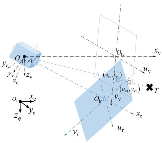
Figure 1. System framework and coordinate system diagram.

2.2. Quadrotor Model

$$\begin{array}{l}\dot{\mathit{p}}=\mathit{v}\\ \dot{\mathit{v}}=\mathit{g}+{\displaystyle \frac{1}{m}}(\mathit{F}+{\mathit{F}}_{\mathrm{d}})\\ {\dot{\mathit{R}}}_{\mathrm{b}}^{\mathrm{e}}={\mathit{R}}_{\mathrm{b}}^{\mathrm{e}}{\mathit{\omega }}_{\times }\\ \mathit{J}\dot{\mathit{\omega }}=\mathit{\tau }-\mathit{\omega }\times \mathit{J}\mathit{\omega }+{\mathit{\tau }}_d\end{array}$$

(1)

Here, $\mathit{p}={\left[\begin{array}{ccc}{p}_x& p_y& p_z\end{array}\right]}^{\mathrm{T}}$ and $\mathit{v}={\left[\begin{array}{ccc}{v}_x& v_y& v_z\end{array}\right]}^{\mathrm{T}}$ denote the velocity and position of the quadrotor in the Earth-fixed coordinate system, respectively, satisfying $\mathit{v}={\mathit{R}}_b^e{\mathrm{v}}_{\mathrm{b}}$, where ${\mathit{v}}_{\mathrm{b}}={\left[\begin{array}{ccc}{v}_{\mathrm{b}x}& v_{\mathrm{b}y}& v_{\mathrm{b}z}\end{array}\right]}^{\mathrm{T}}$ represents the velocity of the quadrotor in the BCS. $\mathit{g}={\left[\begin{array}{ccc}0& 0& g_G\end{array}\right]}^{\mathrm{T}}$ and $g_G$ denotes the gravitational constant. ${\mathit{R}}_b^e\in {ℝ}^{3\times 3}$ denotes the rotation matrix from the BCS to the ECS. $\mathit{\omega }={\left[\begin{array}{ccc}{\omega }_x& {\omega }_y& {\omega }_z\end{array}\right]}^{\mathrm{T}}$ represents the angular velocity of the quadrotor, and ${\mathit{\omega }}_{\times }$ denotes the skew-symmetric matrix generated by $\mathit{\omega }$. $\mathit{F}\in {ℝ}^3$ and $\mathit{\tau }\in {ℝ}^3$ denote the thrust force and torque, respectively, while ${\mathit{F}}_{\mathrm{d}}\in {ℝ}^3$ and ${\mathit{\tau }}_{\mathrm{d}}\in {ℝ}^3$ represent the disturbance force and disturbance torque, respectively. Additionally, $m\in ℝ$ and $\mathit{J}\in {ℝ}^{3\times 3}$ denote the mass and moment of inertia of the quadrotor, respectively.

2.3. IBVS Framework

For clarity of presentation, it is assumed that the CCS coincides with the BCS of the quadrotor, leading to the relation ${\mathit{v}}_{\mathrm{c}}={\mathit{v}}_{\mathrm{b}}$. A pinhole camera model is adopted, where the image-space position of quadrotor $i$ is given by $\mathit{s}={\left[\begin{array}{cc}u& v\end{array}\right]}^{\mathrm{T}}={\left[\begin{array}{cc}f{p}_{\mathrm{c}y}/p_{\mathrm{c}x}& f{p}_{\mathrm{c}z}/p_{\mathrm{c}x}\end{array}\right]}^{\mathrm{T}}$. Here, $f$ denotes the camera focal length, and ${\mathit{p}}_{\mathrm{c}}={\left[\begin{array}{ccc}{p}_{\mathrm{c}x}& p_{\mathrm{c}y}& p_{\mathrm{c}z}\end{array}\right]}^{\mathrm{T}}$ represents the relative position in the camera frame. Based on its position in the ECS, the dynamics of the image feature $\dot{\mathit{s}}$ can be expressed via the interaction matrix ${\mathit{L}}_{s\mathrm{r}}\in {ℝ}^{2\times 6}$ [29] and the velocity vector ${\mathit{v}}_{s\mathrm{r}}={\left[\begin{array}{cc}{v}_{\mathrm{c}}^{\mathrm{T}}& {\omega }^{\mathrm{T}}\end{array}\right]}^{\mathrm{T}}$ as follows:

$$\dot{\mathit{s}}={\mathit{L}}_{s\mathrm{r}}{\mathit{v}}_{s\mathrm{r}}$$

(2)

The specific form of ${\mathit{L}}_{s\mathrm{r}}$ is given as follows:

$${\mathit{L}}_{s\mathrm{r}}=\left[\begin{array}{cccccc}{\displaystyle \frac{u}{p_{\mathrm{c}x}}}& -{\displaystyle \frac{f}{p_{\mathrm{c}x}}}& 0& v& -{\displaystyle \frac{f^2+u^2}{f}}& {\displaystyle \frac{uv}{f}}\\ {\displaystyle \frac{v}{p_{\mathrm{c}x}}}& 0& -{\displaystyle \frac{f}{p_{\mathrm{c}x}}}& -u& {\displaystyle \frac{f^2+v^2}{f}}& -{\displaystyle \frac{uv}{f}}\end{array}\right]$$

The desired relative position in the ECS corresponds to the desired position ${\mathit{s}}^{\ast }$ in the image space. The IBVS control law is typically designed as ${\mathit{v}}_{\mathrm{rd}}=-\gamma {\widehat{\mathit{L}}}_{sr}^{+}(\mathit{s}-{\mathit{s}}^{\ast })$, where $\gamma >0$ is a gain coefficient, ${\mathit{L}}_{sr}^{+}$ denotes the Moore–Penrose inverse of ${\mathit{L}}_{s\mathrm{r}}$, and the depth information $p_{\mathrm{c}x}$ required in ${\mathit{L}}_{s\mathrm{r}}$ needs to be estimated. Even under large initial error conditions, this control law can achieve local asymptotic stability of the closed-loop system [30], i.e., $\mathit{s}\to {\mathit{s}}^{\ast }$.

Since the quadrotor is an underactuated system, to decouple the coupling effects of pitch and roll motions on translational motion, the following image model is established based on a virtual camera system:

$${\dot{\mathit{s}}}_{\mathrm{v}}=\left[\begin{array}{c}{\dot{u}}_{\mathrm{v}}\\ {\dot{v}}_{\mathrm{v}}\end{array}\right]={\mathit{L}}_{s\mathrm{v}}{\mathit{v}}_{sv}=\left[\begin{array}{cccc}-{\displaystyle \frac{u_{\mathrm{v}}}{p_{\mathrm{v}x}}}& {\displaystyle \frac{f}{p_{\mathrm{v}x}}}& 0& {\displaystyle \frac{f^2+u_{\mathrm{v}}^2}{f}}\\ -{\displaystyle \frac{v_{\mathrm{v}}}{p_{\mathrm{v}x}}}& 0& {\displaystyle \frac{f}{p_{\mathrm{v}x}}}& {\displaystyle \frac{u_{\mathrm{v}}{v}_{\mathrm{v}}}{f}}\end{array}\right]\left[\begin{array}{c}{v}_{\mathrm{v}x}\\ v_{\mathrm{v}y}\\ v_{\mathrm{c}z}\\ {\omega }_z\end{array}\right]$$

(3)

where ${\mathit{p}}_{\mathrm{v}}={\left[\begin{array}{ccc}{p}_{\mathrm{v}x}& p_{\mathrm{v}y}& p_{\mathrm{v}z}\end{array}\right]}^{\mathrm{T}}$ denotes the relative position vector in the VCS, and velocity vector ${\mathit{v}}_{s\mathrm{v}}={\left[\begin{array}{cc}{\mathit{v}}_{\mathrm{v}}^{\mathrm{T}}& {\omega }_z\end{array}\right]}^{\mathrm{T}}$, where ${\mathit{v}}_{\mathrm{v}}$ represents the velocity in the VCS. Therefore, ${\mathit{v}}_{\mathrm{vd}}=-\gamma {\widehat{\mathit{L}}}_{s\mathrm{v}}^{+}(\mathit{s}-{\mathit{s}}^{\ast })$ can be adopted as the control law based on the selected image model.

2.4. Basic Concepts of Graph Theory

A graph $\mathcal{G}$ consists of a vertex set $\mathcal{V}\left(\mathcal{G}\right)$ and an edge set $\mathcal{E}\left(\mathcal{G}\right)$, representing the communication relationships among nodes in this paper, where each node corresponds to a quadrotor. The set of neighboring nodes of vertex $i$ is denoted as ${\mathcal{N}}_i\left(\mathcal{G}\right)\triangleq \left\{j\in \mathcal{V}|\left(i,j\right)\in \mathcal{E}\left(\mathcal{G}\right)\right\}$. The Laplacian matrix of graph $\mathcal{G}$ is defined as $\mathcal{L}\left(\mathcal{G}\right)\triangleq \mathit{D}-\mathit{A}\in {ℝ}^{N\times N}$, where $\mathit{A}={\left\{a_{ij}\right\}}_{N\times N}$ denotes the adjacency matrix of $\mathcal{G}$ with elements $a_{ij}=1$ if $i\ne j$ and $\left(i,j\right)\in \mathcal{E}\left(\mathcal{G}\right)$, and $a_{ij}=0$ otherwise. $\mathit{D}=\mathrm{diag}\left(d_1,\dots ,d_N\right)$ is the degree matrix with $d_i\triangleq {\displaystyle {\sum }_{j=1}^N{a}_{ij}}$. Since the graph considered in this paper is undirected, $\mathcal{L}\left(\mathcal{G}\right)$ is a symmetric positive semidefinite matrix [30].

Consider a multi- quadrotor system composed of N quadrotors (nodes), whose dynamic model is given by Equation (1). The joint state vector formed by the positions of all nodes is denoted as ${\mathit{p}}_q={[\begin{array}{ccc}{\mathit{p}}_1^{\mathrm{T}}& \dots & {\mathit{p}}_N^{\mathrm{T}}\end{array}]}^{\mathrm{T}}$, and the distance between any two nodes i and j is given by ${\delta }_{ij}=‖{\mathit{p}}_i-{\mathit{p}}_j‖$.

Assumption 1.

The graph $\mathcal{G}$ considered in this paper is connected.

2.5. Problem Statement

This paper aims to employ multiple quadrotors, modeled as in Equation (1), to achieve formation-based encirclement tracking control of an unknown maneuvering target.

In the image space, based on the IBVS control law, the image position of the maneuvering target is driven to converge to the center of the camera’s FOV, i.e., $\mathit{s}\to {\mathit{s}}^{\ast }$. Simultaneously, the image positions of quadrotors are predicted and marked within the FOV to prevent misidentifying a quadrotor as the maneuvering target.

In the ECS, through a distributed control scheme, the quadrotors are guided to form a uniformly distributed encircling formation around the target, i.e., ${\delta }_{ij}\to p_{\mathrm{d}}$, where $p_{\mathrm{d}}\in {ℝ}^{+}$ denotes the desired inter-agent distance. Meanwhile, collisions between quadrotors must be avoided, i.e., ${\delta }_{ij}>h_{\mathrm{c}}$, where $h_{\mathrm{c}}>0$ represents the safety distance.

3. Control Method Design

The proposed control framework is illustrated in Figure 2.

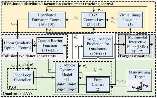
Figure 2. Schematic diagram of control system framework.

3.1. Target Velocity Estimation via IMM Filter

An Interacting Multiple Model (IMM) filter is a hybrid estimation framework that incorporates $m$ kinematic models, each corresponding to an independent Kalman Filter. The switching among the models is governed by a Markov chain, with model probabilities ${\mu }_k^j$ updated recursively over time [17].

The IMM filter generally operates in two phases: the filtering phase and the mixing phase. In the filtering phase, each filter performs prediction and update (the Kalman filtering process) on the state ${\widehat{\mathit{x}}}_{k-}^i$ based on its corresponding dynamic model and the current measurement ${\mathit{z}}_k$. In the mixing phase, the estimation results from all models are interactively fused according to their probabilities ${\mu }_k^{i|j}$. For each model $j$, the mixed initial state estimate ${\widehat{\mathit{x}}}_k^j$ and covariance ${\mathit{P}}_k^j$ are computed, preparing the initialization for the next filtering step. The specific procedure is given in Equation (4):

$$\begin{array}{l}{\widehat{\mathit{x}}}_k^j={\displaystyle \sum _{i=1}^m{\mu }_k^{i|j}{\widehat{\mathit{x}}}_{k-}^i}\\ {\mathit{P}}_k^j={\displaystyle \sum _{i=1}^m{\mu }_k^{i|j}\left({\mathit{P}}_{k-}^j+\left[{\widehat{\mathit{x}}}_k^i-{\widehat{\mathit{x}}}_k^j\right]{\left[{\widehat{\mathit{x}}}_k^i-{\widehat{\mathit{x}}}_k^j\right]}^{\mathrm{T}}\right)}\end{array}$$

(4)

Based on the likelihoods ${\mu }_k^j$ of each model, the overall state estimate ${\widehat{\mathit{x}}}_k$ and overall covariance ${\mathit{P}}_k$ are obtained by performing weighted fusion of the estimates from all models, as shown in Equation (5):

$$\begin{array}{l}{\widehat{\mathit{x}}}_k={\displaystyle \sum _{j=1}^m{\mu }_k^j{\widehat{\mathit{x}}}_k^j}\\ {\mathit{P}}_k={\displaystyle \sum _{j=1}^m{\mu }_k^j\left({\mathit{P}}_k^j+\left[{\widehat{\mathit{x}}}_{\mathit{k}}^j-{\widehat{\mathit{x}}}_k\right]{\left[{\widehat{\mathit{x}}}_k^i-{\widehat{\mathit{x}}}_k\right]}^{\mathrm{T}}\right)}\end{array}$$

(5)

For further details regarding the IMM framework, please refer to [31]. In this work, we adopt two motion models: the CV model and the CA model. The stochastic discrete-time state-space representation of the kinematic models is given by Equation (6):

$${\mathit{x}}_{k+1}=\mathit{A}{\mathit{x}}_k+{\mathit{n}}_{R,k},{\mathit{n}}_{R,k}~\mathcal{N}\left(0,\mathit{R}\right)$$

(6)

where $\mathit{x}$ is the state vector of the target, $\mathit{A}$ denotes the state transition matrix, ${\mathit{n}}_{R,k}$ represents zero-mean Gaussian process noise with covariance matrix $\mathit{R}$. For the measurement of the target position, multiple onboard cameras are employed for cooperative localization. A multi-view geometric linearized triangulation technique [32] is adopted, and the target position is estimated via least-squares fitting. The stochastic discrete-time state-space representation of the measurement model is given by Equation (7):

$${\mathit{z}}_{k+1}=\mathit{H}{\mathit{x}}_k+{\mathit{n}}_{Q,k},{\mathit{n}}_{Q,k}~\mathcal{N}\left(0,\mathit{Q}\right)$$

(7)

where $\mathit{z}\in {ℝ}^3$ is the measurement vector, $\mathit{H}$ denotes the measurement matrix, and ${\mathit{n}}_{Q,k}$ represents zero-mean Gaussian measurement noise with covariance matrix $\mathit{Q}={\sigma }_q{\mathit{I}}_3$. The CV and CA motion models can be derived from Equation (6), which follows a classical state transition process [17].

3.2. Formation Encirclement Controller Based on IBVS

As stated in the problem description in Section 2.5, a control law must be designed to achieve the control objectives in both the image space and the ECS.

$${\mathit{p}}_{\mathrm{vr},i}={\mathit{R}}_{\mathrm{e},i}^{\mathrm{v}}{\widehat{\mathit{p}}}_{\mathrm{r},i},i\in \left[\begin{array}{ccc}1& \dots & N\end{array}\right]$$

(8)

where ${\mathit{p}}_{\mathrm{vr},i}$ denotes the relative position in the VCS, the subscript $i$ represents the $i$-the quadrotor, ${\mathit{R}}_{\mathrm{e},i}^{\mathrm{v}}$ signifies the rotation matrix from the ECS to the VCS, and ${\widehat{\mathit{p}}}_{\mathrm{r},i}={\mathit{p}}_i-{\widehat{\mathit{p}}}_{\mathrm{t}}$ indicates the relative position in the ECS. The virtual image coordinates $u_{\mathrm{v},i}$, $v_{\mathrm{v},i}$ can be obtained through Equation (9):

$$\begin{array}{l}{u}_{\mathrm{v},i}={\displaystyle \frac{f}{{\mathit{p}}_{\mathrm{v}\mathrm{r},i}(1)}}{\mathit{p}}_{\mathrm{v}\mathrm{r},i}(2)\\ v_{\mathrm{v},i}={\displaystyle \frac{f}{{\mathit{p}}_{\mathrm{v}\mathrm{r},i}(1)}}{\mathit{p}}_{\mathrm{v}\mathrm{r},i}(3)\end{array}$$

(9)

The virtual image error is constructed as shown in Equation (10):

$${\mathit{e}}_{\mathrm{img},i}=\left[\begin{array}{c}{u}_{\mathrm{vd}}-u_{\mathrm{v},i}\\ v_{\mathrm{vd}}-v_{\mathrm{v},i}\end{array}\right]$$

(10)

where $u_{\mathrm{vd}}$ and $v_{\mathrm{vd}}$ denote the desired virtual image coordinates. The depth-direction error in the virtual camera coordinate system is constructed as Equation (11):

$$e_{\mathrm{dis},i}={\displaystyle \frac{2{\mathit{p}}_{\mathrm{v}\mathrm{r},i}(1)-\sqrt{2}{p}_{\mathrm{d}}}{\sqrt{2}{p}_{\mathrm{d}}}}$$

(11)

where $p_{\mathrm{d}}$ is the desired position error, which is designed here as a time-varying quantity. Let $p_{\mathrm{d}0}$ and $p_{\mathrm{d}1}$ denote the initial and final desired position errors, respectively, and let ${\xi }_{\mathrm{t}}$ represent the time decay rate. The expression for $p_{\mathrm{d}}$ is given by $p_{\mathrm{d}}=\left(p_{\mathrm{d}0}-p_{\mathrm{d}1}\right)\exp \left(-{\xi }_{\mathrm{t}}t\right)+p_{\mathrm{d}1}$.

The yaw-angle error is constructed as Equation (12):

$$e_{\psi ,i}={\psi }_{\mathrm{d},i}-{\psi }_i$$

(12)

Combining (9)–(12), the error vector ${\mathit{e}}_i$ is obtained as shown in Equation (13):

$${\mathit{e}}_i={\left[\begin{array}{ccc}{e}_{\mathrm{dis},i}& {\mathit{e}}_{\mathrm{img},i}^{\mathrm{T}}& e_{\psi ,i}\end{array}\right]}^{\mathrm{T}}$$

(13)

Based on (3) and (13), the control law in the image space is designed as follows:

$${\mathit{v}}_{\mathrm{v},i}=-{\lambda }_{\mathrm{v},i}{\widehat{\mathit{L}}}_{\mathrm{v},i}^{+}{\mathit{e}}_i$$

(14)

where ${\lambda }_{\mathrm{v},i}\in {ℝ}^{+}$ is the control gain coefficient, ${\mathit{v}}_{\mathrm{v},i}\left(4\right)$ denotes the fourth element of vector ${\mathit{v}}_{\mathrm{v},i}$, representing the desired yaw angular rate that can be directly used as the input to the attitude control loop. ${\widehat{\mathit{L}}}_{\mathrm{v},i}^{+}$ denotes the Moore–Penrose pseudoinverse of ${\widehat{\mathit{L}}}_{\mathrm{v},i}$, whose explicit form is given by Equation (15):

$${\widehat{\mathit{L}}}_{\mathrm{v},i}=\left[\begin{array}{cccc}{\displaystyle \frac{-\sqrt{2}}{p_{\mathrm{d}}}}& 0& 0& {\displaystyle \frac{-\sqrt{2}{\mathit{p}}_{\mathrm{v}\mathrm{r},i}(2)}{p_{\mathrm{d}}}}\\ {\displaystyle \frac{-u_{\mathrm{v},i}}{{\widehat{\mathit{p}}}_{\mathrm{v}\mathrm{r},i}(1)}}& {\displaystyle \frac{f}{{\widehat{\mathit{p}}}_{\mathrm{v}\mathrm{r},i}(1)}}& 0& {\displaystyle \frac{f^2+u_{\mathrm{v},i}^2}{f}}\\ {\displaystyle \frac{-v_{\mathrm{v},i}}{{\widehat{\mathit{p}}}_{\mathrm{v}r,i}(1)}}& 0& {\displaystyle \frac{f}{{\widehat{\mathit{p}}}_{\mathrm{v}\mathrm{r},i}(1)}}& {\displaystyle \frac{u_{\mathrm{v},i}{v}_{\mathrm{v},i}}{f}}\\ 0& 0& 0& -1\end{array}\right]$$

(15)

From Equation (15), it can be observed that ${\widehat{\mathit{L}}}_{\mathrm{v},i}$ is non-singular. Inspired by [33], the position error of each node is formulated as Equation (16):

$${\mathit{e}}_{\mathrm{rel},i}={\displaystyle \sum _{j\in {\mathcal{N}}_i\left(\mathcal{G}\right)}(‖{\mathit{p}}_j-{\mathit{p}}_i‖}-{\displaystyle \frac{p_{\mathrm{d}}}{\sqrt{2}}})\cdot {\displaystyle \frac{{\mathit{p}}_j-{\mathit{p}}_i}{‖{\mathit{p}}_j-{\mathit{p}}_i‖}}$$

(16)

where $‖\cdot ‖$ denotes the Euclidean norm of a vector. By combining the expression of ${\mathit{p}}_q$ from Section 2.2 with Equation (13), we further derive Equation (17):

$${\mathit{e}}_{\mathrm{rel}}=\left(\mathcal{L}\otimes {\mathit{I}}_3\right){\mathit{p}}_q-{\displaystyle \frac{\sqrt{2}}{2}}D\left({\mathit{p}}_q\right)$$

(17)

where ${\mathit{e}}_{\mathrm{rel}}={\left[\begin{array}{ccc}{\mathit{e}}_{\mathrm{rel},1}& \dots & {\mathit{e}}_{\mathrm{rel},N}\end{array}\right]}^{\mathrm{T}}$ is the relative position error vector of all nodes, and $\otimes$ denotes the Kronecker product. Combining with Equation (14), the control law is designed as (18):

$${\mathit{v}}_{\mathrm{c},i}=-{\lambda }_{\mathrm{v},i}{\widehat{\mathit{L}}}_{\mathrm{v},i}^{+}\left(1:3,1:3\right){\mathit{e}}_i\left(1:3\right)+{\lambda }_{\mathrm{c},i}{\mathit{R}}_{\mathrm{e},i}^{\mathrm{v}}{\mathit{e}}_{\mathrm{rel},i}$$

(18)

where ${\lambda }_{\mathrm{c},i}\in {ℝ}^{+}$ is the control gain coefficient, ${\widehat{\mathcal{L}}}_{\mathrm{v},i}^{+}\left(1:3,1:3\right)$ denotes the submatrix formed by the first three rows and three columns of ${\widehat{\mathit{L}}}_{\mathrm{v},i}^{+}$, and ${\mathit{e}}_i\left(1:3\right)$ represents the vector containing the first three elements of ${\mathit{e}}_i$. Incorporating the estimated target velocity ${\widehat{\mathit{v}}}_{\mathrm{t}}$ obtained from the IMM filter in Section 3.1 and performing coordinate transformation, the desired control input is given by:

$${\mathit{v}}_{\mathrm{con},i}={\mathit{R}}_{\mathrm{v}}^{\mathrm{e}}\left(v_{\mathrm{c},i}+{\mathit{R}}_{\mathrm{e}}^{\mathrm{v}}{\widehat{\mathit{v}}}_{\mathrm{t}}\right)$$

(19)

Lemma 1.

According to LaSalle’s invariance principle, if a system $\dot{x}=f\left(x\right)$ is locally Lipschitz and there exists a continuously differentiable positive-definite function  $V\left(x\right)|\mathcal{D}\subset {ℝ}^n$ such that $\dot{V}\left(x\right)\le 0$ for all $x\in \mathcal{D}$. Let $\Omega =\left\{x\in \mathcal{D}|\dot{V}\left(x\right)=0\right\}$ and let $\mathcal{M}$ be the largest invariant set in $\Omega$. Then every trajectory $x\left(t\right)$ starting in $\mathcal{D}$ approaches $\mathcal{M}$ as $t\to \infty$.

Let $V_{rel}={\displaystyle \raisebox{1ex}{$1$}\!\left/ \!\raisebox{-1ex}{$4$}\right.}{\displaystyle {\sum }_{i\ne j}{\left(\left({\mathit{p}}_j-{\mathit{p}}_i\right)-p_d\right)}^2}$ and ${\mathit{H}}_{ij}={\partial }^2{V}_{\mathrm{rel}}/\partial {\mathit{p}}_i\partial {\mathit{p}}_j$. The Hessian matrix $\mathcal{H}\in {ℝ}^{3\mathrm{m} \times 3\mathrm{m}}$ is defined as symmetric and positive semidefinite, where its block ${\left(i,j\right)}_{i,j\in \left[1,N\right]}$ is given by ${\mathit{H}}_{ij}$. Let $h_{\min }>0$ and $h_{\max }>0$ denote the minimum eigenvalue ${\lambda }_{\min }\left(\mathcal{H}\right)$ and the maximum eigenvalue ${\lambda }_{\max }\left(\mathcal{H}\right)$ of $\mathcal{H}$, respectively. Furthermore, let $\mathcal{L}=\mathrm{diag}\left(\begin{array}{ccc}{\mathit{L}}_{s,1}& \dots & {\mathit{L}}_{s,m}\end{array}\right)$ and ${\mathcal{L}}^{-1}=\mathrm{diag}\left(\begin{array}{ccc}{\mathit{L}}_{s,1}^{-1}& \dots & {\mathit{L}}_{s,m}^{-1}\end{array}\right)$, where ${\mathit{L}}_{s,i}$ represents ${\widehat{\mathit{L}}}_{\mathrm{v},i}^{+}\left(1:3,1:3\right)$.

Assumption 2.

The norms of the block matrix $\mathcal{L}$ and its pseudo-inverse ${\mathcal{L}}^{-1}$, denoted as $A=‖\mathcal{L}‖$and $B=‖{\mathcal{L}}^{-1}‖$, respectively, satisfy $AB>1$. Furthermore, there exists $\eta \in [(q+\sqrt{q^2+4pg})/2p,\min \left(\begin{array}{cc}\alpha /h_{\max }B& \beta h_{\min }/A\end{array}\right)]$, where $p=h_{\max }(AB-1)$, $g=\alpha \beta \left(h_{\max }AB-h_{\min }\right)$, $q=\alpha \left(A+h_{\max }\right)+\beta h_{\max }B(h_{\min }+A)$, $\alpha >0$ and $\beta >0$.

Theorem 1.

Under Assumptions 1 and 2, the control law given by Equation (19) simultaneously achieves convergence of the image error in the image space and convergence of the formation error in the ECS. The proof is as follows:

Proof. 

Combining Equations (14) and (16), let ${\mathit{a}}_i={\mathit{e}}_i\left(1:3\right)$ and ${\mathit{b}}_i={\mathit{e}}_{\mathrm{rel},i}$. Substituting these into Equation (18) yields:

$${\dot{\mathit{a}}}_i=-{\lambda }_{\mathrm{v}}{\mathit{a}}_i-{\lambda }_{\mathrm{c}}{\mathit{L}}_{s,i}{\mathit{b}}_i$$

(20)

Combining $V_{rel}={\displaystyle \raisebox{1ex}{$1$}\!\left/ \!\raisebox{-1ex}{$4$}\right.}{\displaystyle {\sum }_{i\ne j}{\left(‖{\mathit{p}}_j-{\mathit{p}}_i‖-p_d\right)}^2}$, we have ${\mathit{b}}_i=-{\nabla }_{p_i}{V}_{\mathrm{rel}}$. Thus, it follows that:

$${\dot{\mathit{b}}}_i=-{\nabla }_{{\mathit{p}}_i}^2{V}_{\mathrm{rel}}{\dot{\mathit{p}}}_i-{\displaystyle \sum _{j\ne i}\frac{{\partial }^2{V}_{\mathrm{rel}}}{\partial {\mathit{p}}_i\partial {\mathit{p}}_j}}{\dot{\mathit{p}}}_j$$

(21)

Linearizing around the equilibrium point, ${\dot{\mathit{b}}}_i$ can be approximated as:

$${\dot{\mathit{b}}}_i\approx -{\lambda }_{\mathrm{v}}{\mathit{H}}_{ii}{\mathit{L}}_{s,i}^{-1}{\mathit{a}}_i-{\lambda }_{\mathrm{c}}{\mathit{H}}_{ii}{\mathit{b}}_i-{\lambda }_{\mathrm{v}}{\displaystyle {\sum }_{j\ne i}{\mathit{H}}_{ij}{\mathit{L}}_{s,j}^{-1}{\mathit{a}}_j}-{\lambda }_{\mathrm{c}}{\displaystyle {\sum }_{j\ne i}{\mathit{H}}_{ij}{\mathit{b}}_j}$$

(22)

Let $\mathit{a}={\left[\begin{array}{ccc}{\mathit{a}}_1& \dots & {\mathit{a}}_N\end{array}\right]}^{\mathrm{T}}$, $\mathit{b}={\left[\begin{array}{ccc}{\mathit{b}}_1& \dots & {\mathit{b}}_N\end{array}\right]}^{\mathrm{T}}$. Based on the definition of the block matrix $\mathcal{L}$, and according to Equations (20)–(22), the following dynamic relationship holds:

$$\dot{\mathit{a}}=-{\lambda }_{\mathrm{v}}\mathit{a}-{\lambda }_{\mathrm{c}}\mathcal{L}\mathit{b}$$

$$\dot{\mathit{b}}=-{\lambda }_{\mathrm{v}}\mathcal{H}{\mathcal{L}}^{-1}\mathit{a}-{\lambda }_{\mathrm{c}}\mathcal{H}\mathit{b}$$

Consider the following Lyapunov function candidate:

$$V\left(\mathit{a},\mathit{b}\right)={\displaystyle \frac{1}{2}}\alpha {‖\mathit{a}‖}^2+{\displaystyle \frac{1}{2}}\beta {\mathit{b}}^{\mathrm{T}}{\mathcal{H}}^{-1}\mathit{b}+\eta {\mathit{a}}^{\mathrm{T}}\mathit{b}$$

From $V\left(\mathit{a},\mathit{b}\right)$, it can be observed that when $V\left(\mathit{a},\mathit{b}\right)=0$, it is equivalent to $\mathit{e}=\mathbf{0}$ and ${\mathit{e}}_{rel}=\mathbf{0}$, which implies that both the image-space error and the formation position error converge to zero.

According to the positive-definiteness condition:

$$\left[\begin{array}{cc}\alpha \mathit{I}& \eta \mathit{I}\\ \eta \mathit{I}& \beta {\mathcal{H}}^{-1}\end{array}\right]>0$$

This requires satisfying:

$$\beta >{\displaystyle \frac{{\eta }^2}{\alpha }}{h}_{\min }$$

(23)

Computing the derivative of $V\left(\mathit{a},\mathit{b}\right)$ yields:

$$\dot{V}\left(\mathit{a},\mathit{b}\right)=\alpha {\mathit{a}}^{\mathrm{T}}\dot{\mathit{a}}+\beta {\mathit{b}}^{\mathrm{T}}{\mathcal{H}}^{-1}\dot{\mathit{b}}+\eta {\dot{\mathit{a}}}^{\mathrm{T}}\mathit{b}+\eta {\mathit{a}}^{\mathrm{T}}\dot{\mathit{b}}$$

Substituting Equations (26) and (27) and rearranging into quadratic form:

$$\begin{array}{l}\dot{V}\left(\mathit{a},\mathit{b}\right)=-{\lambda }_{\mathrm{v}}\alpha {‖\mathit{a}‖}^2-{\lambda }_{\mathrm{c}}\beta {‖\mathit{b}‖}^2-\eta {\lambda }_{\mathrm{v}}{\mathit{a}}^{\mathrm{T}}\mathcal{H}{\mathcal{L}}^{-1}\mathit{a}-\eta {\lambda }_{\mathrm{c}}{\mathit{b}}^{\mathrm{T}}{\mathcal{L}}^{\mathrm{T}}\mathit{b}-\\ {\lambda }_{\mathrm{c}}\alpha {\mathit{a}}^{\mathrm{T}}{\mathcal{L}}^{\mathrm{T}}\mathit{b}-{\lambda }_{\mathrm{v}}\beta {\mathit{b}}^{\mathrm{T}}{\mathcal{L}}^{-\mathrm{T}}\mathit{a}-\eta {\lambda }_{\mathrm{v}}{\mathit{a}}^{\mathrm{T}}\mathit{b}-\eta {\lambda }_{\mathrm{c}}{\mathit{a}}^{\mathrm{T}}\mathcal{H}\mathit{b}\end{array}$$

(24)

Denoting $A=‖\mathcal{L}‖$ and $B=‖{\mathcal{L}}^{-1}‖$, an upper bound of $\dot{V}\left(\mathit{a},\mathit{b}\right)$ can be obtained:

$$\begin{array}{l}\dot{V}\left(\mathit{a},\mathit{b}\right)\le -{\lambda }_{\mathrm{v}}\left(\alpha -\left|\eta \right|h_{\max }B\right){‖\mathit{a}‖}^2-{\lambda }_{\mathrm{c}}\left(\beta h_{\min }-\left|\eta \right|A\right){‖\mathit{b}‖}^2+\\ \left[{\lambda }_{\mathrm{c}}\alpha A+{\lambda }_{\mathrm{v}}\beta h_{\max }B+\left|\eta \right|({\lambda }_{\mathrm{v}}+{\lambda }_{\mathrm{c}}{h}_{\max })\right]‖\mathit{a}‖‖\mathit{b}‖\end{array}$$

(25)

Let $p_{11}={\lambda }_{\mathrm{v}}\left(\alpha -\left|\eta \right|h_{\max }B\right)$,$p_{22}={\lambda }_{\mathrm{c}}\left(\beta h_{\min }-\left|\eta \right|A\right)$,$p_{12}={\displaystyle \raisebox{1ex}{$1$}\!\left/ \!\raisebox{-1ex}{$2$}\right.}\left[{\lambda }_{\mathrm{c}}\alpha A+{\lambda }_{\mathrm{v}}\beta h_{\max }B+\left|\eta \right|({\lambda }_{\mathrm{v}}+{\lambda }_{\mathrm{c}}{h}_{\max })\right]$,

$$\dot{V}\left(\mathit{a},\mathit{b}\right)\le -{\left[\begin{array}{c}‖\mathit{a}‖\\ ‖\mathit{b}‖\end{array}\right]}^{\mathrm{T}}\left[\begin{array}{cc}{p}_{11}& -p_{12}\\ -p_{12}& p_{22}\end{array}\right]\left[\begin{array}{c}‖\mathit{a}‖\\ ‖\mathit{b}‖\end{array}\right]$$

(26)

From Equation (26), it is required that conditions $\alpha >\left|\eta \right|h_{\max }B$ and $\beta h_{\min }>\left|\eta \right|A$ are satisfied. To ensure condition $p_{11}{p}_{22}>p_{12}^2$, the following must hold:

$$c_1{c}_2{\lambda }_{\mathrm{v}}{\lambda }_{\mathrm{c}}>{\displaystyle \frac{1}{4}}{\left(a{\lambda }_{\mathrm{v}}+b{\lambda }_{\mathrm{c}}\right)}^2$$

(27)

where $c_1=\alpha -\left|\eta \right|h_{\max }B>0$, $c_2=\beta h_{\min }-\left|\eta \right|A>0$, $a=\beta h_{\max }B+\left|\eta \right|$, $b=\alpha A+\left|\eta \right|h_{\max }$. Let $r={\lambda }_{\mathrm{v}}/{\lambda }_{\mathrm{c}}$, a quadratic inequality with respect to $r$ can be derived:

$$a^2{r}^2+\left(2ab-4c_1{c}_2\right)r+b^2<0$$

(28)

According to the discriminant of the quadratic equation and Assumption 2, the feasible range of $r$ is

$${\displaystyle \frac{4c_1{c}_2-2ab-4\sqrt{c_1{c}_2(c_1{c}_2-ab)}}{2a^2}}<r<{\displaystyle \frac{4c_1{c}_2-2ab+4\sqrt{c_1{c}_2(c_1{c}_2-ab)}}{2a^2}}$$

(29)

Rearranging the discriminant $\left(c_1{c}_2-ab\right)$ into a quadratic equation in terms of $\left|\eta \right|$

$$p{\left|\eta \right|}^{2}q\left|\eta \right|-g>0$$

(30)

According to the positive-definiteness conditions $\alpha >\left|\eta \right|h_{\max }B$ and $\beta h_{\min }>\left|\eta \right|A$, together with Assumption 2, there exist constants $\eta \in [(q+\sqrt{q^2+4pg})/2p,$ and $\min \left(\begin{array}{cc}\alpha /h_{\max }B& \beta h_{\min }/A\end{array}\right)]$ such that inequality (30) holds. Consequently, a feasible solution for $r$ in (29) exists, ensuring that (26) is negative semidefinite. Thus, Theorem 1 is proved. Furthermore, by invoking Lemma 1, the system is uniformly asymptotically stable. □

3.3. CBF-Based Collision Avoidance for Quadrotors

As mentioned in Section 2.3, during motion, collision avoidance among quadrotors must be guaranteed, i.e., ${\delta }_{ij}>h_{\mathrm{c}}$ must hold, where $h_{\mathrm{c}}$ denotes the minimum safe distance. Inspired by [34], we introduce a collision-avoidance constraint based on the CBF $h_{ij}$, with ${\mathit{s}}_i={\left[\begin{array}{cc}{\mathit{p}}_i^{\mathrm{T}}& {\mathit{v}}_i^{\mathrm{T}}\end{array}\right]}^{\mathrm{T}}$, and subsequently derive the admissible input set:

$${\mathcal{S}}_{ij}=\left\{({\mathit{s}}_i,{\mathit{s}}_j)|h_{ij}({\mathit{s}}_i,{\mathit{s}}_j)\ge 0\right\}$$

(31)

where the specific form of $h_{ij}$ is given by Equation (32):

$$h_{ij}=\sqrt{4u_m\left(‖\Delta {\mathit{p}}_{ij}‖-h_{\mathrm{c}}\right)}+{\displaystyle \frac{\Delta {\mathit{p}}_{ij}^{\mathrm{T}}}{‖\Delta {\mathit{p}}_{ij}‖}}\Delta {\mathit{v}}_{ij}$$

(32)

where $u_m$ denotes the maximum allowable velocity. The corresponding linear CBF constraint can then be derived as:

$$-\Delta {\mathit{p}}_{ij}^{\mathrm{T}}\Delta {\mathit{u}}_{ij}^{\mathrm{T}}\le {\alpha }_1{h}_{ij}^3‖\Delta {\mathit{p}}_{ij}‖-{\displaystyle \frac{{\left(\Delta {\mathit{v}}_{ij}^{\mathrm{T}}\Delta {\mathit{p}}_{ij}\right)}^2}{{‖\Delta {\mathit{p}}_{ij}‖}^2}}+{‖\Delta {\mathit{v}}_{ij}‖}^2+{\displaystyle \frac{2u_m\Delta {\mathit{v}}_{ij}^{\mathrm{T}}\Delta {\mathit{p}}_{ij}}{\sqrt{4u_m\left(‖\Delta {\mathit{p}}_{ij}‖-h_{\mathrm{c}}\right)}}}$$

(33)

where $\Delta {\mathit{u}}_{ij}={\mathit{v}}_{con,i}-{\mathit{v}}_{con,j}$. Substituting $f_{ij}$ for the right-hand side expression in inequality (33), it follows that $f_{ij}=f_{ji}$ must be satisfied. Constraint (33) can thus be rewritten as:

$$-\Delta {\mathit{p}}_{ij}^{\mathrm{T}}\Delta {\mathit{u}}_{ij}^{\mathrm{T}}\le f_{ij}$$

(34)

which can be further allocated to nodes $i$ and $j$, respectively, as:

$$-\Delta {\mathit{p}}_{ij}^{\mathrm{T}}{\mathit{v}}_{\mathrm{con},i}\le {\displaystyle \frac{f_{ij}}{2}},-\Delta {\mathit{p}}_{ij}^{\mathrm{T}}{\mathit{v}}_{\mathrm{con},j}\le {\displaystyle \frac{f_{ji}}{2}}$$

(35)

Based on the linear constraint in (35), the optimal control law for node $i$ is obtained as:

$$\begin{array}{l}{\mathit{v}}_{\mathrm{con},i}=\arg \underset{j\in {\mathcal{N}}_i}{\min } {\displaystyle \frac{1}{2}}{\mathit{v}}_{\mathrm{con},i}^{\mathrm{T}}{\mathit{v}}_{\mathrm{con},i}\\ \mathrm{s}.\mathrm{t}. \mathrm{C}1:{\dot{\mathit{s}}}_i=\mathit{A}{\mathit{s}}_i+\mathit{B}{\mathit{v}}_{\mathrm{oc},i}\\ \mathrm{C}2:-\Delta {\mathit{p}}_{ij}^{\mathrm{T}}{\mathit{v}}_{\mathrm{con},i}\le {\displaystyle \frac{f_{ij}}{2}},j\in {\mathcal{N}}_i\\ \mathrm{C}3:‖{\mathit{v}}_{\mathrm{con},i}‖\le u_m\end{array}$$

Assumption 3.

The quadrotor formation satisfies constraint ${\delta }_{ij}>h_{\mathrm{c}}$ at the initial time $t=0 \mathrm{s}$.

3.4. Image-Coordinate Prediction of Quadrotors in the Field of View

During the tracking of a maneuvering target, the formation motion may cause a member of the formation to appear within the FOV of a node, leading to potential misidentification as the target. Such misidentification can interfere with accurate target tracking control and degrade the precision and stability of state estimation. Therefore, it is necessary to incorporate the prediction and marking of quadrotor positions into the control process to avoid misidentification. Inspired by [35], we project the positions of cooperative quadrotor onto the image plane for labeling and eliminate potential false detections based on overlap analysis. Each node receives the position information of other cooperating nodes via the communication network. The procedure for calculating the image-plane position of the $j$-th neighboring quadrotor on the onboard camera of the $i$ -th quadrotor is described as follows:

$${\mathit{p}}_i^j={\mathit{R}}_{\mathrm{e}}^{\mathrm{c},i}\left({\mathit{p}}_j-{\mathit{p}}_i\right)$$

(36)

where ${\mathit{p}}_i^j$ denotes the position of quadrotor $j$ in the CCS of quadrotor $i$, and ${\mathit{R}}_{\mathrm{e}}^{\mathrm{c},i}$ is the rotation matrix from the ECS to the CCS of quadrotor $i$ Combining with Equation (9), the image-plane coordinates $u_i^j$ and $v_i^j$ can be further obtained through the camera model as:

$$\left[\begin{array}{c}{\widehat{u}}_i^j\\ {\widehat{v}}_i^j\end{array}\right]={\left[\begin{array}{cc}f{\displaystyle \frac{{\mathit{p}}_i^j(2)}{{\mathit{p}}_i^j(1)}}& f{\displaystyle \frac{{\mathit{p}}_i^j(3)}{{\mathit{p}}_i^j(1)}}\end{array}\right]}^{\mathrm{T}}$$

(37)

Similarly, the position of the target in the CCS $i$, denoted as ${\mathit{p}}_i^{\mathrm{t}}$, and its corresponding image-plane coordinates $u_i^{\mathrm{t}}$ and $v_i^{\mathrm{t}}$ can be obtained as:

$$\left[\begin{array}{c}{u}_i^{\mathrm{t}}\\ v_i^{\mathrm{t}}\end{array}\right]={\left[\begin{array}{cc}f{\displaystyle \frac{{\mathit{p}}_i^{\mathrm{t}}(2)}{{\mathit{p}}_i^{\mathrm{t}}(1)}}& f{\displaystyle \frac{{\mathit{p}}_i^{\mathrm{t}}(3)}{{\mathit{p}}_i^{\mathrm{t}}(1)}}\end{array}\right]}^{\mathrm{T}}$$

(38)

Taking the projected image coordinates $u_i^j$, $v_i^j$ as the center, we define a bounding box with a threshold radius $d_N$. When a moving point appears within the bounding box of radius $d_N$, it is labeled as a misidentified quadrotor. In special cases where the same moving point appears simultaneously in two intersecting bounding boxes, such scenarios are not analyzed or processed here but will be addressed in detail in future work.

4. Simulation Experiments

4.1. Position and Velocity Estimation of the Maneuvering Target

The initial position of the target is ${\mathit{p}}_{\mathrm{t}}={\left[\begin{array}{ccc}50 \mathrm{m}& 0 \mathrm{m}& -20 \mathrm{m}\end{array}\right]}^{\mathrm{T}}$, and its initial velocity is ${\mathit{v}}_{\mathrm{t}}={\left[\begin{array}{ccc}2 \mathrm{m}/\mathrm{s}& 1 \mathrm{m}/\mathrm{s}& 0.5 \mathrm{m}/\mathrm{s}\end{array}\right]}^{\mathrm{T}}$. At time $t=6.67$ s, the target acceleration is ${\mathit{a}}_{\mathrm{t}}={\left[\begin{array}{ccc}3 {\mathrm{m}/\mathrm{s}}^2& 2 {\mathrm{m}/\mathrm{s}}^2& 1 {\mathrm{m}/\mathrm{s}}^2\end{array}\right]}^{\mathrm{T}}$. At time $t=13.33$ s, the target acceleration switches to ${\mathit{a}}_{\mathrm{t}}={\left[\begin{array}{ccc}-2 {\mathrm{m}/\mathrm{s}}^2& -2 {\mathrm{m}/\mathrm{s}}^2& -2 {\mathrm{m}/\mathrm{s}}^2\end{array}\right]}^{\mathrm{T}}$.

In Table 1, MPE denotes mean positional error, MVE denotes mean velocity error, MAPE denotes mean absolute positional error, and MAVE denotes mean absolute velocity error. MPE and MVE are computed as the RMSE, while MAPE and MAVE are calculated as the mean absolute error.

Table 1. Root mean square error and mean absolute error of the estimation.

Estimation Methods	MPE (m)	MVE (m/s)	MAPE (m/s)	MAVE (m/s)
IMM	0.4998	1.5195	0.4579	1.3535
EKF	0.5840	2.0660	0.4583	1.7637

Figure 3a illustrates the estimated trajectory of the target, where the triangle marker denotes the starting point and the circle marker indicates the endpoint. Both the EKF and the IMM filter achieve stable estimation of the target’s changing position. As shown in Figure 3b, the IMM filter outperforms the EKF in terms of both position and velocity estimation errors. Based on the MPE and MVE data in Table 1, it is observed that for target position estimation, the IMM reduces the estimation bias by 14.4% compared to the EKF, while for target velocity estimation, the accuracy improvement reaches 26.5%. The accuracy metric employed here is the root mean square error (RMSE) between the estimated and actual values. The percentage improvement in estimation accuracy is calculated as per Equation (39).

$$p_{\mathrm{im}}={\displaystyle \frac{RMS{E}_{IMM}-RMS{E}_{EKF}}{RMS{E}_{EKF}}}\cdot 100\%$$

(39)

where $p_{\mathrm{im}}$ denotes the percentage of improvement, and $RMS{E}_{IMM}$ and $RMS{E}_{EKF}$ represent the RMSE corresponding to the IMM and EKF estimation methods, respectively.

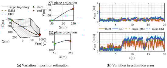
Figure 3. EKF and IMM estimation of target location.

Table 2 presents the instantaneous absolute estimation errors at the time instants of 1 s, 5 s, 10 s, 15 s, and 20 s. Table 3 summarizes the average absolute estimation errors over the intervals of 0–5 s, 5–10 s, 10–15 s, and 15–20 s.

Table 2. Instantaneous absolute error.

t (s)	Positional (m)		Velocity (m/s)
	IMM	EKF	IMM	EKF
1	0.3808	0.2536	0.3223	0.4065
5	0.4898	0.2720	0.6200	0.1376
10	0.6591	0.6965	2.0633	2.9200
15	0.2455	0.5201	0.7774	2.4286
20	0.5531	0.8371	1.5813	3.0512

Table 3. Average absolute error per interval.

t (s)	Positional (m)		Velocity (m/s)
	IMM	EKF	IMM	EKF
0–5	0.4459	0.4464	0.6754	0.4346
5–10	0.4221	0.4235	1.3766	1.5855
10–15	0.4750	0.4761	1.6717	2.3067
15–20	0.4885	0.4901	1.6901	2.7280

As shown in Table 2 and Table 3, the estimation performance of the IMM filter is comparable to that of the EKF when the target undergoes uniform linear motion. However, when the target exhibits accelerated motion, the IMM filter demonstrates superior estimation accuracy. These observations are further corroborated by the results presented in Figure 3b.

4.2. Simulation of Encirclement and Tracking Control of Mobile Targets

The target has an initial position ${\mathit{p}}_{\mathrm{t}}={\left[\begin{array}{ccc}50 \mathrm{m}& 0 \mathrm{m}& -20 \mathrm{m}\end{array}\right]}^{\mathrm{T}}$ and initial velocity ${\mathit{v}}_{\mathrm{t}}={\left[\begin{array}{ccc}3 \mathrm{m}/\mathrm{s}& 1.5 \mathrm{m}/\mathrm{s}& -0.6 \mathrm{m}/\mathrm{s}\end{array}\right]}^{\mathrm{T}}$. At time $t=10$ s, the target acceleration is ${\mathit{a}}_{\mathrm{t}}={\left[\begin{array}{ccc}0 {\mathrm{m}/\mathrm{s}}^2& 0.5 {\mathrm{m}/\mathrm{s}}^2& 0 {\mathrm{m}/\mathrm{s}}^2\end{array}\right]}^{\mathrm{T}}$. At $t=20$ s, the acceleration changes to ${\mathit{a}}_{\mathrm{t}}={\left[\begin{array}{ccc}0 {\mathrm{m}/\mathrm{s}}^2& -0.3 {\mathrm{m}/\mathrm{s}}^2& 0.06 {\mathrm{m}/\mathrm{s}}^2\end{array}\right]}^{\mathrm{T}}$ From $t=30$ s onward, the target maintains a constant velocity motion.

Four quadrotors, denoted as $Q_A$, $Q_B$, $Q_C$, and $Q_D$, are employed to perform encircling tracking of the target. Their respective initial positions are ${\mathit{p}}_A={\left[\begin{array}{ccc}0 \mathrm{m}& 0 \mathrm{m}& -1 \mathrm{m}\end{array}\right]}^{\mathrm{T}}$, ${\mathit{p}}_B={\left[\begin{array}{ccc}0.1 \mathrm{m}& 1 \mathrm{m}& -1 \mathrm{m}\end{array}\right]}^{\mathrm{T}}$, ${\mathit{p}}_C={\left[\begin{array}{ccc}-0.1 \mathrm{m}& 0 \mathrm{m}& 0 \mathrm{m}\end{array}\right]}^{\mathrm{T}}$, and ${\mathit{p}}_D={\left[\begin{array}{ccc}0.2 \mathrm{m}& 1 \mathrm{m}& 0 \mathrm{m}\end{array}\right]}^{\mathrm{T}}$, all with the same initial velocity $0 \mathrm{m}/\mathrm{s}$. The desired initial position offset $p_{\mathrm{d}0}$ and final position offset $p_{\mathrm{d}1}$ are set to 1 m and 0.3 m, respectively. The initial yaw angles of all quadrotors are $0 \mathrm{rad}$, while the desired yaw angles are ${\psi }_{\mathrm{d}A}=-\pi /4 \mathrm{rad}$, ${\psi }_{\mathrm{d}B}=\pi /4 \mathrm{rad}$, ${\psi }_{\mathrm{d}C}=-3\pi /4 \mathrm{rad}$, ${\psi }_{\mathrm{d}D}=3\pi /4 \mathrm{rad}$.

Figure 4 illustrates the tracking performance of the target using control methods based on PBVS and IBVS, respectively. Curves of different colors in the figure denote the flight trajectories of different quadrotors, with each color representing a single vehicle. Circular markers in the same color as a curve indicate the final position of the corresponding quadrotor. As shown in Figure 4, both methods are capable of achieving stable tracking of the target. The triangle in the figure represents the starting point of the formation and the target, the circle represents the final position of the formation, and the black square represents the final position of the target. From the enlarged view in Figure 4a, it can be observed that the formation successfully tracks the target. However, due to the high susceptibility of the PBVS method to noisy environments and its strong dependence on model accuracy, the formation fails to achieve a well-rounded encircling formation around the target during the tracking process, which deviates from our control objective. From Figure 4b, it can be observed that compared with the PBVS method, the IBVS-based control approach results in initially divergent trajectories among the quadrotors. This behavior arises because the IBVS-based control law is solved in the image space. Referring to the control law design process in Section 3.2, it can be noted that changes in yaw directly affect the error in the image space. Based on the current yaw angle and image error, a unique solution for the relative position with respect to the target in the ECS can be obtained. Consequently, while achieving the desired image position and yaw angle, an encircling formation around the target is generated. In the terminal tracking phase, the enlarged view in the figure shows the position distribution between the formation and the target, with arrows indicating the yaw direction of the quadrotor. This indicates that during the tracking process, the formation establishes and maintains an encircling configuration around the target.

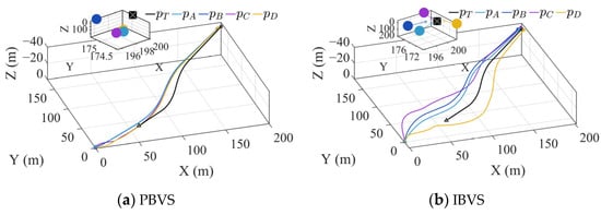
Figure 4. Encirclement and tracking engineering of a maneuvering target.

Figure 5 shows the variation in tracking error ${\mathit{e}}_p$ for quadrotors $Q_A$, $Q_B$, $Q_C$, and $Q_D$ relative to the target T using the PBVS and IBVS methods, respectively. The figure indicates that both methods achieve stable convergence of the tracking error. At $t=10 \mathrm{s}$ and $t=20 \mathrm{s}$, the tracking error exhibits noticeable fluctuations, which are attributed to changes in the target’s maneuverability at those instants. Within the same tracking period, the tracking error under the IBVS method is significantly smaller than that under PBVS. This is because the IBVS method relies directly on the image-space error, offering better robustness to noise and model uncertainties. In contrast, the PBVS method reconstructs a 3D relative position with respect to the target from 2D image information and then designs the control law based on this positional relationship. Consequently, noise and model uncertainties present in the 2D image space are amplified in the 3D space, directly degrading control accuracy. As seen in Figure 5c,d, during the initial tracking stage, the error along the y-axis ${\mathit{e}}_{py}$ is relatively large when using the IBVS method, which aligns with the formation-divergence behavior observed in Figure 4b. This occurs because the designed control law, which is based on the current image error and yaw angle, leads to an encircling motion trajectory around the target before the yaw angle converges to its desired value.

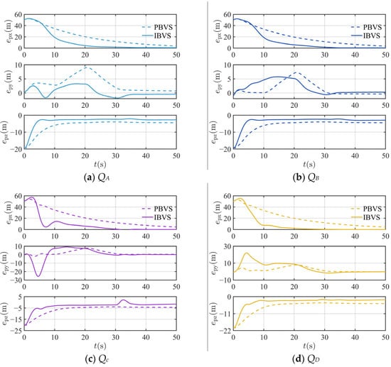
Figure 5. Position tracking error of maneuvering target.

Figure 6 illustrates the variation in relative distances among quadrotors within the formation, both before and after the introduction of CBF-based collision-avoidance constraints. In the figure, the dashed lines labeled $\left(i,j\right),i,j\in \left\{\begin{array}{cccc}A& B& C& D\end{array}\right\}, i\ne j$ represent the relative distance curves between quadrotors $Q_i$ and $Q_j$ without CBF, while the solid lines labeled $i_{\mathrm{c}}{j}_{\mathrm{c}}$ denote the corresponding curves after CBF is applied. The red dotted line near the bottom indicates the minimum safe distance $h_{\mathrm{c}}$ defined in the CBF framework: a collision is considered to occur if the relative distance ${\delta }_{ij}<h_{\mathrm{c}}$ between any two quadrotors falls below $h_{\mathrm{c}}$. From the figure, it can be seen that in the final stage of encirclement tracking, the introduction of CBF effectively ensures that the distance between all quadrotors remains above the safety threshold $h_{\mathrm{c}}$. In contrast, the curve $BC$ without CBF shows the occurrence of collisions (as shown in bold between 35 s and 40 s in the figure).

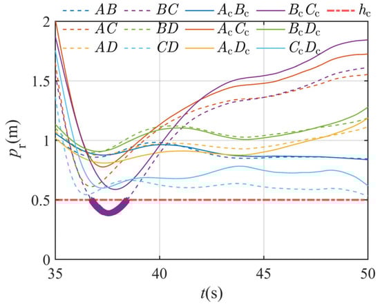
Figure 6. Changes in relative position before and after introducing collision avoidance constraints.

Figure 7 illustrates the FOV schematic of the onboard strapdown camera mounted on $Q_A$. Subfigures (a)–(f) show the FOV status at $t=1 \mathrm{s}$. $9 \mathrm{s}$, $19 \mathrm{s}$, $29 \mathrm{s}$, $39 \mathrm{s}$ and $49 \mathrm{s}$, respectively. The dots in the figure denote the quadrotors of the formation visible in the FOV, labeled as $Q_i$, $i\in \left\{\begin{array}{cccc}A& B& C& D\end{array}\right\}$. The cross symbol $\times$ marks the position of the target within the FOV. The dashed circles represent the identification markers for the formation quadrotors, denoted as $M_i$. As can be observed, during the tracking process, each quadrotor can predict the image positions of other formation members in its own FOV by utilizing its own attitude and the communicated position information of other quadrotors. This allows the target to be distinguished from multiple moving objects when they appear simultaneously in the FOV, thereby preventing estimation errors and control disruptions caused by misidentification. Furthermore, the figure confirms that the proposed image-space-based control method successfully maintains the target near the center of the FOV throughout the tracking process.

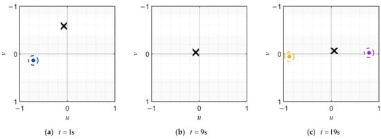
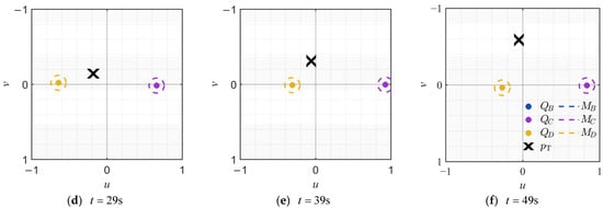
Figure 7. Dynamic changes in the position of moving objects within $Q_A$’s FOV.

5. Conclusions

This paper addresses the formation-based encirclement control of an unknown maneuvering target by proposing an IMM filter for target state estimation and a distributed IBVS formation control method for target encircling and tracking. Based on the RMSE metric, the simulation results show that the proposed estimation method achieves a 26.5% improvement in target state estimation accuracy compared to existing methods. The stability of the proposed control scheme is rigorously analyzed using Lyapunov theory. Compared to existing control methods, the distributed IBVS-based formation control not only achieves stable encircling and tracking of the target but also further reduces tracking errors. The introduced collision-avoidance constraints effectively prevent inter-agent collisions during formation control, thereby enhancing operational safety. Furthermore, the integrated prediction of other formation members within the FOV enables reliable distinction between the target and cooperative agents, mitigating estimation errors and control disruptions caused by misidentification. Meanwhile, the proposed control law successfully drives the image position of the target toward the center of the FOV.

References

- Li, Q.; Lu, X.; Wang, Y. A Novel Hierarchical Distributed Robust Formation Control Strategy for Multiple Quadrotor Aircrafts. IEEE Trans. Syst. Man Cybern. Syst. 2025, 55, 6450–6462. [Google Scholar] [CrossRef]
- Liu, K.; Yang, W.; Jiao, L.; Yuan, Z.; Wen, C.Y. Fast Fixed-Time Distributed Neural Formation Control-based Disturbance Observer for Multiple Quadrotor UAVs Under Unknown Disturbances. IEEE Trans. Aerosp. Electron. Syst. 2025, 61, 13137–13155. [Google Scholar] [CrossRef]
- Huang, Y.; Xu, X.; Meng, Z.; Sun, J. A Smooth Distributed Formation Control Method for Quadrotor UAVs Under Event-Triggering Mechanism and Switching Topologies. IEEE Trans. Vehic. Technol. 2025, 74, 10081–10091. [Google Scholar] [CrossRef]
- Liu, H.; Li, B.; Ahn, C.K. Asymptotically stable learning-based formation control for multi-quadrotor UAVs. IEEE Internet Things J. 2025, 12, 24985–24995. [Google Scholar] [CrossRef]
- Doakhan, M.; Kabganian, M.; Azimi, A. Aerial Payload Transportation with Energy-Efficient Flexible Formation Control of Quadrotors. Eur. J. Control 2025, 86, 101406. [Google Scholar] [CrossRef]
- Upadhyay, J.; Rawat, A.; Deb, D. Multiple drone navigation and formation using selective target tracking-based computer vision. Electronics 2021, 10, 2125. [Google Scholar] [CrossRef]
- Seidaliyeva, U.; Ilipbayeva, L.; Taissariyeva, K.; Smailov, N.; Matson, E.T. Advances and Challenges in Drone Detection and Classification Techniques: A State-of-the-Art Review. Sensors 2024, 24, 125. [Google Scholar] [CrossRef] [PubMed]
- García, M.; Caballero, R.; González, F.; Viguria, A.; Ollero, A. Autonomous drone with ability to track and capture an aerial target. In Proceedings of the 2020 International Conference on Unmanned Aircraft Systems (ICUAS), Athens, Greece, 1–4 September 2020; IEEE: New York, NY, USA, 2020; pp. 32–40. [Google Scholar]
- Yang, L.; Wang, X.; Liu, Z.; Shen, L. Robust Online Predictive Visual Servoing for Autonomous Landing of a Rotor UAV. IEEE Trans. Intell. Veh. 2025, 10, 2818–2835. [Google Scholar] [CrossRef]
- Li, W.; Ma, Y.; Zhang, Y.; Li, B.; Shi, Y.; Chu, L. A Multiangle Observation and Imaging Method for UAV Swarm SAR Based on Consensus Constraints. IEEE Sens. J. 2025, 25, 19776–19793. [Google Scholar] [CrossRef]
- Yang, K.; Bai, C.; Quan, Q. Multiview Target Estimation for Multicopter Swarm Interception. IEEE Trans. Instrum. Meas. 2025, 74, 5023312. [Google Scholar] [CrossRef]
- Tao, Y.; Chen, S.; Huo, X. Image-Based Visual Servo Control of a Quadrotor under Field of View Constraints Using a Pan-Tilt Camera. In Proceedings of the 39th Chinese Control Conference (CCC), Shenyang, China, 27–29 July 2020; IEEE: New York, NY, USA, 2020; pp. 3518–3523. [Google Scholar]
- Lin, F.; Peng, K.; Dong, X.; Zhao, S.; Chen, B.M. Vision-based formation for UAVs. In Proceedings of the 11th IEEE International Conference on Control & Automation (ICCA), Taichung, Taiwan, 18–20 June 2014; IEEE: New York, NY, USA, 2014; pp. 1375–1380. [Google Scholar]
- Vrba, M.; Stasinchuk, Y.; Báča, T.; Spurný, V.; Petrlík, M.; Heřt, D.; Žaitlík, D.; Saska, M. Autonomous capture of agile flying objects using UAVs: The MBZIRC 2020 challenge. Rob. Auton. Syst. 2022, 149, 103970. [Google Scholar] [CrossRef]
- Ma, J.; Chen, P.; Xiong, X.; Zhang, L.; Yu, S.; Zhang, D. Research on vision-based servoing and trajectory prediction strategy for capturing illegal drones. Drones 2024, 8, 127. [Google Scholar] [CrossRef]
- Su, Y.X.; Zheng, C.H.; Müller, P.C.; Duan, B.Y. A simple improved velocity estimation for low-speed regions based on position measurements only. IEEE Trans. Control Syst. Technol. 2006, 14, 937–942. [Google Scholar] [CrossRef]
- Pliska, M.; Vrba, M.; Báča, T.; Saska, M. Towards safe mid-air drone interception: Strategies for tracking & capture. IEEE Robot. Autom. Lett. 2024, 10, 8810–8817. [Google Scholar] [CrossRef]
- Fan, X.; Wang, G.; Han, J.; Wang, Y. Interacting multiple model based on maximum correntropy Kalman filter. IEEE Trans. Circuits Syst. II Exp. Briefs 2021, 68, 3017–3021. [Google Scholar] [CrossRef]
- Yunita, M.; Suryana, J.; Izzuddin, A. Error performance analysis of IMM-Kalman filter for maneuvering target tracking application. In Proceedings of the 2020 6th International Conference on Wireless and Telematics (ICWT), Yogyakarta, Indonesia, 3–4 September 2020; IEEE: New York, NY, USA, 2020; pp. 1–6. [Google Scholar]
- Leomanni, M.; Ferrante, F.; Dionigi, A.; Costante, G.; Valigi, P.; Fravolini, M.L. Quadrotor Control System Design for Robust Monocular Visual Tracking. IEEE Trans. Control Syst. Technol. 2024, 32, 1995–2008. [Google Scholar] [CrossRef]
- Lin, J.; Miao, Z.; Wang, Y.; Wang, H.; Wang, X.; Fierro, R. Vision-Based Safety-Critical Landing Control of Quadrotors with External Uncertainties and Collision Avoidance. IEEE Trans. Control Syst. Technol. 2024, 32, 1310–1322. [Google Scholar] [CrossRef]
- Zhao, W.; Liu, H.; Lewis, F.L.; Valavanis, K.P.; Wang, X. Robust Visual Servoing Control for Ground Target Tracking of Quadrotors. IEEE Trans. Control Syst. Technol. 2019, 28, 1980–1987. [Google Scholar] [CrossRef]
- Bastourous, M.; Al-Tuwayyij, J.; Guérin, F.; Guinand, F. Image based visual servoing for multi aerial robots formation. In Proceedings of the 28th Mediterranean Conference on Control and Automation (MED), Saint-Raphaël, France, 15–18 September 2020; IEEE: New York, NY, USA, 2020; pp. 115–120. [Google Scholar]
- Wang, C.; Sun, Y.; Ma, X.; Chen, Q.; Gao, Q.; Liu, X. Multi-agent dynamic formation interception control based on rigid graph. Complex Intell. Syst. 2024, 10, 5585–5598. [Google Scholar] [CrossRef]
- Karras, G.C.; Bechlioulis, C.P.; Fourlas, G.K.; Kyriakopoulos, K.J. Formation control and target interception for multiple multi-rotor aerial vehicles. In Proceedings of the 2020 International Conference on Unmanned Aircraft Systems (ICUAS), Athens, Greece, 1–4 September 2020; IEEE: New York, NY, USA, 2020; pp. 85–92. [Google Scholar]
- Rothe, J.; Strohmeier, M.; Montenegro, S. Autonomous Multi-UAV Net Defense System for Aerial Drone Interception. In Proceedings of the 2025 10th International Conference on Control and Robotics Engineering (ICCRE), Nagoya, Japan, 9–11 May 2025; IEEE: New York, NY, USA, 2025; pp. 171–177. [Google Scholar]
- Wu, A.; Yang, R.; Li, H.; Lv, M. A specified-time cooperative optimal control approach to unmanned aerial vehicle swarms. In Proceedings of the 2023 9th International Conference on Control, Automation and Robotics (ICCAR), Beijing, China, 21–23 April 2023; IEEE: New York, NY, USA, 2023; pp. 163–169. [Google Scholar]
- Montijano, E.; Cristofalo, E.; Zhou, D.; Schwager, M.; Sagues, C. Vision-based distributed formation control without an external positioning system. IEEE Trans. Robot. 2016, 32, 339–351. [Google Scholar] [CrossRef]
- Chaumette, F.; Hutchinson, S. Visual servo control. I. Basic approaches. IEEE Robot. Autom. Mag. 2006, 13, 82–90. [Google Scholar] [CrossRef]
- Chavez-Aparicio, E.I.; Becerra, H.M.; Hayet, J.B. A Novel Consensus-Based Formation Control Scheme in the Image Space. IEEE Control Syst. Lett. 2024, 8, 2769–2774. [Google Scholar] [CrossRef]
- Li, X.R.; Jilkov, V.P. Survey of maneuvering target tracking. Part V. Multiple-model methods. IEEE Trans. Aerosp. Electron. Syst. 2005, 41, 1255–1321. [Google Scholar] [CrossRef]
- Lee, J.; Lee, D.; Wang, Z.; Wong, K.C.; So, S. Vision-based position and velocity estimation of an intruder drone by multiple detector drones. In Proceedings of the Asia Pacific International Symposium On Aerospace Technology (APISAT 2024), Adelaide, South Australia, 5–8 November 2024; pp. 1748–1754. [Google Scholar]
- Xu, Y.; Qu, Y.; Luo, D.; Duan, H.; Guo, Z. Distributed predefined-time estimator-based affine formation target-enclosing maneuver control for cooperative underactuated quadrotor UAVs with fault-tolerant capabilities. Chin. J. Aeronaut. 2025, 38, 103042. [Google Scholar] [CrossRef]
- Wang, L.; Ames, A.D.; Egerstedt, M. Safety barrier certificates for collisions-free multirobot systems. IEEE Trans. Robot. 2017, 33, 661–674. [Google Scholar] [CrossRef]
- Zheng, C.; Mi, Y.; Guo, H.; Chen, H.; Zhao, S. Vision-Based Cooperative MAV-Capturing-MAV. arXiv 2025, arXiv:2503.06412. [Google Scholar] [CrossRef]
Disclaimer/Publisher’s Note: The statements, opinions and data contained in all publications are solely those of the individual author(s) and contributor(s) and not of MDPI and/or the editor(s). MDPI and/or the editor(s) disclaim responsibility for any injury to people or property resulting from any ideas, methods, instructions or products referred to in the content. |
© 2026 by the authors. Licensee MDPI, Basel, Switzerland. This article is an open access article distributed under the terms and conditions of the Creative Commons Attribution (CC BY) license.