A Fast Robust Integrated Guidance and Control Scheme for Flight Vehicles Based on Convergence Rate Estimation Mechanism

Abstract

Convergence rate is a key performance index for flight vehicles, and accelerating it remains a critical open issue. In this paper, a fast robust integrated guidance and control scheme for flight vehicles based on convergence rate estimation mechanism is proposed, which improves the control performance and interception accuracy of flight vehicles. In the fast robust control scheme, a convergence rate indicator for integrated guidance and control systems is developed to measure the impact on convergence rate imposed by model nonlinearities and couplings within flight vehicles. Based on the indicator, the influences on convergence rate are transformed and injected into controllers to accelerate the convergence of flight vehicles. The unmatched lumped uncertainties in flight vehicle dynamics are addressed by a backstepping control method and finite-time convergence disturbance observers, which improves the robustness of the vehicle’s control system. Furthermore, the stability analysis of the closed-loop system is performed via the Lyapunov stability theorem. Extensive numerical simulations are conducted to verify the effectiveness and interception performance of the proposed method, and the comparison results confirm that it outperforms three other recently developed robust control methods.

1. Introduction

The interception of highly maneuverable intelligent targets poses critical challenges for modern flight vehicles, particularly in terminal interception phase. As the core subsystem determining terminal performance of flight vehicles, the guidance and control system has attracted substantial research efforts, and various control techniques have been developed to design guidance and control laws, such as sliding mode control [1], adaptive control [2], small-gain theorem [3], and active disturbance rejection control [4], etc. However, due to uncertainties, nonlinear characteristics, and strong couplings, the design of flight vehicles’ guidance and control systems is still an open problem worth studying.

Conventionally, the guidance and control system of flight vehicles is decomposed into the slow-loop guidance subsystem and the fast-loop control subsystem on the assumption of time-scale separation, and the guidance laws and controllers are designed separately [5]. Under the separation-based design paradigm, the reference commands generated by the outer-loop guidance subsystem are tracked by the inner-loop control subsystem, and eventually the actuator commands are constructed through the dynamic system of the flight vehicle following the conduction principle [6]. Nevertheless, uncertainties in the flight vehicle’s control system, including model uncertainties, parameter perturbations, and external disturbances, may degrade interception performance and even threaten system stability [4]. Furthermore, the assumption is inadequate due to the strong couplings between the guidance subsystem and the control subsystem, especially on the condition of intercepting targets with high speed and superior maneuverability [7]. Moreover, the scheme based on time-scale separation assumption cannot fully exploit synergistic relationships between the two subsystems [8], and due to the gap, it is difficult to meet the requirements of best performance attack and time-sensitive target attack in complex environments [9].

To address these issues, an integrated guidance and control (IGC) method is developed for flight vehicles. It treats the guidance and control subsystems as a unified system, generating control commands directly to improve performance and response speed in complex engagement scenarios. Over the past decades, a variety of advanced control methods have been employed in the design of the IGC system for flight vehicles [7]. Among these methods, backstepping control stands out as a widely recognized technique for handling nonlinear high-order systems and its advantage lies in the capability to effectively deal with unmatched uncertainties in flight vehicles [10,11]. But due to its inherent calculated expansion issue, various mitigation strategies are employed, including tracking differentiators [12], filters [13,14], etc. Notably, first-order low-pass filter has gained widespread adoption for its simple and effective characteristics in practice. In addition, augmented robust techniques represented by disturbance observers adapt additional auxiliary mechanisms to estimate and compensate lumped disturbances and their effectiveness has been proven [15,16,17]. However, as for couplings in the guidance and control system, most of the existing works employ either decoupling methodologies or robust control techniques that treat the couplings as bounded uncertainties, without considering impacts of the couplings imposed on flight vehicle system’s dynamic performance.

In practical interception scenarios, significant cross-coupling effects exist between the guidance subsystem and the control subsystem that cannot be neglected, especially during terminal engagement against high-speed maneuvering targets [18]. To better leverage the inherent coupling dynamics for accelerated system convergence, researchers are increasingly focused on the mechanism of cross-couplings. Notably, a performance-involved coupling effect-triggered robust attitude control scheme for hypersonic vehicles, which analyzes the relationship between couplings and tracking performance, has been proposed to improve transient performance [19]. In [20], based on the Lyapunov stability theorem, coupling characterization indicators for flight vehicle systems are designed to indicate whether the coupling effects on error tracking performance are beneficial or detrimental, and the beneficial couplings are utilized to improve error tracking performance. Furthermore, not only are the beneficial couplings being exploited but also the detrimental ones are being conversed to better accelerate the convergence speed of flight vehicles’ guidance and control systems [6]. Although existing studies have investigated the coupling mechanism in guidance and control systems and leveraged coupling characteristics to accelerate system convergence, their analysis remains confined to qualitative assessments of convergence rather than advancing to quantitative analysis. Consequently, a deeper exploration of the relationship between coupling mechanism and convergence rate as well as the strategic utilization of couplings to improve the dynamic performance of interceptors remains a critical research topic in this field.

In fact, the inherent nonlinear time-varying characteristics of flight vehicle dynamics critically influence interception performance, making nonlinearities’ treatment in state equations a pivotal challenge when designing guidance and control laws. Common strategies, such as local linearization, feedback linearization, and robust compensation, primarily aim to either linearize nonlinear terms for applying linear control frameworks or strengthen robustness through an estimation–compensation mechanism [21,22]. However, these methods predominantly focus on alleviating the impact of nonlinear terms on the dynamic performance of flight vehicles, without exploring the relationship between nonlinearities and dynamic performance. Therefore, similar to the accelerated convergence mechanism for couplings within the guidance subsystem and the control subsystem, analyzing the relationship between the nonlinearities of flight vehicles and closed-loop convergence dynamics and their strategic exploitation represents a worthwhile research direction.

Motivated by the above works, a fast robust IGC scheme is developed, leveraging the convergence rate estimation mechanism to improve the dynamic performance and interception accuracy of flight vehicles.The main contributions of this work are summarized as follows:

(i) A fast robust IGC scheme for flight vehicles based on a convergence rate estimation mechanism is proposed with disturbance observers and a backstepping control technique, which improves the control performance and the interception accuracy of interceptors.

(ii) A convergence rate indicator for the integrated guidance and control system of flight vehicles is developed to measure the impact of vehicles’ internal factors on convergence rate, and based on the indicator, the inherent nonlinearities and couplings are transformed and injected into controllers to accelerate the convergence of interceptors.

(iii) The stability analysis of the closed-loop system for flight vehicles are carried out. Extensive numerical simulations are performed to verify the effectiveness of the proposed method, and the results confirm that the fast robust control method for the vehicle outperforms three other recently developed robust control methods [6,10,19].

The remainder of this paper is organized as follows: The problem formulation and the IGC model are given in Section 2. In Section 3, a convergence rate indicator for the integrated guidance and control system is developed to measure and further exploit the impact of convergence rate affected by model nonlinearities and couplings within flight vehicles. The fast robust control scheme for the flight vehicle is deduced and the stability analysis is presented in Section 4. Section 5 presents extensive numerical simulations to validate the effectiveness of the proposed method. Conclusions are drawn in Section 6.

2. Problem Formulation

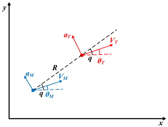
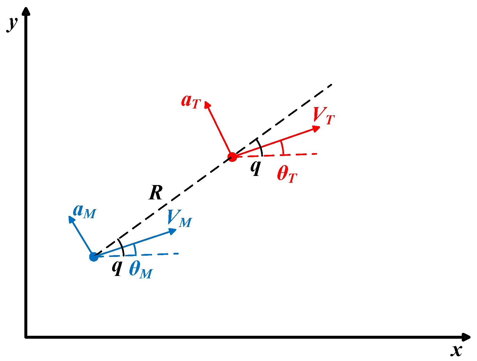
The geometrical relationship of the flight vehicle and target is illustrated in Figure 1. Here, the vehicle’s velocity, flight path angle, and normal acceleration are denoted as $V_M$, ${\theta }_M$, and $a_M$, while the target’s corresponding parameters are $V_T$, ${\theta }_T$, and $a_T$. R represents the relative distance between the flight vehicle and target and q denotes the line of sight (LOS) angle. According to [8], the relative kinematics model is formulated as

$$\begin{array}{c}\hfill \ddot{q}=-{\displaystyle \frac{2\dot{R}}{R}}\dot{q}+{\displaystyle \frac{a_{T}cos(q-{\theta }_T)}{R}}-{\displaystyle \frac{a_{M}cos(q-{\theta }_M)}{R}}\end{array}$$

(1)

Figure 1. Motion and geometrical relationship of the flight vehicle and target.

The planar flight vehicle dynamics are described by

$$\begin{array}{cc}\hfill & \dot{\alpha }={\displaystyle \frac{1}{m{V}_M}}(-L+mgcos{\theta }_M)+{\omega }_z\hfill \\ \hfill & J_z{\dot{\omega }}_z=M_{\alpha }\alpha +M_{{\delta }_z}{\delta }_z+M_{{\omega }_z}{\omega }_z\hfill \\ \hfill & a_M=-gcos{\theta }_M+{\displaystyle \frac{L}{m}}\hfill \\ \hfill & \dot{\vartheta }={\omega }_z,\alpha =\vartheta -{\theta }_M\hfill \end{array}$$

(2)

where $\alpha$, ${\delta }_z$, ${\omega }_z$, and $\vartheta$ are the angle of attack, rudder deflection for pitch control, pitch angular rate, and pitch angle, respectively, and $M_{\alpha },M_{{\omega }_z},M_{{\delta }_z}$ are their moment contributions. m represents the flight vehicle mass, g denotes the gravitational acceleration, $J_z$ is the pitch moment of inertia, and L stands for the lift force.

The expressions of $M_{\alpha }$, $M_{{\delta }_z}$, $M_{{\omega }_z}$, L are shown as $M_{\alpha }=57.3QSl{m}_z^{\alpha }$, $M_{{\delta }_z}=57.3QSl{m}_z^{{\delta }_z}$, $M_{{\omega }_z}={\displaystyle \frac{QS{l}^2{m}_z^{\omega z}}{V_M}},L=57.3QS{c}_y^{\alpha }\alpha$. The dynamic pressure, aerodynamic reference area, and reference length are denoted as Q, S, and l, respectively. $c_y^i,m_z^j$$(i=\alpha ,{\delta }_z;j=\alpha ,$ ${\omega }_z)$ represent nominal values of the aerodynamic coefficients. Defining $x_1=\dot{q}$, $x_2=\alpha$, $x_3={\omega }_z$, and $u={\delta }_z$, the state equations of the IGC model are given by

$$\begin{array}{cc}\hfill {\dot{x}}_1& =f_{x_1}+b_{x_1}{x}_2+d_1\hfill \\ \hfill {\dot{x}}_2& =f_{x_2}+x_3+d_2\hfill \\ \hfill {\dot{x}}_3& =f_{x_3}+b_{x_3}u+d_3\hfill \end{array}$$

(3)

The expressions of $f_{x1}$, $f_{x2}$, $f_{x3}$, $b_{x1}$, $b_{x3}$ and the lumped disturbances $d_1$, $d_2$, $d_3$ are given as

$$\begin{array}{cc}\hfill f_{x_1}& =-{\displaystyle \frac{2\dot{R}}{R}}\dot{q}+{\displaystyle \frac{gcos(q-{\theta }_M)}{R}}cos\left({\theta }_M\right)\hfill \\ \hfill f_{x_2}& ={\displaystyle \frac{-57.3QS{c}_y^{\alpha }\alpha }{m{V}_M}}\hfill \\ \hfill f_{x_3}& ={\displaystyle \frac{57.3QSl{m}_z^{\alpha }\alpha }{J_z}}+{\displaystyle \frac{QS{l}^2{m}_z^{{\omega }_z}{\omega }_z}{J_z{V}_M}}\hfill \\ \hfill b_{x_1}& ={\displaystyle \frac{-57.3QS{c}_y^{\alpha }cos(q-{\theta }_M)}{mR}}\hfill \\ \hfill b_{x_3}& ={\displaystyle \frac{57.3QSl{m}_z^{{\delta }_z}}{J_z}}\hfill \\ \hfill d_1& =d_1(c_y^{\alpha },{\Delta }_1)+{\displaystyle \frac{a_{T}cos(q-{\theta }_T)}{R}}\hfill \\ \hfill d_2& =d_2(c_y^{\alpha },{\Delta }_2)+{\displaystyle \frac{gcos\left({\theta }_M\right)}{V_M}}\hfill \\ \hfill d_3& =d_3(m_z^{\alpha },m_z^{{\omega }_z},m_z^{{\delta }_z},{\Delta }_3)\hfill \end{array}$$

(4)

where ${\Delta }_i(i=1,2,3)$ represent external disturbances acting on the flight vehicle and $d_i(i=1,2,3)$ denote lumped disturbances.

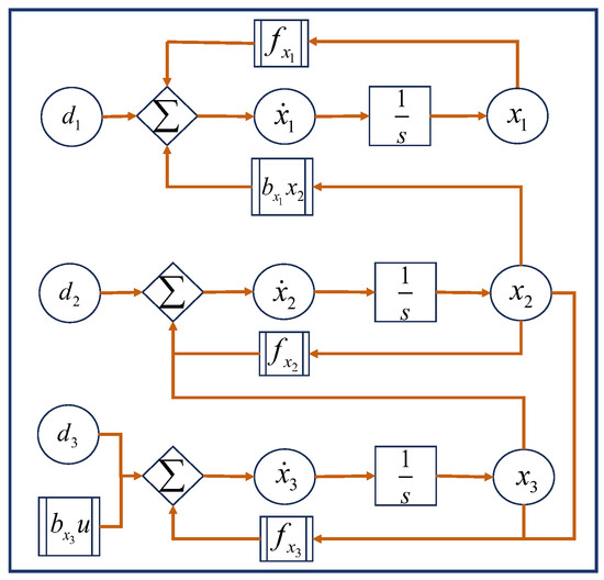
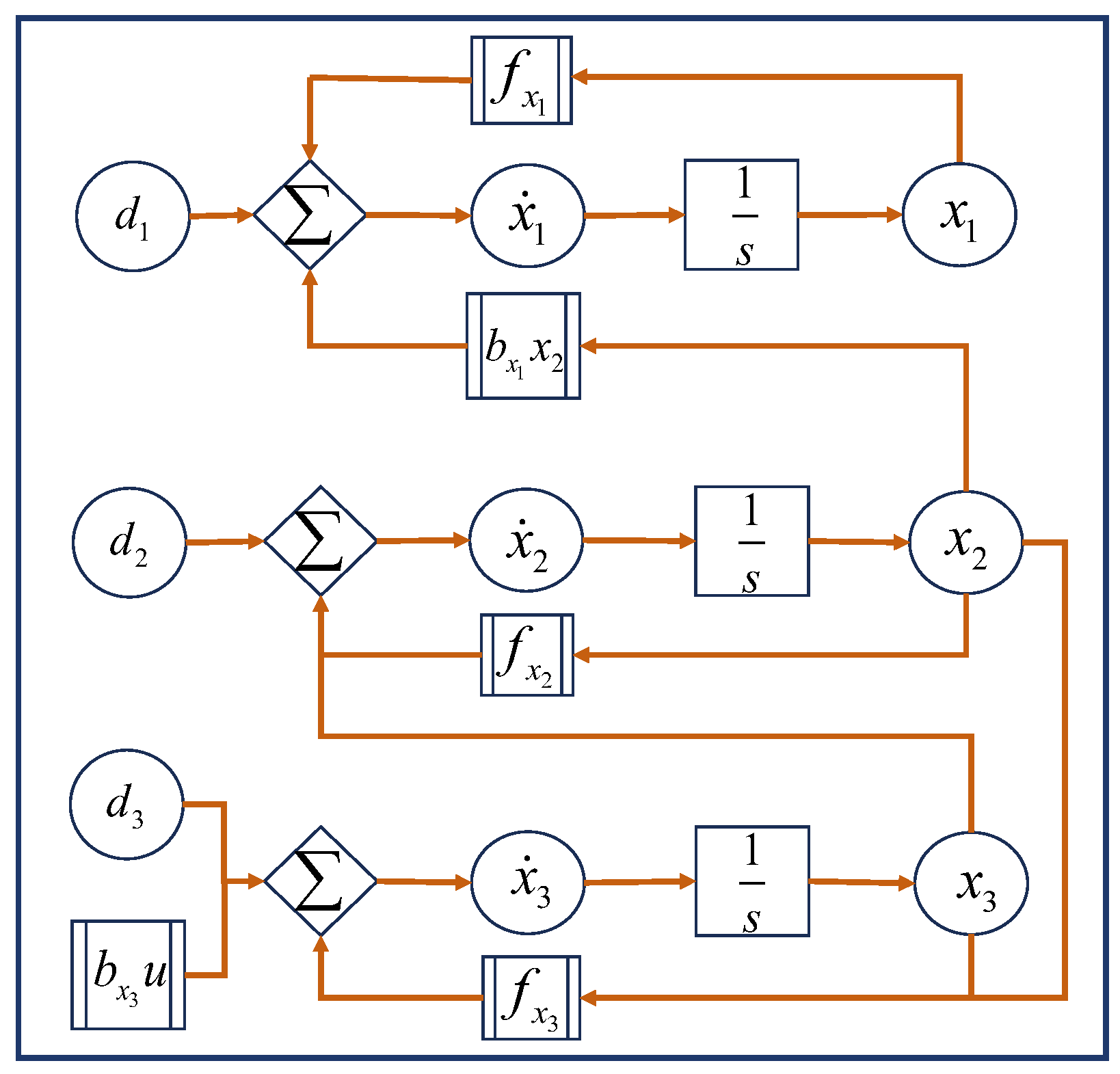
The block diagram of the IGC model is presented in Figure 2 to intuitively illustrate the dynamic relationships between state variables.

Figure 2. Block diagram of the IGC model.

Define $x_{1d}$, $x_{2d}$, and $x_{3d}$ as the desired signals for $x_1$, $x_2$, and $x_3$, respectively, and the error vector can be defined as $E=[e_1,e_2,e_3]=[x_1-x_{1d},x_2-x_{2d},x_3-x_{3d}]$. Here, $x_{1d}$ denotes the desired LOS angular rate and is set to zero to ensure a small terminal miss distance. Then, the error dynamic system can be formulated as

$$\begin{array}{cc}\hfill {\dot{e}}_1& =f_{x_1}+b_{x_1}{x}_{2c}+b_{x_1}{h}_2+b_{x_1}{e}_2+d_1\hfill \\ \hfill {\dot{e}}_2& =f_{x_2}+x_{3c}+h_3+e_3+d_2-{\dot{x}}_{2d}\hfill \\ \hfill {\dot{e}}_3& =f_{x_3}+b_{x_3}u+d_3-{\dot{x}}_{3d}\hfill \end{array}$$

(5)

where $x_{2d}$, $x_{3d}$ denote the outputs of the first-order low-pass filters with the inputs of the virtual control laws $x_{2c}$, $x_{3c}$, respectively. The output and input errors of the filters are defined by $h_2$ = $x_{2d}-x_{2c}$ and $h_3$ = $x_{3d}-x_{3c}$.

Remark 1.

Within the Dynamic Surface Control (DSC) framework, the strategic incorporation of first-order filters is a core design feature to avoid the “explosion of complexity” inherent in traditional backstepping [23,24]. The filtered outputs, $x_{2d}$ and $x_{3d}$, are not merely filtered signals but are explicitly assigned as the desired trajectories to be tracked. The redefinition transforms the original virtual control laws into smooth, realizable commands suitable for tracking. Thus, although derived via filtering, $x_{2d}$ and $x_{3d}$ are functionally assigned as the desired signals within the closed-loop architecture, justifying the standard error definitions $e_2=x_2-x_{2d}$ and $e_3=x_3-x_{3d}$.

Assumption 1 ([6]).

The lumped uncertainties $d_i(i=1,2,3)$ and their first-order derivatives are bounded, which satisfy $|d_i|\le {ϵ}_i,\left|{\dot{d}}_i\right|\le {\mu }_i(i=1,2,3)$, where ${\mu }_i$ and ${ϵ}_i$ are positive constants.

3. Analysis and Measurement of Influence on Convergence Rate for Flight Vehicles

In this section, the influence factors including model nonlinearities and couplings of the flight vehicle, which impose on the convergence, are analyzed by the Lyapunov stability theory. Then, based on the analysis, a convergence rate estimation mechanism is developed for the flight vehicle to further exploit and accelerate the convergence rate.

3.1. The Influence Factors on Convergence Rate of Interceptors

For simplicity in convergence rate analysis, the impact of the lumped disturbances and filter errors in Equation (5) are ignored temporally. The flight vehicle’s error states are, thus, rewritten as

$$\begin{array}{cc}\hfill {\dot{e}}_i& =F_i+S_i+G_i{x}_{(i+1)d},i=1,2\hfill \\ \hfill {\dot{e}}_3& =F_3+G_{3}u\hfill \end{array}$$

(6)

where $F_i=f_{x_i}-{\dot{x}}_{id}(i=1,2,3)$; $G_1=b_{x_1}$, $G_2=1$, $G_3=b_{x_3}$; $S_i=G_i{e}_{i+1}(i=1,2)$. $F_i$ and $S_i$ denote the model nonlinearities and couplings within the flight vehicle, respectively. Therein, $S_1$ represents the couplings between the guidance subsystem and the control subsystem, and $S_2$ denotes the couplings existing in the attitude control system of the flight vehicle. Thus, our main work in this part is to analyze how those influence factors (model nonlinearities and couplings) influence the convergence of the flight vehicle.

In backstepping control framework, the control laws can be designed as

$$\begin{array}{cc}\hfill x_{(i+1)d}& =-G_i^{-1}\left(F_i+S_i+\Theta \left(e_i\right)\right),i=1,2\hfill \\ \hfill u& =-G_3^{-1}\left(F_3+\Theta \left(e_3\right)\right)\hfill \end{array}$$

(7)

where $\Theta \left(e_i\right)$ is a function to be constructed that satisfies $e_i\Theta \left(e_i\right)\ge 0(i=1,2,3)$. Then, the Lyapunov function candidate is considered as

$$\begin{array}{cc}\hfill V& =\sum _{i=1}^3{\displaystyle \frac{1}{2}}{e}_i^2\hfill \end{array}$$

(8)

Together with (7), taking the derivative of Equation (8) yields

$$\begin{array}{c}\hfill {\dot{V}}_a=\sum _{i=1}^3{e}_i{\dot{e}}_i=-\sum _{i=1}^3{e}_i\Theta \left(e_i\right)\le 0\end{array}$$

(9)

where ${\dot{V}}_a$ denotes the derivative of V under the control laws (7). Note $e_i\Theta \left(e_i\right)\ge 0$, and by the Lyapunov stability theory, it can be concluded that the control laws in Equation (7) can ensure the stability of the error dynamic system (6) for the flight vehicle. However, the influence of the model nonlinearities $F_i(i=1,2,3)$ and the couplings $S_i(i=1,2)$ on the convergence of the flight vehicle are not analyzed, which are eliminated by the control laws (7).

Consequently, to perform the analysis of the influence factors on convergence rate, the control laws can be designed as

$$\begin{array}{cc}\hfill x_{(i+1)d}& =-G_i^{-1}\Theta \left(e_i\right),i=1,2,u=-G_3^{-1}\Theta \left(e_3\right)\hfill \end{array}$$

(10)

Then, taking the derivative of Equation (8) and combining with Equation (10), we can obtain

$$\begin{array}{c}\hfill {\dot{V}}_b=\sum _{i=1}^3{e}_i{\dot{e}}_i=-\sum _{i=1}^3{e}_i\Theta \left(e_i\right)+\sum _{i=1}^3{e}_i{F}_i+\sum _{i=1}^2{e}_i{S}_i\end{array}$$

(11)

where ${\dot{V}}_b$ represents the derivative of V under the control laws (10). Define $\Omega =\{S_i,F_i\}$, and consider one element in $\Omega$ with the other ignored temporarily. Therefore, for any element $\omega \in \Omega$, the influence on convergence rate can be divided into three cases: (i) for $e_i\omega <0$, ${\dot{V}}_b<{\dot{V}}_a<0$ holds and the flight vehicle system under the control laws (10) converges faster than that under the backstepping-based control laws (7); (ii) for $e_i\omega =0$, ${\dot{V}}_b={\dot{V}}_a<0$, which represents the convergence, is equally affected under the backstepping-based control laws (7) and the control laws (10); (iii) for $e_i\omega >0$, it can be observed that $\omega$ hinders the convergence of the flight vehicle system with ${\dot{V}}_a<{\dot{V}}_b<0$. The above analysis reveals the influence of model nonlinearities and coupling terms on the convergence of the flight vehicle system, and the convergence rate estimation mechanism for the flight vehicle system is developed to measure and leverage the influence to accelerate the convergence of the flight vehicle system.

3.2. Convergence Rate Estimation Mechanism for Flight Vehicles

First, a convergence rate indicator of the integrated guidance and control system is developed to measure the impact of the convergence rate affected by model nonlinearities and couplings within flight vehicles. Then, based on the developed indicator, the influence of those terms is explored, transformed, and utilized to accelerate the convergence of the flight vehicle’s guidance and control system. Furthermore, two lemmas are given to demonstrate the transformed influence of those terms on the convergence rate of the interceptor, and a quantitative relationship between those terms and the convergence rate is constructed.

The definition for the convergence rate indicator of the flight vehicle is introduced to better exploit the accelerated convergence characteristics of the flight vehicle’s internal factors.

Definition 1.

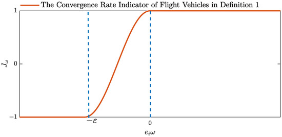
The convergence rate indicator for integrated guidance and control system is designed as

$$J_{\omega }=\left\{\begin{array}{cc}1\hfill & e_i\omega \in (0,\infty )\hfill \\ cos\left({\displaystyle \frac{1}{\epsilon }}\pi e_i\omega \right)\hfill & e_i\omega \in (-\epsilon ,0]\hfill \\ -1\hfill & e_i\omega \in (-\infty ,-\epsilon ),\hfill \end{array}\right.\psi =k_c\omega$$

(12)

where $\omega =F_i(i=1,2,3),S_i(i=1,2)$, $k_c>1$, and ε is a small coefficient with $\epsilon >0$.

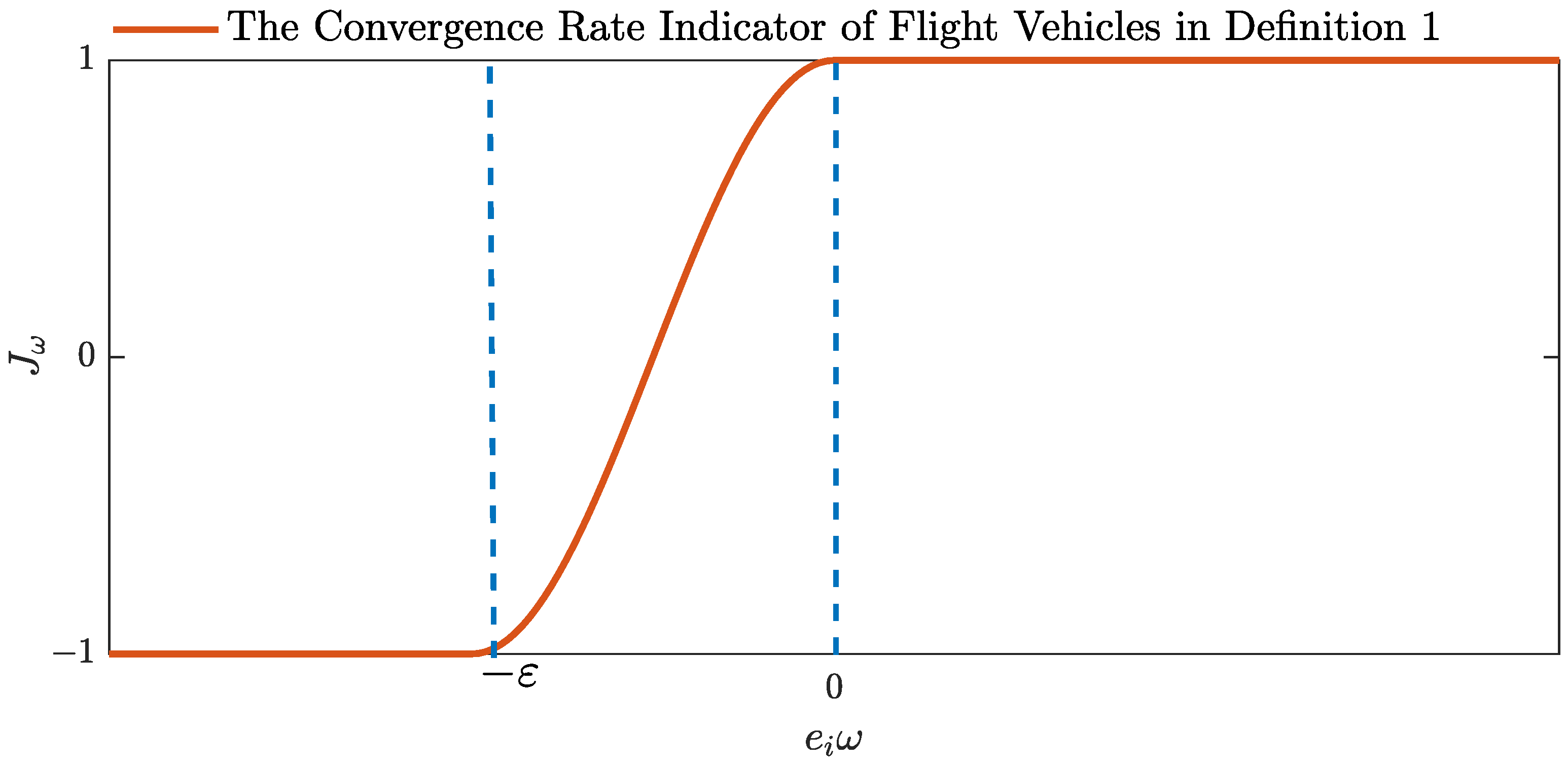
The convergence rate indicator in Definition 1 employs a cosine function during $e_i\omega \in (-\epsilon ,0]$ to sacrifice partial utilization of convergence characteristics for chattering mitigation, while the small coefficient $k_c$ not only amplifies beneficial convergence characteristics but also transforms and utilizes detrimental convergence characteristics. The indicator function in Definition 1 is shown in Figure 3.

Figure 3. Indicator in Definition 1.

Then, the following Lemma is given to demonstrate the transformed influence of nonlinearities and coupling terms on the convergence of the flight vehicle system, and stability analysis framework is established.

Lemma 1.

The convergence rate indicator of flight vehicles is designed in Definition 1, then, the following inequality holds:

$$\begin{array}{c}\hfill e_i\omega -e_i{J}_{\omega }\psi \le 0\end{array}$$

(13)

Proof. 

For brevity, we define $Y=e_i\omega -e_i{J}_{\omega }\psi$. Considering the sign of $e_i\omega$, three cases require analysis: (i) If $e_i\omega \in (0,\infty )$, $Y=e_i\omega (1-k_c)<0$ is satisfied with $J_{\omega }=1$. (ii) On the condition $e_i\omega \in (-\epsilon ,0]$, $Y=e_i\omega \left(1-k_{c}cos({\displaystyle \frac{1}{\epsilon }}\pi e_i\omega )\right)<0$ holds with $J_{\omega }=cos\left({\displaystyle \frac{1}{\epsilon }}\pi e_i\omega \right)$. (iii) For $e_i\omega \in (-\infty ,-\epsilon )$, it is explicit to find $Y=e_i\omega (1+k_c)<0$ with $J_{\omega }=-1$. In summary, we can obtain $Y\le 0$. The proof for Lemma 1 is completed.    □

Essentially, Equation (13) embodies a modification to the derivative of the Lyapunov function and the adjustment is instrumental in leveraging Lemma 1 to simplify both the control laws’ design and the stability analysis. Based on the convergence rate indicator in Definition 1, the accelerated convergence characteristics of nonlinearities and coupling terms are injected into the following control laws:

$$\begin{array}{cc}\hfill x_{(i+1)d}& =-G_i^{-1}\left(J_{F_i}{k}_c{F}_i+J_{S_i}{k}_c{S}_i+\Theta \left(e_i\right)\right),i=1,2\hfill \\ \hfill u& =-G_3^{-1}\left(J_{F_3}{k}_c{F}_3+\Theta \left(e_3\right)\right)\hfill \end{array}$$

(14)

Different from the backstepping-based control laws (7) which directly estimates and compensates model nonlinearities $F_i(i=1,2,3)$ and coupling terms $S_i(i=1,2)$, the convergence rate indicator actively incorporates their influence into the novel control laws (14) to accelerate convergence and further improve control performance. Furthermore, the convergence rate indicator in Definition 1 augments beneficial convergence characteristics, transforms detrimental convergence characteristics to be utilized, and alleviates the high-frequency chattering phenomena.

To construct the quantitative relationship between the influence factors (model nonlinearities, coupling terms) and convergence rate, Assumption 2 and Lemma 2 are proposed.

Assumption 2

([25]). For the model nonlinearities $F_i$ and coupling terms $S_i$, there exist continuous non-negative functions $W_{F_i}\left(t\right)\ge 0(i=1,2,3)$ and $W_{S_i}\left(t\right)\ge 0(i=1,2)$, satisfying

$$\begin{array}{c}\hfill |F_i|\ge W_{F_i}\left(t\right)|e_i|,|S_i|\ge W_{S_i}\left(t\right)\left|e_i\right|\end{array}$$

(15)

where the equalities hold if and only if $F_i=0,S_i=0.$

Remark 2.

The physical implication of Assumption 2 is that it quantitatively describes the bounding influence of the system nonlinearities $F_i$ and coupling effects $S_i$ on the dynamics of the tracking error $e_i$. The inequalities in (15) indicate that the magnitudes of $F_i$ and $S_i$ grow at least at a rate proportional to the error $e_i$. This is reasonable in practical flight vehicle dynamics. For instance, aerodynamic force/moment nonlinearities ($F_i$) and the couplings within the guidance subsystem and the control subsystem ($S_i$) typically have an intensity correlated with the deviation in system states, and these state deviations are ultimately reflected in $e_i$. Regarding the applicability, Assumption 2 requires that the system’s nonlinearities and the couplings are structured, which is met in most well-designed flight vehicle models. The existence of the functions $W_{F_i}\left(t\right)$ and $W_{S_i}\left(t\right)$ provides the mathematical foundation for quantifying the impact of these dynamic effects in the subsequent convergence rate analysis.

Lemma 2.

The IGC system of the flight vehicle under the indicator-based control laws (14) has a faster convergence rate than the backstepping-based control laws (7).

Proof. 

For the error dynamic system (6), the derivative of V under the control laws (8) can be written as ${\dot{V}}_c={\sum }_{i=1}^3{\dot{V}}_{c_i}$, where

$$\begin{array}{c}\hfill {\dot{V}}_{c_i}=e_i{\dot{e}}_i=A_i+B_i-e_i\Theta \left(e_i\right),i=1,2,3\end{array}$$

(16)

with $A_i=(1-J_{F_i}{k}_c)F_i{e}_i(i=1,2,3)$, $B_i=(1-J_{S_i}{k}_c)S_i{e}_i(i=1,2)$, $B_3=0$. According to Assumption 2 and Lemma 1, the following inequalities hold

$$\begin{array}{cc}\hfill A_i& =(1-J_{F_i}{k}_c)F_i{e}_i\le -|1-J_{F_i}{k}_c|W_{F_i}\left(t\right)e_i^2\hfill \end{array}$$

(17)

$$\begin{array}{cc}\hfill B_i& =(1-J_{S_i}{k}_c)S_i{e}_i\le -|1-J_{S_i}{k}_c|W_{S_i}\left(t\right)e_i^2\hfill \end{array}$$

(18)

Substituting Equations (17) and (18) into Equation (16) yields

$$\begin{array}{cc}\hfill {\dot{V}}_{c_i}& =A_i+B_i-e_i\Theta \left(e_i\right)\hfill \\ \hfill & \le -|1-J_{F_i}{k}_c|W_{F_i}\left(t\right)e_i^2-|1-J_{S_i}{k}_c|W_{S_i}\left(t\right)e_i^2-e_i\Theta \left(e_i\right)\hfill \end{array}$$

(19)

where $\Theta \left(e_i\right)$ is a function to be constructed that satisfies $e_i\Theta \left(e_i\right)\ge 0$. For simplicity, $\Theta \left(e_i\right)$ can be defined as $\Theta \left(e_i\right)=k_i{e}_i$ and $k_i\ge 0$. Thus, it follows

$$\begin{array}{c}\hfill {\dot{V}}_{c_i}\le -{\displaystyle \frac{1}{2}}{\beta }_{1,i}{e}_i^2=-{\beta }_{1,i}{V}_{c_i}\le 0\end{array}$$

(20)

where ${\beta }_{1,i}=2(k_i+|1-J_{F_i}{k}_c|W_{F_i}\left(t\right)+|1-J_{S_i}{k}_c|W_{S_i}\left(t\right))$, and ${\dot{V}}_{c_i}=-{\displaystyle \frac{1}{2}}{\beta }_{1,i}{e}_i^2$ holds only when $F_i=0$, $S_i=0$.

Then, by the comparison principle [26], it is easy to obtain the following inequalities

$$\begin{array}{c}\hfill V_{c_i}\left(t\right)\le V_{c_i}\left(0\right)e^{-{\beta }_{1,i}t},|e_i\left(t\right)|\le |e_i\left(0\right)|e^{-\frac{1}{2}{\beta }_{1,i}t}\end{array}$$

(21)

where ${\displaystyle \frac{{\beta }_{1,i}}{2}}=k_i+|1-J_{F_i}{k}_c|W_{F_i}\left(t\right)+|1-J_{S_i}{k}_c|W_{S_i}\left(t\right)$ is the convergence rate under the indicator-based control laws (14).

Similarly, for the backstepping-based control laws (7), $V_{a_i}\left(t\right)$ and $e_i\left(t\right)$ can be derived as

$$\begin{array}{c}\hfill V_{a_i}\left(t\right)=V_{a_i}\left(0\right)e^{-{\beta }_{2,i}t},|e_i\left(t\right)|= |e_i\left(0\right)|e^{-\frac{1}{2}{\beta }_{2,i}t}\end{array}$$

(22)

where ${\displaystyle \frac{{\beta }_{2,i}}{2}}=k_i$ is the convergence rate for the backstepping control method.

By comparing the convergence rates ${\beta }_{1,i}$ and ${\beta }_{2,i}(i=1,2,3)$ in Equations (21) and (22), it follows ${\beta }_{2,i}\le {\beta }_{1,i}$, and we can obtain that the IGC system governed by the indicator-based control laws (14) can converge faster compared to the system controlled under backstepping control laws (7).    □

Remark 3.

The expression for the convergence rate ${\displaystyle \frac{{\beta }_{1,i}}{2}}$ shows that it consists of a fixed gain $k_i$ and the time-varying terms $|1-J_{F_i}{k}_c|W_{F_i}\left(t\right)$ and $|1-J_{S_i}{k}_c|W_{S_i}\left(t\right)$. According to Assumption 2, whenever the system nonlinearities $F_i$ or coupling terms $S_i$ are non-zero, the time-varying terms $W_{F_i}\left(t\right)$ and $W_{S_i}\left(t\right)$ are positive. This implies that the proposed indicator-based control law actively leverages the intrinsic system dynamics, resulting in a non-negative increment $\Delta {\beta }_i\left(t\right)/2$ in the instantaneous convergence rate compared to the traditional backstepping convergence rate ${\displaystyle \frac{{\beta }_{2,i}}{2}}=k_i$. This increment is defined as $\Delta {\beta }_i\left(t\right)/2=|1-J_{F_i}{k}_c|W_{F_i}\left(t\right)+|1-J_{S_i}{k}_c|W_{S_i}\left(t\right)\ge 0$. Consequently, the relationship between the conventional and proposed convergence rates can be formulated as ${\beta }_{1,i}={\beta }_{2,i}+\Delta {\beta }_i\left(t\right)$. This formulation shows that the superior convergence performance of the proposed method stems from strategically exploiting the influence of the model nonlinearities and coupling terms.

Lemma 2 exploits the influence of model nonlinearities and coupling terms based on the convergence rate indicator to accelerate the convergence of the IGC system, and the value of convergence rate under traditional backstepping control laws and the indicator-based control laws are given, respectively, to verify the accelerated convergence effect of the proposed method from the theoretical perspective. In the next section, the convergence rate estimation mechanism is utilized to design the fast robust IGC laws for the flight vehicles under the lumped uncertainties $d_i(i=1,2,3)$.

4. Fast Robust IGC Scheme

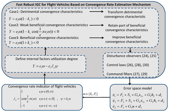
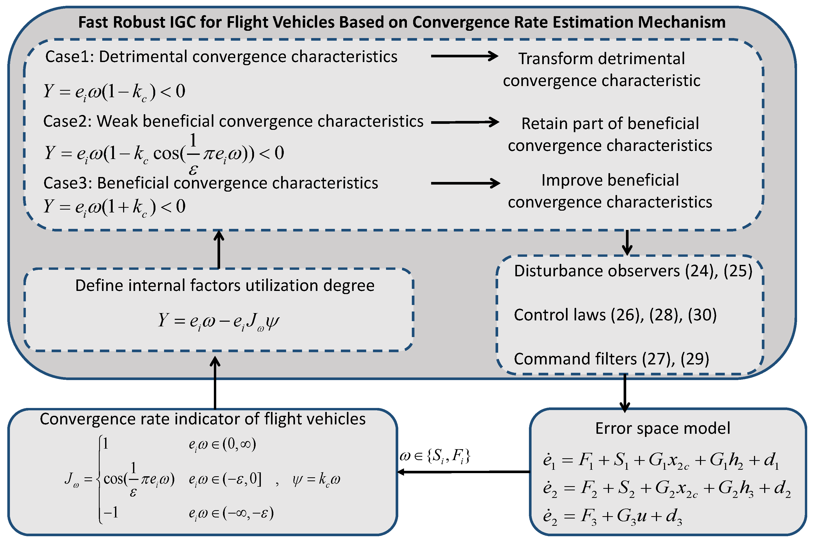
In this section, a fast robust IGC approach is designed based on the convergence rate estimation mechanism to accelerate the convergence of the IGC system. The unmatched lumped uncertainties in the flight vehicle system are addressed via disturbance observers and backstepping control. In addition, the first-order filtering is employed to address the computational explosion problem existing in the backstepping control framework. The stability analysis of the closed-loop system is performed. The schematic diagram of the proposed control scheme is demonstrated in Figure 4.

Figure 4. Schematic diagram of the proposed IGC scheme.

4.1. Indicator-Based Robust IGC Law Design

Due to model uncertainties and external disturbances in the flight vehicle system, an effective disturbance observer is designed to improve the robustness of the control system. Considering the following system

$$\begin{array}{cc}\hfill {\dot{e}}_i& =F_i+S_i+G_i{x}_{(i+1)c}+G_i{h}_{i+1}+d_i,i=1,2\hfill \\ \hfill {\dot{e}}_3& =F_3+G_{3}u+d_3\hfill \end{array}$$

(23)

where $x_{(i+1)d}(i=1,2)$ denote the outputs of the first-order low-pass filters with the inputs of the virtual control laws $x_{(i+1)c}$, and $d_i(i=1,2,3)$ denote the lumped disturbances. The output and input errors of the filters are defined as $h_{i+1}=x_{(i+1)d}-x_{(i+1)c}$.

The finite-time convergence disturbance observer [27] is introduced as follows:

$$\begin{array}{cc}\hfill {\dot{\widehat{e}}}_i& =F_i+S_i+G_i{x}_{(i+1)c}+G_i{h}_{i+1}+\widehat{d_i}\hfill \\ \hfill {\dot{\widehat{d}}}_i& =-l_{i1}^2\left(l_{i2}\arctan ({\widehat{e}}_i-e_i)+l_{i3}\arctan ({\displaystyle \frac{1}{l_{i1}}}\widehat{d_i})\right),i=1,2\hfill \end{array}$$

(24)

$$\begin{array}{cc}\hfill {\dot{\widehat{e}}}_3& =F_3+G_{3}u+{\widehat{d}}_3\hfill \\ \hfill {\dot{\widehat{d}}}_3& =-l_{31}^2\left(l_{32}\arctan ({\widehat{e}}_3-e_3)+l_{33}\arctan ({\displaystyle \frac{1}{l_{31}}}{\widehat{d}}_3)\right)\hfill \end{array}$$

(25)

where $\widehat{d_i}$ and ${\widehat{e}}_i$ are the estimates of $d_i$ and $e_i(i=1,2,3)$. $l_{i1}$, $l_{i2}$, and $l_{i3}(i=1,2,3)$ are positive constants to be designed.

Under Assumption 1, the parameters $l_{i1}$, $l_{i2}$, and $l_{i3}$ can be systematically tuned to ensure precise estimation of $d_i$ achieving $|{\widehat{d}}_i-d_i|=0$ as $t\to \infty$. Subsequently, the control scheme for the IGC system is designed using the following procedure.

Step 1: Based on the convergence rate indicator in Definition 1 and the proposed disturbance observers (24) and (25), the virtual control law incorporating the influence of nonlinearities and coupling terms in the first equation of system (5) is designed as

$$\begin{array}{c}\hfill x_{2c}=-G_1^{-1}(J_{S_1}{k}_c{S}_1+J_{F_1}{k}_c{F}_1+{\widehat{d}}_1+k_1{e}_1)\end{array}$$

(26)

Step 2: The first-order filter is given to obtain ${\dot{x}}_{2d}$:

$$\begin{array}{c}\hfill {\tau }_1{\dot{x}}_{2d}+x_{2d}=x_{2c},x_{2c}\left(0\right)=x_{2d}\left(0\right)\end{array}$$

(27)

where ${\tau }_1$ is a positive constant to be designed.

Step 3: As for the second equation of system (5), the virtual control law is designed combining with the first-order filter value ${\dot{x}}_{2d}$ in Step 2:

$$\begin{array}{c}\hfill x_{3c}=-\left(J_{S_2}{k}_c{S}_2+J_{F_2}{k}_c{F}_2+{\widehat{d}}_2+k_2{e}_2\right)\end{array}$$

(28)

Step 4: Similar to Step 2, ${\dot{x}}_{3d}$ can be obtained:

$$\begin{array}{c}\hfill {\tau }_2{\dot{x}}_{3d}+x_{3d}=x_{3c},x_{3c}\left(0\right)=x_{3d}\left(0\right)\end{array}$$

(29)

where ${\tau }_2>0$ is a time constant.

Step 5: The proposed control law is designed as

$$\begin{array}{c}\hfill u=-G_3^{-1}\left(J_{F_3}{k}_c{F}_3+{\widehat{d}}_3+k_3{e}_3\right)\end{array}$$

(30)

Remark 4.

The method proposed in [25] was originally developed for robotic systems with moderate real-time constraints and, thus, cannot be directly applied to flight vehicle systems that demand strict real-time performance. To meet the specific requirements of flight vehicle systems, the paper proposes a fast robust IGC method incorporating the finite-time convergence disturbance observer and a specially designed convergence rate estimation mechanism for flight vehicles, which ensures real-time and rapid response requirements under strong time-varying uncertainties. Moreover, the proposed method considers the model nonlinearities of the flight vehicle, which are analyzed and utilized to improve the control performance of the flight vehicle systems. However, the model nonlinearities are not taken into account in [6], and thus, the control performance of the proposed method outperforms that in [6], of which the conclusions are verified by the simulation results in Section 5.

The overall implementation procedure of the proposed fast robust IGC scheme is summarized in Algorithm 1, which provides a step-by-step computational framework for practical implementation.

Algorithm 1 A fast robust integrated guidance and control scheme for flight vehicles based on convergence rate estimation mechanism

Require: System parameters: $V_m$, $V_t$, g, $R_0$, $q_0$, etc.; Controller gains: $k_1$, $k_2$, $k_3$, ${\tau }_1$, ${\tau }_2$, $k_c$;     Simulation settings: h Ensure: System states: $\mathbf{X}$; Control history: u     Initialization:     Set initial states $\mathbf{X}\left(0\right)$ and errors $e_1$, $e_2$, $e_3$     Initialize disturbance observers: ${\widehat{d}}_1$, ${\widehat{d}}_2$, ${\widehat{d}}_3\leftarrow 0$     Initialize filters: $x_{2d}\left(0\right)\leftarrow 0.3238$, $x_{3d}\left(0\right)\leftarrow 1.2948$     $t\leftarrow 0$     Main Simulation Loop:     while  $t\le t_f$  do      1. State Update:      $\mathbf{X}\leftarrow \mathrm{RungeKutta}4(\mathrm{DynamicEquation},t,h,\mathbf{X})$      2. Update Tracking Errors:      $e_1\leftarrow x_1-x_{1d}$, $e_2\leftarrow x_2-x_{2d}$, $e_3\leftarrow x_3-x_{3d}$      3. Disturbance Observer Update:      ${\widehat{d}}_i\leftarrow {\widehat{d}}_i-l_{i1}^2[l_{i2}arctan({\widehat{e}}_i-e_i)+l_{i3}arctan({\widehat{d}}_i/l_{i1})],i=1,2,3$      4. Convergence Rate Estimation:        Compute indicators $J_{F_i}$, $J_{S_i}$ based on $e_i{F}_i$ and $e_i{S}_i$      5. Control Law Calculation:      $x_{2c}\leftarrow -G_1^{-1}(J_{S_1}{k}_c{S}_1+J_{F_1}{k}_c{F}_1+{\widehat{d}}_1+k_1{e}_1)$      $x_{3c}\leftarrow -(J_{S_2}{k}_c{S}_2+J_{F_2}{k}_c{F}_2+{\widehat{d}}_2+k_2{e}_2)$      $u\leftarrow -G_3^{-1}(J_{F_3}{k}_c{F}_3+{\widehat{d}}_3+k_3{e}_3)$      6. Control Saturation:      $u\leftarrow max(-{20}^{°},min({20}^{°},u))$      7. Filter Update:      ${\dot{x}}_{2d}\leftarrow (x_{2c}-x_{2d})/{\tau }_1$      ${\dot{x}}_{3d}\leftarrow (x_{3c}-x_{3d})/{\tau }_2$      if $\dot{R}>0$ then       break      end if      $t\leftarrow t+h$     end while     Output: Time histories of states, controls

4.2. Stability Analysis

Theorem 1.

For the guidance and control system (23), the control laws (26), (28), and (30) with the convergence rate indicator (12), disturbance observers (24) and (25) can ensure that the attitude angle errors of the closed-loop system are ultimately bounded.

Proof. 

The estimation errors of the disturbance observers are defined as ${\tilde{d}}_i={\widehat{d}}_i-d_i(i=1,2,3)$, where ${\widehat{d}}_i$ and $d_i$ denote the estimated disturbances and the true disturbances, respectively. According to Reference [28], there exist small positive constants ${\overline{d}}_i(i=1,2,3)$ satisfying $|{\tilde{d}}_i|<{\overline{d}}_i$. Substituting Equations (26), (28), and (30) into System (23), we can obtain

$$\begin{array}{cc}\hfill {\dot{e}}_1& =(1-J_{F_1}{k}_c)F_1+(1-J_{S_1}{k}_c)S_1+G_1{h}_2-{\tilde{d}}_1-k_1{e}_1\hfill \\ \hfill {\dot{e}}_2& =(1-J_{F_2}{k}_c)F_2+(1-J_{S_2}{k}_c)S_2+h_3-{\tilde{d}}_2-k_2{e}_2\hfill \\ \hfill {\dot{e}}_3& =(1-J_{F_3}{k}_c)F_3-{\tilde{d}}_3-k_3{e}_3\hfill \end{array}$$

(31)

The Lyapunov candidate function is considered as $V=V_1+V_2={\sum }_{i=1}^3{\displaystyle \frac{1}{2}}{e}_i^2+{\sum }_{i=2}^3{\displaystyle \frac{1}{2}}{h}_i^2$, and the derivative of V can be rewritten as

$$\begin{array}{c}\hfill \dot{V}=\underset{{\dot{V}}_1}{\underbrace{\sum _{i=1}^3{e}_i{\dot{e}}_i}}+\underset{{\dot{V}}_2}{\underbrace{\sum _{i=2}^3{h}_i{\dot{h}}_i}}\end{array}$$

(32)

Together with Equation (31) and the proved conclusion $e_i\omega -e_i{J}_{\omega }\psi \le 0$ in Lemma 1, ${\dot{V}}_1$ can be derived as

$$\begin{array}{cc}\hfill {\dot{V}}_1& =\underset{\le 0}{\underbrace{(1-J_{F_1}{k}_c)F_1{e}_1}}+\underset{\le 0}{\underbrace{(1-J_{S_1}{k}_c)S_1{e}_1}}+\underset{\le 0}{\underbrace{(1-J_{F_2}{k}_c)F_2{e}_2}}+\underset{\le 0}{\underbrace{(1-J_{S_2}{k}_c)S_2{e}_2}}+\underset{\le 0}{\underbrace{(1-J_{F_3}{k}_c)F_3{e}_3}}\hfill \\ & +G_1{h}_2{e}_1-{\tilde{d}}_1{e}_1-k_1{e}_1^2+h_3{e}_2-{\tilde{d}}_2{e}_2-k_2{e}_2^2-{\tilde{d}}_3{e}_3-k_3{e}_3^2\hfill \\ \hfill & \le G_1{h}_2{e}_1+{\overline{d}}_1|e_1|-k_1{e}_1^2+h_3{e}_2+{\overline{d}}_2|e_2|-k_2{e}_2^2+{\overline{d}}_3\left|e_3\right|-k_3{e}_3^2\hfill \\ \hfill & \le ({\displaystyle \frac{1}{12}}-k_1)e_1^2+({\displaystyle \frac{1}{2}}-k_2)e_2^2+({\displaystyle \frac{1}{4}}-k_3)e_3^2+6G_1^2{h}_2^2+h_3^2+6{\overline{d}}_1^2+{\overline{d}}_2^2+{\overline{d}}_3^2\hfill \end{array}$$

(33)

Combining with the filters (27) and (29), and assuming that ${\sigma }_{x_{2c}},{\sigma }_{x_{3c}}>0$ are the upper bounds of $\left|{\dot{x}}_{2c}\right|$, $\left|{\dot{x}}_{3c}\right|$, respectively, [20], ${\dot{V}}_2$ can be rewritten as

$$\begin{array}{cc}\hfill {\dot{V}}_2& =-{\displaystyle \frac{1}{{\tau }_1}}{h}_2^2-h_2{\dot{x}}_{2c}-{\displaystyle \frac{1}{{\tau }_2}}{h}_3^2-h_3{\dot{x}}_{3c}\hfill \\ \hfill & \le -({\displaystyle \frac{1}{{\tau }_1}}-1)h_2^2-({\displaystyle \frac{1}{{\tau }_2}}-1)h_3^2+{\displaystyle \frac{1}{4}}({\sigma }_{x_{2c}}^2+{\sigma }_{x_{3c}}^2)\hfill \end{array}$$

(34)

Subsequently, incorporating Equations (33) and (34) yields

$$\begin{array}{cc}\hfill \dot{V}& \le ({\displaystyle \frac{1}{12}}-k_1)e_1^2+({\displaystyle \frac{1}{2}}-k_2)e_2^2+({\displaystyle \frac{1}{4}}-k_3)e_3^2+(2-{\displaystyle \frac{1}{{\tau }_2}})h_3^2\hfill \\ \hfill & +6{\overline{d}}_1^2+{\overline{d}}_2^2+{\overline{d}}_3^2+{\displaystyle \frac{1}{4}}({\sigma }_{x_{2c}}^2+{\sigma }_{x_{3c}}^2)+(6G_1^2+1-{\displaystyle \frac{1}{{\tau }_1}})h_2^2\hfill \\ \hfill & =-2\lambda V+ϵ\hfill \end{array}$$

(35)

where $\lambda =\min \{k_1-{\displaystyle \frac{1}{12}},k_2-{\displaystyle \frac{1}{2}},k_3-{\displaystyle \frac{1}{4}},{\displaystyle \frac{1}{{\tau }_1}}-6G_1^2-1,{\displaystyle \frac{1}{{\tau }_2}}-2\}$, $ϵ=6{\overline{d}}_1^2+{\overline{d}}_2^2+{\overline{d}}_3^2+{\displaystyle \frac{1}{4}}({\sigma }_{x_{2c}}^2+{\sigma }_{x_{3c}}^2)$ with $k_1\ge {\displaystyle \frac{1}{12}}$, $k_2\ge {\displaystyle \frac{1}{2}}$, $k_3\ge {\displaystyle \frac{1}{4}}$, ${\displaystyle \frac{1}{{\tau }_1}}\ge 6G_1^2+1$, ${\displaystyle \frac{1}{{\tau }_2}}\ge 2$. Thus, according to [19], the attitude angle errors for the closed-loop system can converge to the domain concerning $\Omega =\{V|V\le {\displaystyle \frac{ϵ}{2\lambda }}\}$. Then, the closed-loop system of the flight vehicle is ultimately bounded. □

5. Simulation Studies

In this section, extensive numerical simulations are performed to verify the effectiveness and interception performance of the proposed fast robust method under lumped disturbances. The engagement scenario is initialized with the following parameters: the relative distance between the flight vehicle and target is $10 \mathrm{km}$; the initial flight path angle and constant velocity for the flight vehicle and target are ${45}^{°}$, ${120}^{°}$, $500\mathrm{m}/\mathrm{s}$, $250\mathrm{m}/\mathrm{s}$, respectively; the initial LOS angle is $q_0={30}^{°}$. The initial conditions of states and the control parameters for numerical simulations are given in Table 1.

Table 1. Simulation conditions and parameters.

Initial Conditions	All States	$\dot{\mathit{q}}\left(0\right)=0^{°}/\mathbf{s},\mathit{\alpha }\left(0\right)=0^{°},{\mathit{\omega }}_{\mathit{z}}\left(0\right)=0^{°}/\mathbf{s}$
Disturbance observers	Equation (24)   $(i=1)$	$l_{11}=1,l_{12}=5,l_{13}=4$
	Equation (24)   $(i=2)$	$l_{21}=1,l_{22}=5,l_{23}=4$
	Equation (24)   $(i=3)$	$l_{31}=1,l_{32}=5,l_{33}=4$
Control Parameters	Proposed Method	$k_1=0.1,k_2=2,k_3=5$
		${\tau }_1=0.2,{\tau }_2=0.1,\epsilon =0.001,k_c=1.1$
	RBC [10]	$k_1=0.1,k_2=2,k_3=5$
	SSMC [19]	$k_1=0.1,m=0.001,n=0.0001$
	CEUT [6]	$k_1=0.1,k_2=2,k_3=5$
		${\tau }_1=0.2,{\tau }_2=0.1,\epsilon =3\times {10}^{-4},k_c=0.1$

The aerodynamic parameters for the flight vehicle are given as ${\displaystyle \frac{57.3QS{C}_y^{\alpha }}{m{V}_M}}=0.3487$, ${\displaystyle \frac{57.3QS{C}_y^{{\delta }_z}}{m{V}_M}}=0.068$, ${\displaystyle \frac{57.3QSl{m}_z^{\alpha }}{J_z}}=-17.801$, ${\displaystyle \frac{QS{l}^2{m}_z^{{\omega }_z}}{J_z{V}_M}}=-0.2741$, ${\displaystyle \frac{57.3QSl{m}_z^{{\delta }_z}}{J_z}}=-31.267$. The constraints imposed on the actuator of the flight vehicle are given as $|{\delta }_z|\le {20}^{°},\left|{\dot{\delta }}_z\right|\le {200}^{°}/\mathrm{s}$. To systematically evaluate the interception performance of the proposed method, three representative cases are analyzed through comparative simulations against coupling effect utilization and transformation method (CEUT) [6], robust backstepping control (RBC) [10], and super-twisting sliding mode control (SSMC) [19]. For a fair comparison, the proposed method and the three benchmark methods are performed under the same engagement conditions and actuator constraints, using the same engineering criteria and identical control parameter sets. Note that the superior performance of the proposed method stems from transforming and utilizing the influence of model nonlinearities and coupling terms on convergence rate rather than from tuning parameters aimed specifically at accelerating convergence.

Remark 5.

The proposed method involves several design parameters, whose selections entail practical trade-offs. The parameters $k_i(i=1,2,3)$ directly influence the convergence rate: larger values generally yield faster convergence but may increase control effort and the risk of actuator saturation. The parameter ε, associated with the convergence rate indicator, regulates the transition smoothness near $e_i\omega =0$. A smaller ε can sharpen the response but may induce chattering, whereas a larger ε suppresses chattering at the potential cost of convergence performance. The gain $k_c$ enhances the convergence speed by actively utilizing nonlinearities and coupling effects. However, an excessively large $k_c$ will burden the control input. In practice, these parameters should be tuned to balance convergence speed, control effort, and chattering suppression, aligning with specific actuator limits and performance requirements.

Case 1: Additive disturbances $d_2=0.5sin\left(t\right)\mathrm{rad}$, $d_3=0.5sin\left(t\right)\mathrm{rad}/\mathrm{s}$ are added to the system of the flight vehicle with the target maneuver $a_T=30sin\left(0.25t\right){\mathrm{m}/\mathrm{s}}^2$. Meanwhile, it is assumed that the coefficients of aerodynamic forces and moments are added with an increasement, 20% of their nominal values, simultaneously.

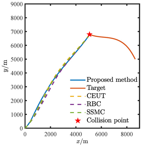
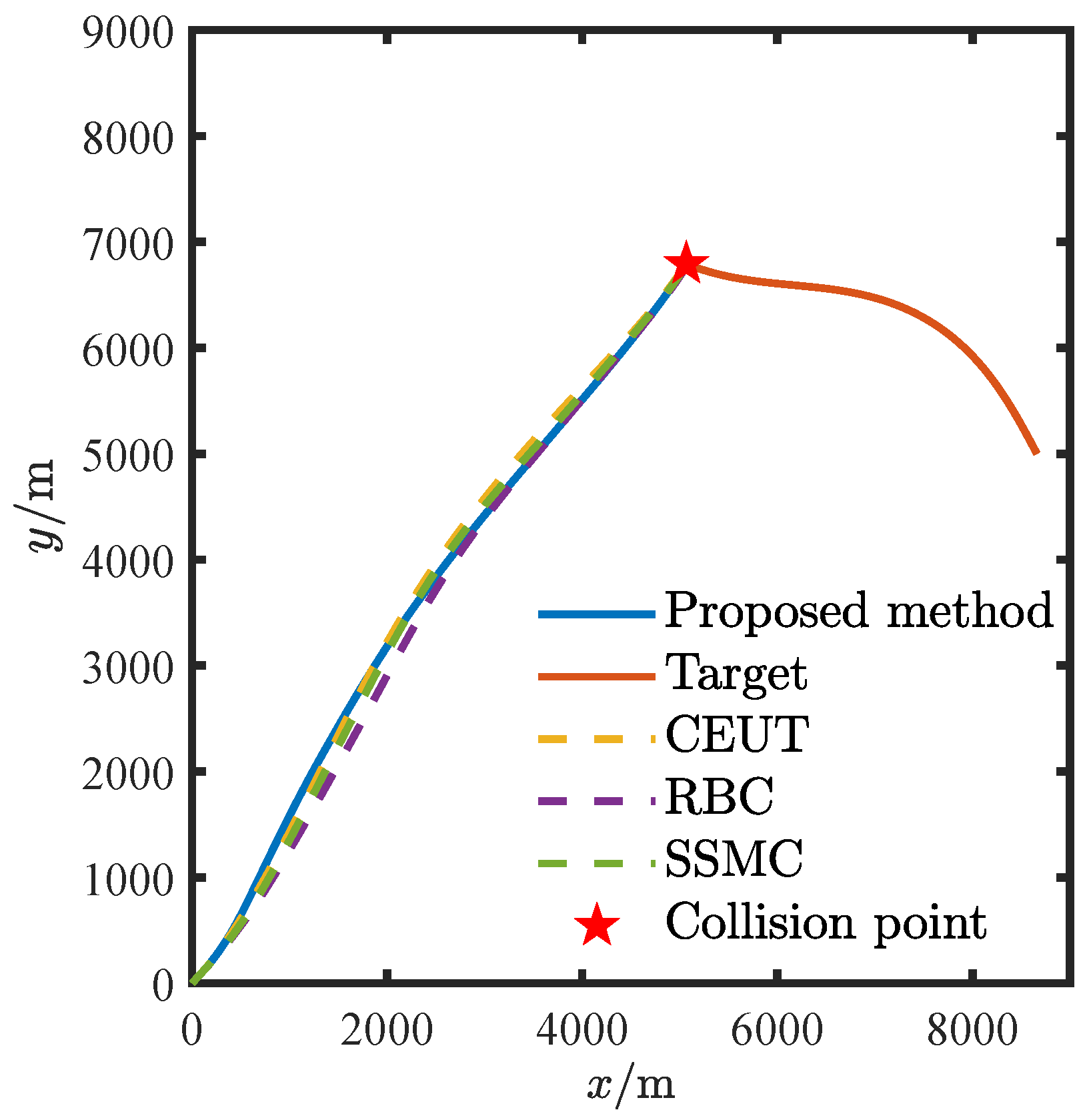
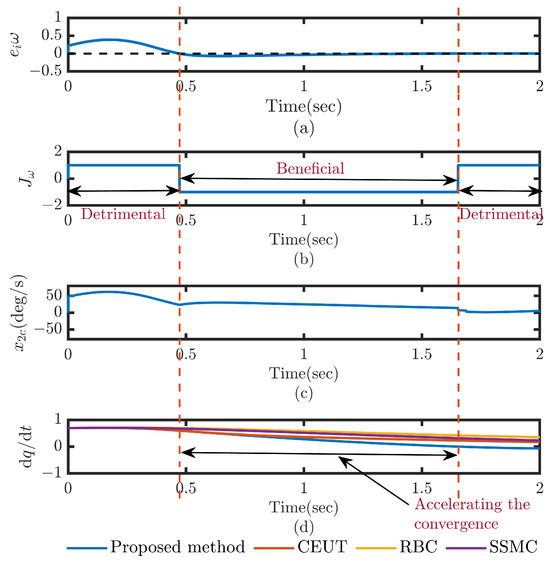
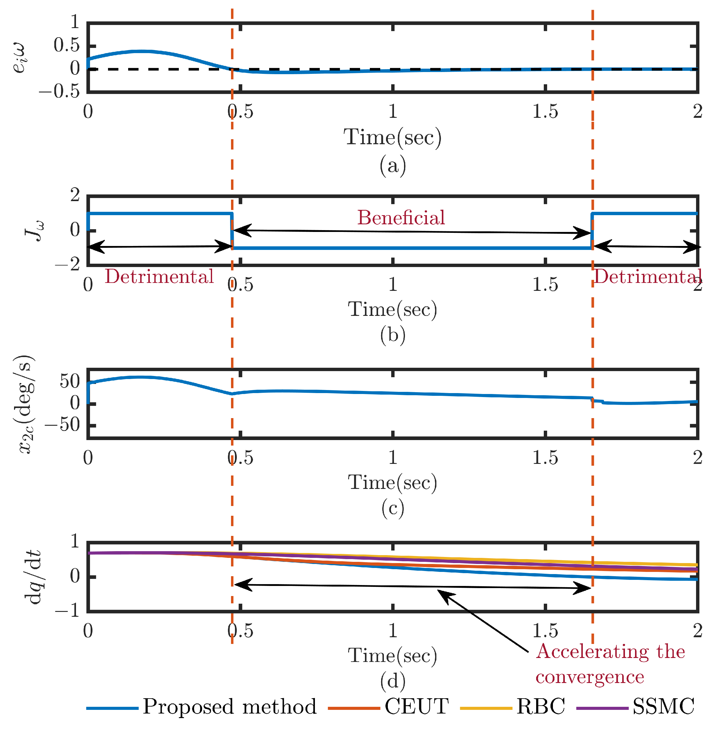
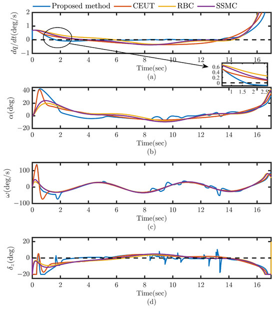
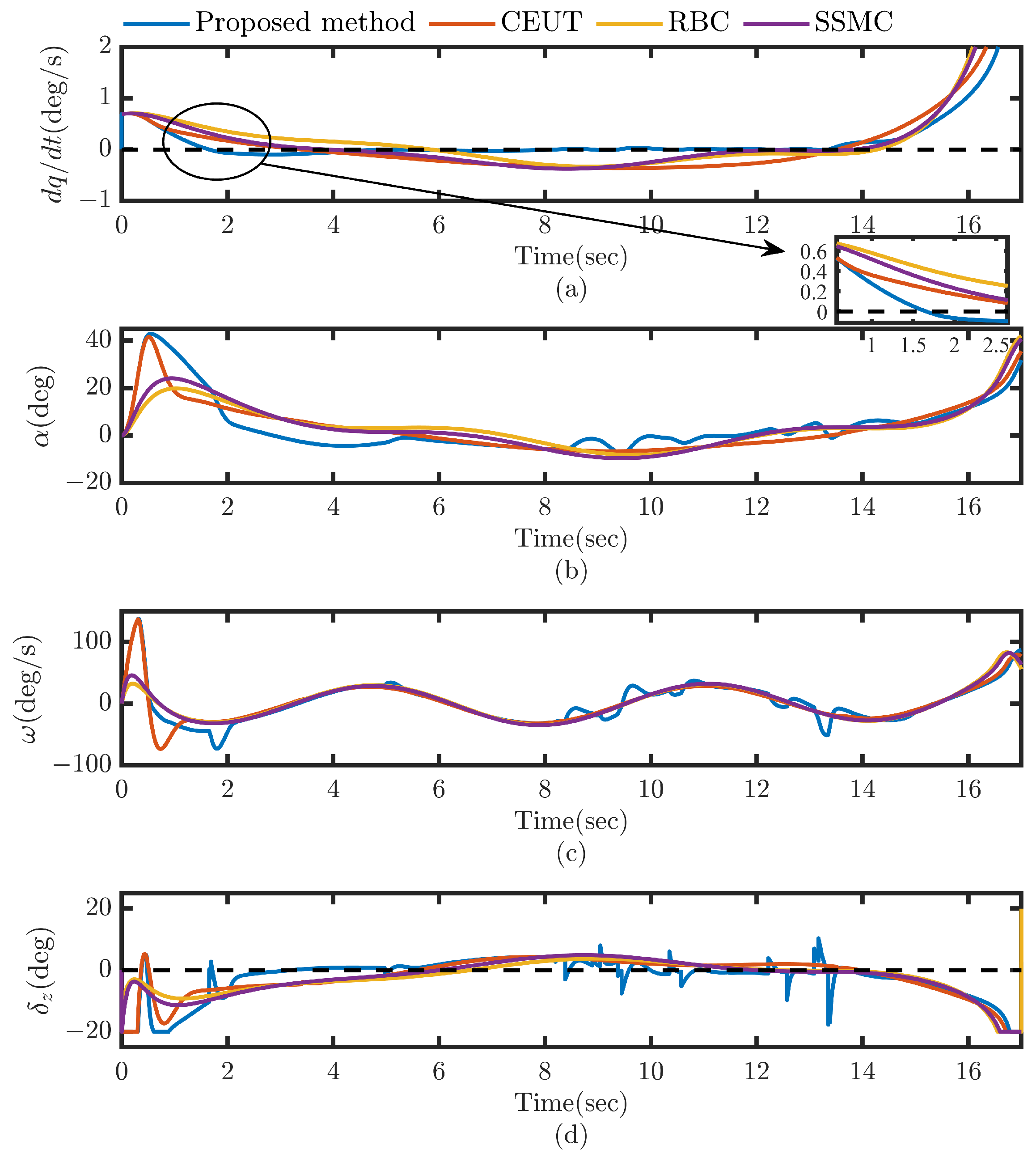
Simulation results under Case 1 are shown in Figure 5, Figure 6 and Figure 7 and Table 2. Figure 5 demonstrates the interception effectiveness of the proposed method and three comparative control methods for flight vehicle–target engagement. The miss distances of all four methods are given in Table 2, and the proposed method achieves the smallest miss distance, confirming its superior interception performance. Figure 6 shows the accelerated convergence mechanism of the proposed method. It is achieved through the convergence rate indicator, which can transform and leverage the influence of model nonlinearities and coupling terms. Based on the indicator, the influence is actively injected into the control laws, causing the faster convergence speed of the LOS angular rate. Figure 7a–d correspond to the LOS angular rate, angle of attack, the pitch angular rate and the rudder deflection, respectively. Comparative analysis in Figure 7a reveals that the proposed method performs markedly faster convergence of LOS angular rate.

Figure 5. The trajectory of flight vehicle and target under Case 1.

Figure 6. Magnification in $t\in [0,2]$ of the flight vehicle’s response curves to demonstrate the convergence rate estimation mechanism. (a) Curve of internal factors imposed on convergence; (b) Measuring and modifying the influence with the convergence rate indicator; (c) Injecting the modified influence into the controller via the convergence rate indicator; (d) Accelerating the convergence and improving the performance of the flight vehicle.

Figure 7. The response curves of the state errors and control input under different methods in Case 1. (a) Curves of LOS angular rate under Case 1; (b) Curves of angle of attack under Case 1; (c) Curves of pitch angular rate under Case 1; (d) Curves of rudder deflection under Case 1.

Table 2. Miss distance comparison under Case 1.

Method	Miss Distance
Proposed Method	0.1220 m
CEUT [6]	0.3778 m
RBC [10]	1.1516 m
SSMC [19]	1.0431 m

To further show the effectiveness of the proposed method, quantitative comparisons of convergence time when the LOS angular rate first enters and remains within an error band of $\pm 0.15\mathrm{deg}/\mathrm{s}$ are performed under two conditions. As shown in Table 3, under nominal condition without disturbances or parameter variations, the proposed method enters the error band at $1.357$ s, outperforming CEUT ($2.162$ s), SSMC ($2.630$ s), and RBC ($3.991$ s). Under condition with additive disturbances ($d_2=0.5sin\left(t\right)\mathrm{rad}$, $d_3=0.5sin\left(t\right)\mathrm{rad}/\mathrm{s}$), target maneuver ($a_T=30sin\left(0.25t\right){\mathrm{m}/\mathrm{s}}^2$) and a 20% increment in aerodynamic coefficients, the proposed method enters the error band at $1.108$ s, whereas CEUT, SSMC, and RBC require $1.690$ s, $2.029$ s, and $3.035$ s, respectively, and only the proposed method sustains stability within the $\pm 0.15\mathrm{deg}/\mathrm{s}$ range after entry. These results quantitatively validate the accelerated convergence and enhanced robustness of the proposed method.

Table 3. Convergence time comparison of different control methods under nominal condition and Case 1 (error band: $\pm 0.15\mathrm{deg}/\mathrm{s}$).

Condition	Control Method	Convergence Time (s)
Nominal Condition	Proposed Method	1.357
	CEUT [6]	2.162
	RBC [10]	3.991
	SSMC [19]	2.630
Case 1	Proposed Method	1.108
	CEUT [6]	1.690
	RBC [10]	3.035
	SSMC [19]	2.029

To further verify the reliability and robustness of the proposed method, Monte Carlo tests are executed in the following cases.

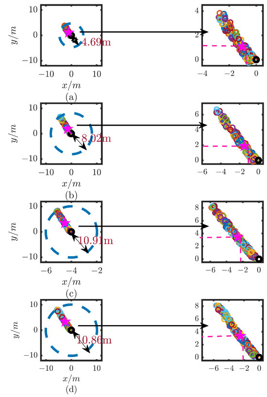
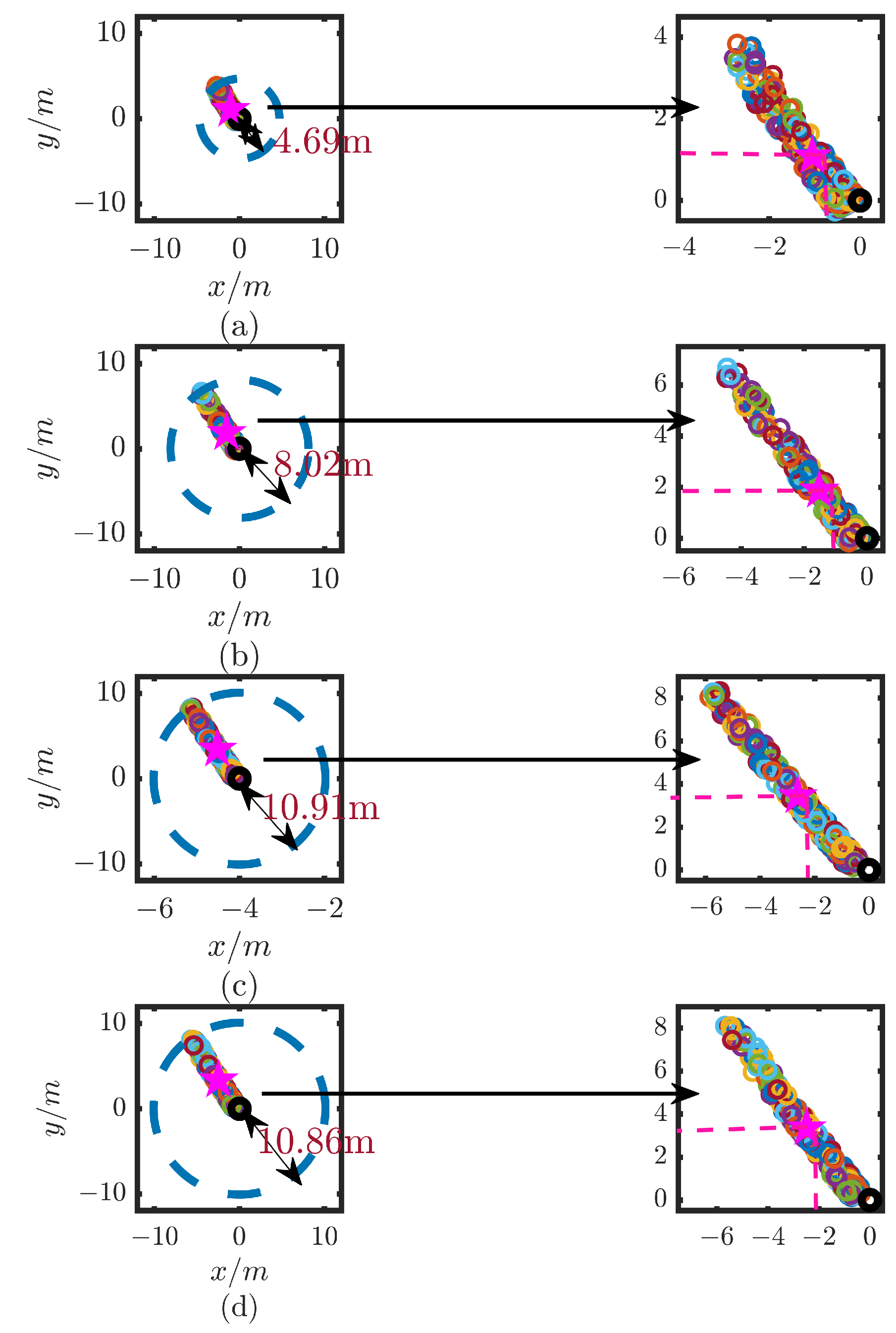
Case 2: Monte Carlo tests are conducted in 300 iterations with all aerodynamic parameters subjected to independent random perturbations within $[-30\%,30\%]$, and additive disturbances and target maneuver are the same value as Case 1.

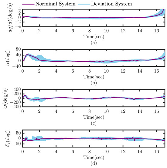
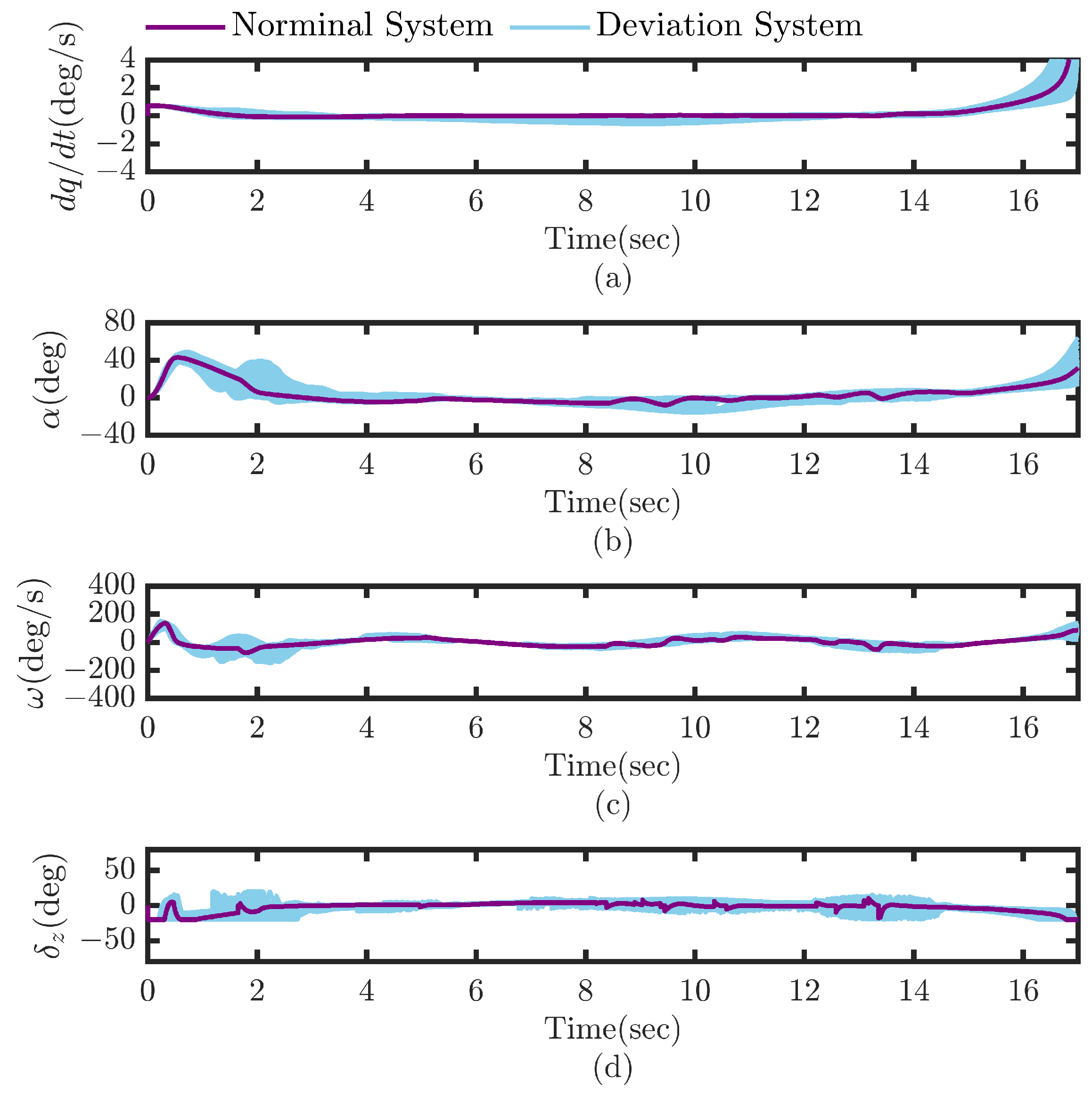
The results of the Monte Carlo tests under Case 2 are presented in Figure 8 and Figure 9 and Table 4. Figure 9 shows that the miss distances of the proposed method are confined within a circle of radius $R=4.69\mathrm{m}$ while those of CEUT, RBC, and SSMC are distributed within $8.02\mathrm{m}$, $10.91\mathrm{m}$, and $10.86\mathrm{m}$, respectively. Table 4 shows that the proposed method has a smaller average miss distance ($1.32\mathrm{m}$) than that of the other three comparative methods, which means that the better interception performance is achieved by the proposed method based on the convergence rate estimation mechanism. Moreover, the state errors and control input of the Monte Carlo simulation are given in Figure 8, and their curves are all near the norminal ones, verifying the effectiveness of the proposed method in suppressing aerodynamic parameter perturbations.

Figure 8. The response curves of the state errors and control input under Case 2. (a) Curves of LOS angular rate under Case 2; (b) Curves of angle of attack under Case 2; (c) Curves of pitch angular rate under Case 2; (d) Curves of rudder deflection under Case 2.

Figure 9. The miss distances of Monte Carlo simulations under Case 2. (a) Proposed method, (b) CEUT, (c) RBC, (d) SSMC.

Table 4. Miss distance comparison under Case 2.

Method	Average Miss Distance
Proposed Method	1.32 m
CEUT [6]	2.05 m
RBC [10]	4.02 m
SSMC [19]	3.76 m

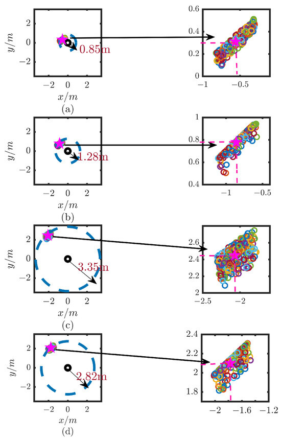
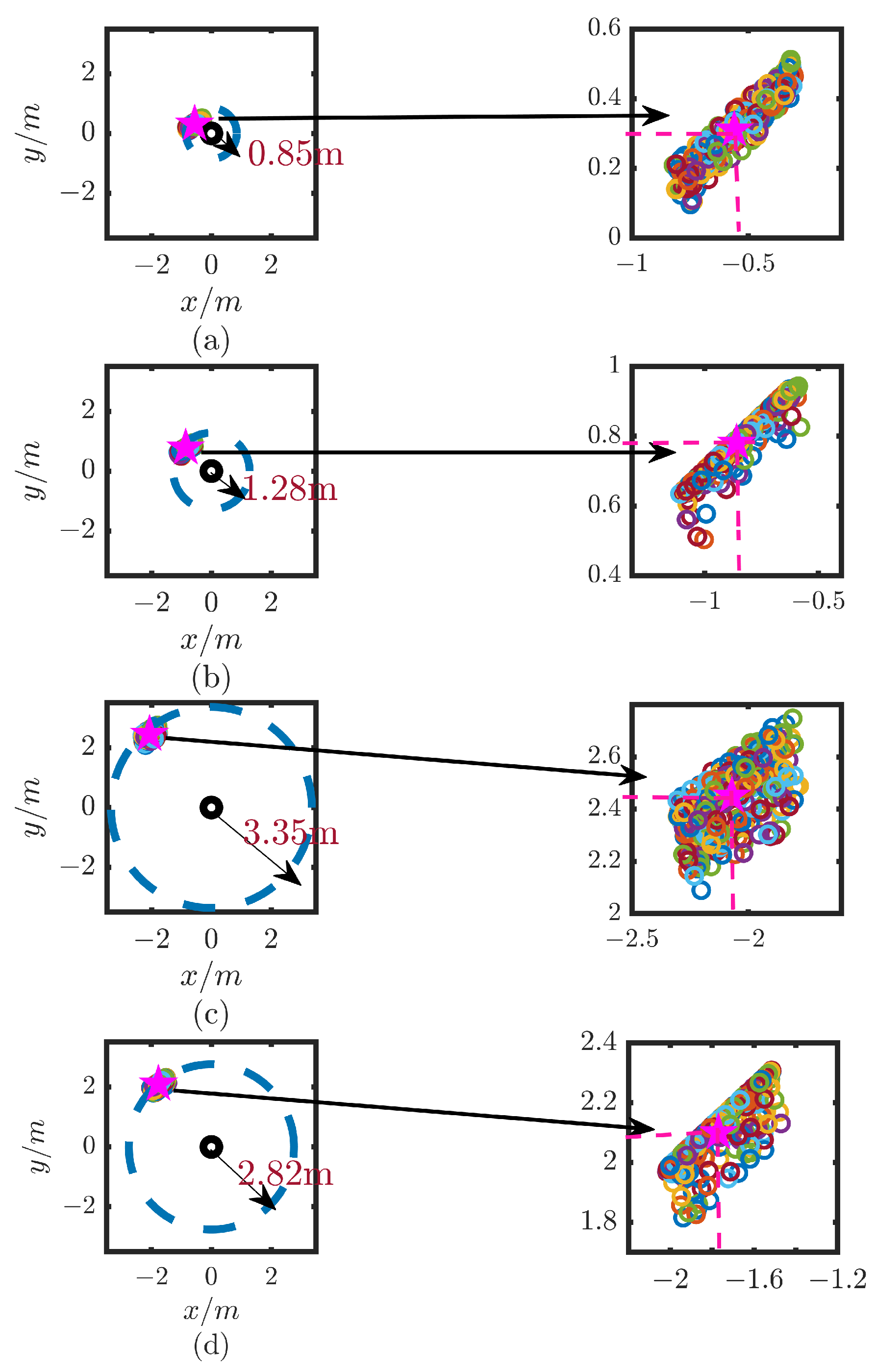
Case 3: The Monte Carlo simulations are performed using the same parameter settings in Case 1, with an additive random deflection $[-45\%,45\%]$ applied to the initial flight path angle ${\theta }_{M0}={45}^{°}$, resulting in ${\theta }_{M0}\in [{25}^{°},{65}^{°}]$.

Figure 10 and Table 5 demonstrate that the proposed fast robust IGC control method outperforms the other three robust control methods, achieving a minimum miss distance of 0.85 m and a minimum average of only 0.66 m. From the analysis of the above simulations under different cases, it can be concluded that the proposed method has the fastest convergence and the best interception performance among the four robust control methods.

Figure 10. The miss distances of Monte Carlo simulations under Case 3. (a) Proposed Method, (b) CEUT, (c) RBC, (d) SSMC.

Table 5. Miss distance comparison under Case 3.

Method	Average Miss Distance
Proposed Method	0.66 m
CEUT [6]	1.17 m
RBC [10]	3.21 m
SSMC [19]	2.75 m

Remark 6.

The simulations in this study employ a fixed step size of 1 $ms$, and the actual average computation time required to solve the controller update at each step is $0.539ms$ on the simulation platform. This leaves a sufficient margin within the 1 ms cycle, ensuring that the real-time requirement is satisfied in the simulations. Therefore, the processing delay does not affect the presented results. The chattering observed in the system response arises from the active exploitation of system nonlinearities and coupling effects to achieve accelerated convergence, representing a conscious trade-off between convergence speed and signal smoothness. In the meanwhile, the chattering frequency is inherently constrained by the practical actuator rate limit of below ${200}^{°}/s$ [20], and both the convergence rate indicator designed with continuous cosine function and first-order filters for smoothing virtual control laws served to alleviate the chattering phenomenon to an engineering acceptable degree.

6. Conclusions

In this paper, a fast robust IGC scheme for flight vehicles based on convergence rate estimation mechanism is proposed, which improves the control performance and interception accuracy of interceptors. The influence of internal factors including model nonlinearities and couplings existing in flight vehicles on convergence are analyzed by the Lyapunov stability theory. Based on the analysis, a convergence rate indicator for flight vehicles is developed to measure the influence of the factors on the convergence, and a convergence rate estimation mechanism is designed to transform the influence, which is actively injected into controllers to accelerate the convergence of interceptors and improve the dynamic performance of the flight vehicles in the interception process. Also, the stability analysis of the closed-loop system is performed via the Lyapunov stability theory. Extensive numerical simulations are conducted to verify the effectiveness of the proposed method, and the results confirm that the fast robust control method for the flight vehicles outperforms three other recently developed robust control methods. Our future work will explore how to design learning-based control methods via the convergence rate estimation mechanism to further optimize and improve the guidance and control performance of flight vehicles.

References

- Lee, Y.; Kim, Y.; Moon, G.; Jun, B.E. Sliding-mode-based missile-integrated attitude control schemes considering velocity change. J. Guid. Control. Dyn. 2016, 39, 423–436. [Google Scholar] [CrossRef] [Scilit]
- Sun, J.; Liu, C. Backstepping-based adaptive dynamic programming for missile-target guidance systems with state and input constraints. J. Frankl. Inst. 2018, 355, 8412–8440. [Google Scholar] [CrossRef] [Scilit]
- Yan, H.; Ji, H. Integrated guidance and control for dual-control missiles based on small-gain theorem. Automatica 2012, 48, 2686–2692. [Google Scholar] [CrossRef] [Scilit]
- Shao, X.L.; Wang, H.L. Back-stepping active disturbance rejection control design for integrated missile guidance and control system via reduced-order ESO. ISA Trans. 2015, 57, 10–22. [Google Scholar] [CrossRef] [Scilit]
- Dong, F.; Zhang, X.; Tan, P. Integrated Guidance and Control Based on Improved Backstepping Method Under Input Saturation and Attitude Angle Constraints. Int. J. Adapt. Control Signal Process. 2025, 39, 74–87. [Google Scholar] [CrossRef] [Scilit]
- Guo, Z.; Yao, L.; Cao, S.; Ding, Y.; Yuan, R.; Huang, L.; Guo, J. Integrated Missile Guidance and Control Scheme Via Coupling Effect Utilization and Transformation Mechanism. IEEE Trans. Aerosp. Electron. Syst. 2025, 61, 2068–2077. [Google Scholar] [CrossRef] [Scilit]
- Li, Z.; Dong, Q.; Zhang, X.; Gao, Y. Impact angle-constrained integrated guidance and control for supersonic skid-to-turn missiles using backstepping with global fast terminal sliding mode control. Aerosp. Sci. Technol. 2022, 122, 107386. [Google Scholar] [CrossRef] [Scilit]
- Ran, M.; Wang, Q.; Hou, D.; Dong, C. Backstepping design of missile guidance and control based on adaptive fuzzy sliding mode control. Chin. J. Aeronaut. 2014, 27, 634–642. [Google Scholar] [CrossRef] [Scilit]
- Huang, H.; Zhao, X.; Zhang, X. Intelligent guidance and control methods for missile swarm. Comput. Intell. Neurosci. 2022, 2022, 8235148. [Google Scholar] [CrossRef] [Scilit]
- Wang, X.; Lan, G.; Lu, H.; Huang, X. Three-dimensional integrated guidance and control with input saturation and impact angle constraints. Aerosp. Sci. Technol. 2022, 127, 107727. [Google Scholar] [CrossRef] [Scilit]
- Li, Z.; Zhang, X.; Zhang, H.; Zhang, F. Three-dimensional approximate cooperative integrated guidance and control with fixed-impact time and azimuth constraints. Aerosp. Sci. Technol. 2023, 142, 108617. [Google Scholar] [CrossRef] [Scilit]
- Wang, X.; Chen, Z.; Yang, G. Finite-time-convergent differentiator based on singular perturbation technique. IEEE Trans. Autom. Control 2007, 52, 1731–1737. [Google Scholar] [CrossRef] [Scilit]
- Zhao, L.; Yu, J.; Lin, C.; Ma, Y. Adaptive neural consensus tracking for nonlinear multiagent systems using finite-time command filtered backstepping. IEEE Trans. Syst. Man Cybern. Syst. 2018, 48, 2003–2012. [Google Scholar] [CrossRef] [Scilit]
- Vafamand, N. Adaptive robust neural-network-based backstepping control of tethered satellites with additive stochastic noise. IEEE Trans. Aerosp. Electron. Syst. 2020, 56, 3922–3930. [Google Scholar] [CrossRef] [Scilit]
- Wang, P.; Zhang, X.; Zhu, J. Integrated missile guidance and control: A novel explicit reference governor using a disturbance observer. IEEE Trans. Ind. Electron. 2019, 66, 5487–5496. [Google Scholar] [CrossRef] [Scilit]
- Zhang, K.; Zhang, Z.; Han, Z. Optimal guidance law design for three-dimensional trajectory tracking of missiles based on fixed-gain disturbance observer. ISA Trans. 2023, 143, 298–312. [Google Scholar] [CrossRef] [Scilit] [PubMed]
- Ji, Y.; Lin, D.; Pei, P.; Shi, X.; Wang, W. Robust partial integrated guidance and control approaches for maneuvering targets. Int. J. Robust Nonlinear Control 2019, 29, 6522–6541. [Google Scholar] [CrossRef] [Scilit]
- Guo, J.; Li, Y.; Zhou, J. Qualitative indicator-based guidance scheme for bank-to-turn missiles against couplings and maneuvering targets. Aerosp. Sci. Technol. 2020, 106, 106196. [Google Scholar] [CrossRef] [Scilit]
- Guo, Z.; Ma, Q.; Guo, J.; Zhao, B.; Zhou, J. Performance-involved coupling effect-triggered scheme for robust attitude control of HRV. IEEE/ASME Trans. Mech. 2020, 25, 1288–1298. [Google Scholar] [CrossRef] [Scilit]
- Guo, Z.; Guo, J.; Chang, J.; Zhou, J. Coupling effect-triggered control strategy for hypersonic flight vehicles with finite-time convergence. Nonlinear Dyn. 2019, 95, 1009–1025. [Google Scholar] [CrossRef] [Scilit]
- Markham, K.C. Solutions of Linearized Proportional Navigation Equation for Missile with First-Order Lagged Dynamics. J. Guid. Control. Dyn. 2024, 47, 589–596. [Google Scholar] [CrossRef] [Scilit]
- Wen, Q.; Wang, M.; Li, X.; Chang, Y. Learning-based design optimization of second-order tracking differentiator with application to missile guidance law. Aerosp. Sci. Technol. 2023, 137, 108302. [Google Scholar] [CrossRef] [Scilit]
- Zhang, T.P.; Ge, S.S. Adaptive dynamic surface control of nonlinear systems with unknown dead zone in pure feedback form. Automatica 2008, 44, 1895–1903. [Google Scholar] [CrossRef] [Scilit]
- Liu, H.; Pan, Y.; Cao, J. Composite learning adaptive dynamic surface control of fractional-order nonlinear systems. IEEE Trans. Cybern. 2019, 50, 2557–2567. [Google Scholar] [CrossRef] [Scilit] [PubMed]
- Ma, Q.; Xu, X.; Zhang, R.; Xiong, Q.; Zhang, X.; Zhang, X. Robust consensus control of nonlinear multi-agent systems based on convergence rate estimation. Int. J. Robust Nonlinear Control 2023, 33, 2003–2021. [Google Scholar] [CrossRef] [Scilit]
- Yu, S.; Yu, X.; Shirinzadeh, B.; Man, Z. Continuous finite-time control for robotic manipulators with terminal sliding mode. Automatica 2005, 41, 1957–1964. [Google Scholar] [CrossRef] [Scilit]
- Bu, X.W.; Wu, X.Y.; Chen, Y.X.; Bai, R.Y. Design of a class of new nonlinear disturbance observers based on tracking differentiators for uncertain dynamic systems. Int. J. Control. Autom. Syst. 2015, 13, 595–602. [Google Scholar] [CrossRef] [Scilit]
- Kim, K.S.; Rew, K.H.; Kim, S. Disturbance observer for estimating higher order disturbances in time series expansion. IEEE Trans. Autom. Control 2010, 55, 1905–1911. [Google Scholar]
Disclaimer/Publisher’s Note: The statements, opinions and data contained in all publications are solely those of the individual author(s) and contributor(s) and not of MDPI and/or the editor(s). MDPI and/or the editor(s) disclaim responsibility for any injury to people or property resulting from any ideas, methods, instructions or products referred to in the content. |
© 2026 by the authors. Licensee MDPI, Basel, Switzerland. This article is an open access article distributed under the terms and conditions of the Creative Commons Attribution (CC BY) license.