Deep-Reinforcement-Learning-Enhanced Kriging Modeling Method with Limit State Dominant Sampling for Aeroengine Structural Reliability Analysis

Abstract

Reliability analysis of aeroengine structures is a critical task in aerospace engineering, but traditional methods often face challenges of low computational efficiency and insufficient accuracy when dealing with complex, high-dimensional, and nonlinear problems. This paper proposes a novel reliability assessment method (AC-Kriging) based on the Actor–Critic network and Kriging surrogate models to address these issues. The Actor network optimizes the sampling strategy for design variables, making sampling more efficient. The Critic network assesses the reliability of these samples to ensure accurate results, while a Kriging surrogate model replaces expensive finite element simulations and cuts computational cost. Three case studies demonstrate that AC-Kriging significantly outperforms traditional methods in both sampling efficiency and reliability estimation accuracy. This research provides an efficient and reliable solution for reliability analysis of aeroengine structures, with important theoretical and engineering application value. Three case studies demonstrate that AC-Kriging significantly outperforms traditional methods in both sampling efficiency and reliability-estimation accuracy, requiring only 52–147 samples to achieve comparable accuracy while maintaining the relative failure probability error within 0.87–7.27%. This research provides an efficient and reliable solution for the reliability analysis of aeroengine structures.

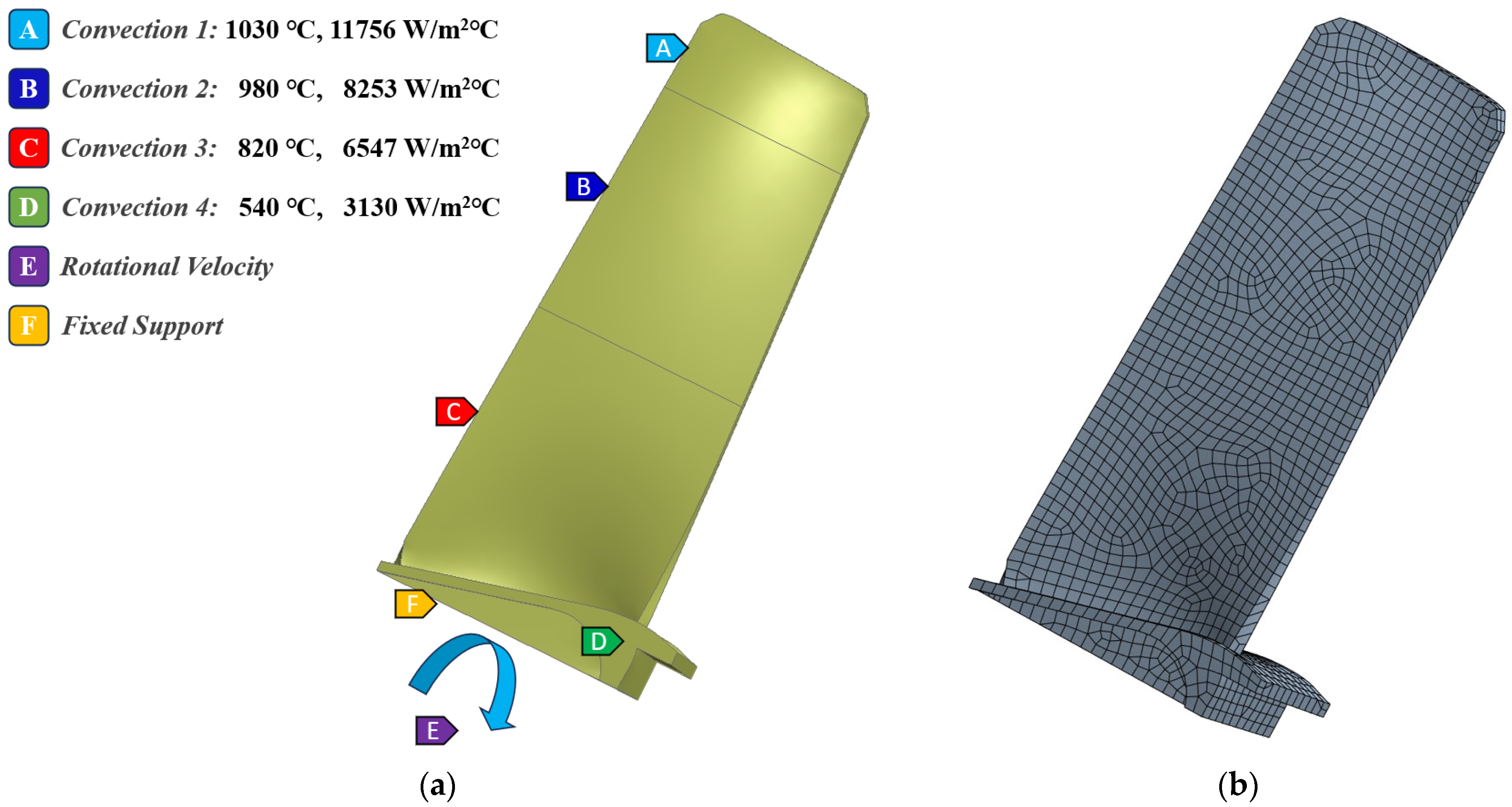
1. Introduction

Structural reliability analysis of aeroengine components represents one of the most critical challenges in aerospace engineering, directly impacting flight safety, operational efficiency, and economic viability of modern aviation systems [1]. It is significant to quantify the structural failure probability under complex working conditions for ensuring structural reliability and safety. In the past few decades, there have been many works about structural failure probability estimation [1,2,3]. As the critical power components of aircraft, aeroengine structures like turbine blisks are typically exposed to the uncertain environment of high temperature, severe pressure differentials and alternating loads, which represent challenges to the accurate assessment of fatigue failure probability [4,5]. To quantify the structural failure probability, the equation can be defined as follows [6]:

$$P_f={\displaystyle {\int }_{g(\mathit{x})\le 0}f(\mathit{x})d\mathit{x}}$$

(1)

where x = [x₁, x₂, x₃, …, x_n] represents the input vector of random variables including material properties, loads settings and fatigue parameters; g(·) is the structural limit state function (LSF) or failure surface, which is shown as structural failure when g(x) ≤ 0; f(·) denotes the joint probability density function associated with the random variables x. However, it is an intractable analytically to calculate the failure probability of structures under complex operating conditions by the integral Equation (1). Therefore, numerical surrogate methods are needed to balance the computational efficiency with estimation accuracy.

Traditional reliability analysis methods, including the first-order reliability method (FORM), second-order reliability method (SORM), etc., approximate the LSF by Taylor series expansion around the design of points (DoPs) [7,8]. Despite the computational efficiency advantages, FORM and SORM are limited to precision accuracy in high-dimensional nonlinear problems by low-order polynomial approximations. Moreover, the fatigue failure mechanisms of turbine blisks result in non-convex failure domains, which violate the assumptions of FORM/SORM [9]. Monte Carlo Simulation (MCS), as one of the most significant numerical simulation methods, provides a gold standard for failure probability estimation by directly sampling the probability space [10]. Based on the MCS, the estimation of failure probability is described as follows:

$${\widehat{P}}_f\approx {\displaystyle \frac{1}{N}}{\displaystyle \sum _{i=1}^{N}I[g(\mathit{x})\le 0]}={\displaystyle \frac{N_f}{N}} s.t. I[g(\mathit{x})]=\left\{\begin{array}{c}0,g\left(\mathit{x}\right)\le 0\\ 1,g\left(\mathit{x}\right)>0\end{array}\right.$$

(2)

where I[·] is the indicator function of g(x), which equals 1 in case of structural failure; otherwise, it is 0; N is the total number of simulation samples; and N_f is the theoretical minimum simulation number with a relative error ε of P_f, and it is as follows:

$$N\ge {\displaystyle \frac{z_{\alpha /2}^2(1-{\widehat{P}}_f)}{{\epsilon }^2\cdot {\widehat{P}}_f}}$$

(3)

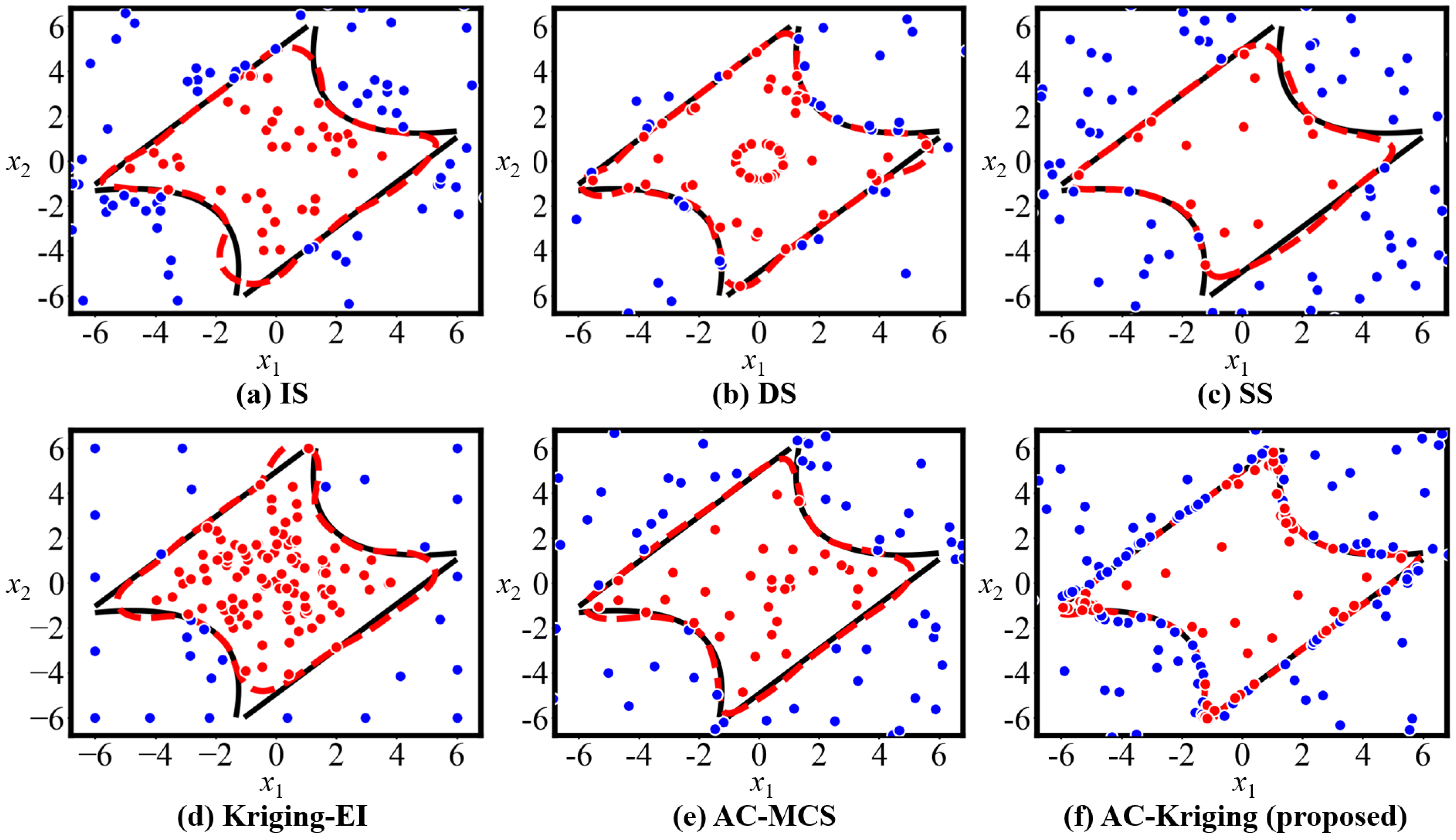
where z is the normal distribution; α/2 is the quantile of z, and 1 − α is used to define the confidence interval. However, prohibitively high computational demands in the theoretical random sampling process of MCS are needed, which exponentially increase with the precision of failure probability. The typical structural failure probability of aeroengines is usually less than 1 × 10⁻⁵, which is needed for millions of high-fidelity finite element (FE) simulations in MCS, far beyond the acceptable range in practical projects. To address this issue, advanced reliability analysis methods, such as importance sampling (IS), directional sampling (DS) and subset simulation (SS), have been developed to estimate small probability of failure [11,12,13]. However, IS faces challenges in accurately selecting the importance function and solving high-dimensional complex failure regions, and SS suffers from high computational cost in each subset and sensitivity to initial samples.

To address the above-mentioned problems, machine learning (ML)-based surrogate modeling has been applied to fit complex implicit LSF and calculate failure probability in structural reliability analysis problems, which has become one of the current research hotspots [14,15,16,17]. Recent studies demonstrate extensive applications of surrogate models in structural reliability analysis, such as polynomial chaos expansions [18], support vector machines [19], artificial neural networks (ANNs) [20], and Kriging models [21,22]. Sun et al. developed a method using LIF, MCMC and MC to update the Kriging model and improve efficiency in structural reliability analysis [21]. Qian et al. proposed a time-variant reliability method for an industrial robot rotate vector reducer with multiple failure modes using a Kriging model [22]. Vazirizade et al. introduced an ANN-based method to reduce the computational effort required for reliability analysis and damage detection [23]. Yang et al. enhanced sparse polynomial chaos expansion accuracy through sequential sample point extraction, successfully applying it to slope reliability analysis [24]. Gaussian processes have been particularly well investigated for structural reliability analysis due to their statistical learning capabilities [25,26,27]. However, it is critical to select the DoPs by a sampling method for training the surrogate models. The lack of training samples near the LSF will limit the accuracy and efficiency of surrogate models. For complex structures like aeroengines, it is difficult to construct an accurate model of the LSF by one-time sampling to obtain design points. Therefore, how to optimize sampling and improve the accuracy of models near the LSF has become one key research issue in structural reliability analysis.

Recently, active sampling methods have become interesting in the field of structural reliability analysis due to the advantages in enhancing accuracy of surrogate models and computational efficiency [20,28,29]. The active selection of samples greatly reduces the computational cost by maximizing contributions of failure probability evaluation. For example, Ling et al. [6] proposed a method combining adaptive Kriging with MCS to efficiently estimate the failure probability function; Wang et al. developed a new active learning method for estimating the failure probability based on a penalty learning function [30]; and Yuan et al. proposed an efficient reliability method for structural systems with multiple failure modes, developing a new learning function based on the system structure function to select added points from a system perspective [20]. These methods only require calling the real model once in each iteration, significantly improving computational efficiency. However, it is easy to fall into local optima in active-learning-based modeling due to variance estimation bias near nonlinear failure domain boundaries causing redundant samples or missing key areas. To address the above-mentioned problem, failure probability sensitivity-based sampling methods are proposed [31,32]. Dang et al. proposed a Bayesian active learning line sampling to improve the epistemic uncertainty about failure probability [33]. Moustapha et al. developed an active learning strategy designed for solving the presence of multiple failure modes and the uneven contribution to failure [34]. Liu et al. integrated the classical active Kriging-MCS and adaptive linked importance sampling to establish a novel reliability analysis in the extremely small failure probability [35]. However, current active sampling approaches face two significant challenges that limit their effectiveness: (1) the majority of existing techniques rely on fixed learning functions that cannot dynamically adjust their sampling strategies based on evolving problem understanding or provide adaptive feedback for sample quality assessment; (2) the computational burden grows substantially with increasing problem dimensionality, creating practical barriers for implementation in high-dimensional engineering applications typical of complex structural systems.

Deep reinforcement learning (DRL), through the unique “state-action-reward” interactive framework, achieves autonomous optimization and iterative evolution of strategies, providing a new paradigm for active learning in structural reliability analysis. Recently, DRL has made significant breakthroughs in various fields, including the successes of AlphaGo [36], Deep Q-Networks (DQNs) [37] and large language models (like ChatGPT-3, Deepseek-R1) [38,39]. Many studies on DRL-based structural reliability analysis have emerged; for instance, Xiang et al. proposed a DRL-based sampling method for structural reliability assessment [40]; Guan et al. developed high-accuracy structural dominant failure modes and self-play strategy searching methods based on DRL [41,42]. Wei et al. introduced a general DRL framework for structural maintenance policy [43]. Li et al. proposed an efficient optimization method of the base isolation systems and shape memory alloy inverter using different DRL algorithms [44]. The DRL-based reliability analysis methods have shown potential, but there are several challenges in the LSF modeling process: (1) It is not easy to converge in the training process of deep learning network. (2) The reward function settings still need improvement to reasonably select DoPs. However, DRL is still in the exploratory stage in structural reliability analysis, and its potential has been shown.

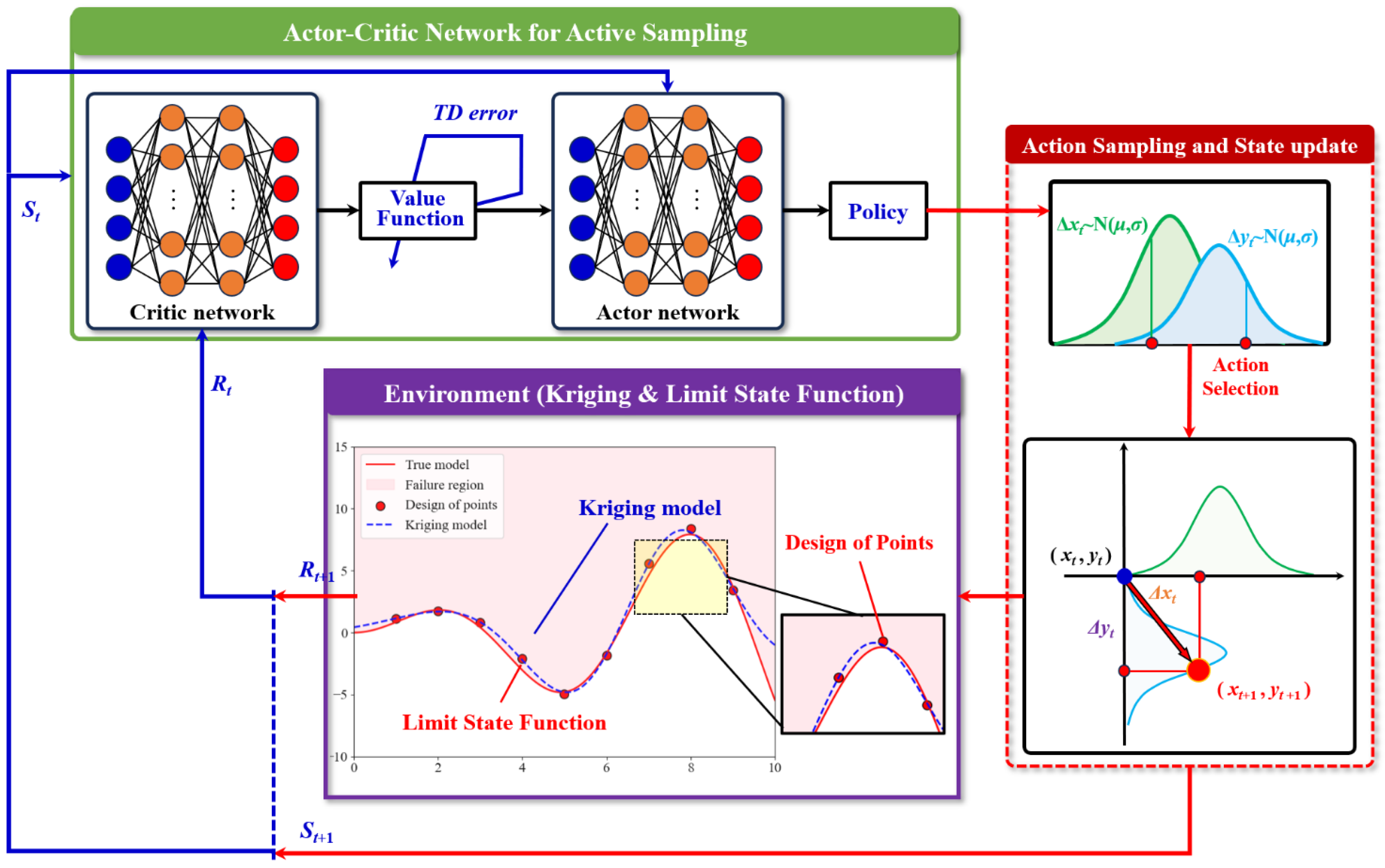
The critical gap in the current literature lies in the absence of a theoretically grounded, computationally efficient, and practically robust method that can adaptively optimize sampling strategies based on evolving the understanding of the limit state function, provide theoretical convergence guarantees for failure probability estimation accuracy, scale effectively to high-dimensional problems typical in aerospace engineering, balance multiple objectives including accuracy, efficiency, and computational budget constraints, and integrate seamlessly with established surrogate modeling frameworks. To solve the above-mentioned issues, an Actor–Critic network-enhanced Kriging method (AC-Kriging) is proposed to obtain the positive DoPs through DRL-based active searching and establish the surrogate LSF for structural reliability evaluation. Specifically, in the application of AC-Kriging, the following steps are carried out: (1) Firstly, an initial Kriging model is constructed using a Latin hypercube sampling (LHS)-generated DoPs to approximate the structural LSF. (2) The Actor network identifies candidate points within the DoPs, while the Critic network evaluates their potential contributions through global-local reward functions based on the Kriging model’s prediction errors, thereby selecting the next optimal sampling point. (3) The accuracy of the Kriging model is iteratively evaluated, and the convergence of reliability analysis is monitored until the dual convergence criteria (model precision and algorithmic stability) are satisfied. The AC-Kriging method aims to develop an efficient and accurate structural reliability analysis framework by the seamless integration of Kriging modeling and Actor–Critic reinforcement learning networks.

The primary contributions of this paper to the field of structural reliability analysis are as follows:

(1)

This study introduces a comprehensive framework that combines Actor–Critic reinforcement learning with Kriging surrogate modeling for structural reliability analysis, enabling dynamic and intelligent sample selection that adapts to the evolving understanding of limit state boundaries throughout the analysis process.

(2)

The proposed continuous state–action representation effectively addresses the curse of dimensionality that affects traditional active sampling methods, achieving improved computational scaling with problem size and making it more suitable for complex aerospace engineering applications.

(3)

This research develops dual convergence criteria that monitor both Kriging model precision and algorithmic stability, providing a systematic approach for determining when sufficient sampling accuracy has been achieved in the reliability analysis process.

(4)

The AC-Kriging method optimizes multiple competing objectives by its reward function design, addressing the real-world constraints faced by aerospace engineers while providing a theoretical foundation for integrating deep reinforcement learning principles with established surrogate modeling frameworks.

The remainder of this paper is structured as follows: Section 2 introduces the theoretical basis of active sampling based on AC networks, Section 3 elaborates on the proposed AC-Kriging method, Section 4 verifies the accuracy and efficiency of the method through theoretical and engineering aeroengine structural reliability analysis, and Section 5 provides the conclusions.

2. Deep Reinforcement Learning

DRL is a hybrid algorithm framework integrating deep learning with reinforcement learning principles to enable autonomous decision-making in high-dimensional state spaces [45]. It is skilled at solving the sequential decision problem by trial and error of an agent in a complex environment. Based on the learning strategy, the final objective would be achieved by the DRL output continuous action of an agent. To evaluate the actions of agents, the rewards calculated by a specific reward function are specified according to each action. DRL aims to maximize the cumulative rewards by combining the rewards of each action and final reward upon task completion, along with a punishment function for undesired actions. Unlike supervised learning, the DRL model is trained by interactive data with rewards instead of diverse labeled data. In addition, the agent is represented by a deep neural network trained by multiple episodes, and each episode contains numerous steps.

As illustrated in Figure 1, DRL is governed by Markov decision process (MDP) in the training process, which provides a basic mathematical framework for solving the decision-making problems, with uncertainty and long-term cumulative rewards [46]. MDP usually consists of five elements (S, A, R, P, γ), in which S is all the possible states or actual states of agent in the environment; A is the actions of agent; R is the reward obtained by agent after one action a ∈ A in one state s ∈ S; P is the state transition probability function, which determines the next S’ given state S = s and action A = a; and γ is the discount rate, which determines the importance of a future reward.

In reinforcement learning, at time step t, s_t represents the state of one agent, and a_t represents the action adopted by one agent in state s_t. According to the reward function r(s,a), the agent receives the reward r_t and reaches the next state s_t+1. The trajectory of the agent in a game is recorded as follows:

$$S_1,A_1,R_1;S_2,A_2,R_2;\cdots ;S_t,A_t,R_t;\cdots ;S_n,A_n,R_n$$

(4)

where n is the step number of one game; S_t, A_t and R_t are the t-th state, action and reward of agent, respectively. In addition, suppose state transitions have Markov properties, namely:

$$P\left(S_{t+1}|S_t,A_t\right)=P\left(S_{t+1}|S_1,A_1,S_2,A_2,\cdots S_t,A_t\right)$$

(5)

The action taken by one agent is determined by the policy function π(a|s). The probability of an agent taking action a in state s is π(a|s) = P[S = s, A = a]. The agent is trained to maximize the expectation of the cumulative discounted return U_t which is defined as follows:

$$U_t=r_t+\gamma \cdot r_{t+1}+{\gamma }^2\cdot r_{t+2}+{\gamma }^3\cdot r_{t+3}+\cdots +{\gamma }^{T-t}\cdot r_T$$

(6)

where T is the last step of each step, and r_i is the reward obtained by the agent at each time step. U_t is a variable that includes future actions and states, with inherent randomness.

Taking the expectation of U_t yields the action-value function Q_π:

$$Q_{\pi }\left(s_t,a_t\right)={\mathbb{E}}_{S_{t+1},A_{t+1},\cdots ,S_n,A_n}\left[U_t|S_t=s_t,A_t=a_t\right]$$

(7)

where S_t = s_t and A_t = a_t are the observed values of S_t and A_t, respectively. Q_π depends on t-th state s_t and action a_t, not on state s_t+1 and action a_t+1 from t + 1 step, because the random variables are eliminated by expectation. To eliminate the influence of strategy policy π, the optimal action-value function Q* is described as follows:

$$Q^{*}\left(s_t,a_t\right)=\underset{\pi }{\max }{Q}_{\pi }\left(s_t,a_t\right), \forall s_t\in S, a_t\in A.$$

(8)

where the best policy function is selected as follows:

$${\pi }^{*}=\underset{\pi }{\mathrm{argmax}}{Q}_{\pi }\left(s_t,a_t\right) \forall s_t\in S, a_t\in A.$$

(9)

which illustrates Q* depends on s_t and a_t.

To quantify the chances of winning the game, the state-value function is defined as follows:

$$V_{\pi }\left(s_t\right)={\mathbb{E}}_{A_t~\pi \left(\cdot |s_t\right)}\left[Q_{\pi }\left(s_t,A_t\right)\right]={\displaystyle \sum _{a\in A}\pi \left(a|s_t\right)\cdot Q_{\pi }\left(s_t,a\right)}$$

(10)

where A_t is eliminated as a random parameter.

$$V_{\pi }\left(s_t\right)={\mathbb{E}}_{A_t,S_{t+1},A_{t+1},\cdots ,S_n,A_n}\left[U_t|S_t=s_t\right]$$

(11)

where the expectation eliminates the dependence of U_t on the random variables A_t, S_t+1, A_t+1, …, S_n, A_n. The greater the state value, the higher the expected return. State value can be used to evaluate the quality of policy π and state s_t.

Reinforcement learning aims to learn a policy function π(a|s) to maximize cumulative discounted rewards. Because directly computing the action-value function Q_π(s,a) and state-value function V_π(s) is often infeasible, DRL employs a deep neural network (DNN) to approximate these functions. For instance, DQNs use neural networks to estimate Q_π(s,a), policy gradient methods directly optimize the policy function parameters, and Actor–Critic methods combine both by using neural networks to approximate both the policy and value functions.

3. Proposed AC-Kriging Method

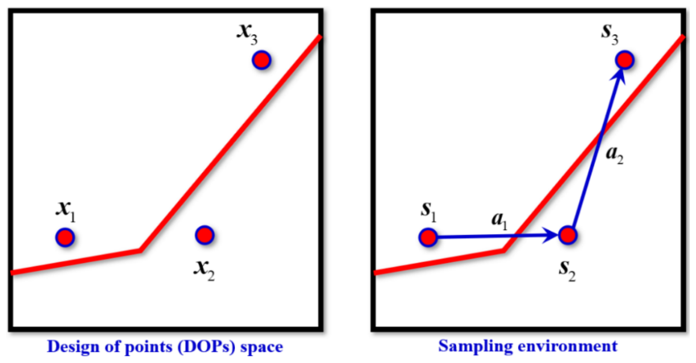
In this study, the AC-Kriging method is proposed for efficient structural reliability analysis, integrating the Actor–Critic reinforcement learning framework with the Kriging model to optimize the selection of experimental sampling points, aiming to accurately approximate the limit state surface while reducing computational cost. As illustrated in Figure 2, the AC-Kriging method establishes correspondences between reliability analysis and the reinforcement learning paradigm: the sampling space represents the environment state, the deep neural network serves as the agent, and the selection of experimental points corresponds to actions.

Step 1: The Kriging model provides essential information about the current approximation of the limit state function.

Step 2: The AC-Kriging method consists of two key networks: (1) an Actor network that determines the optimal location for the next experimental point based on current information, and (2) a Critic network that evaluates the expected contribution of selected points to reliability assessment accuracy. Both networks share initial convolutional layers that extract relevant features from the sampling domain representation, and these features are subsequently processed through fully connected layers to generate either sampling decisions or value estimations.

Step 3: The method operates iteratively, with each cycle involving the extraction of state information from the current Kriging model, selection of a new experimental point, evaluation of the true limit state function at this point, updating of the Kriging surrogate model, and calculation of rewards to refine the neural network parameters.

Through this process, the AC-Kriging method overcomes the limitations of traditional sampling methods by adaptively learning optimal sampling strategies for various structural reliability problems.

3.1. Environment and State Definition

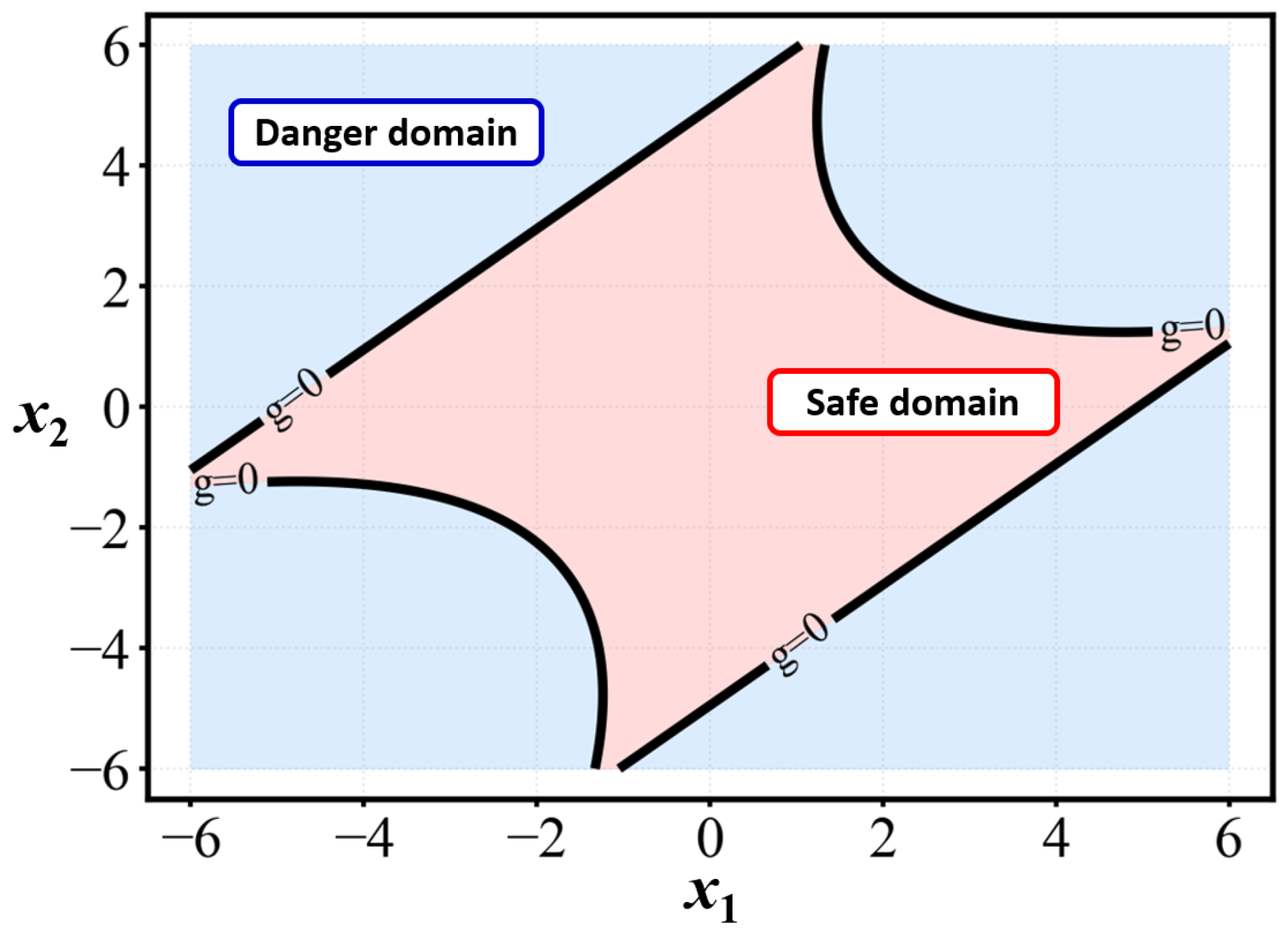
To effectively transform structural reliability analysis into a reinforcement learning problem, the environment is represented as the n-dimensional design space x ∈ Rⁿ, where random variables follow their respective probability distributions. The limit state function (LSF) g(x) partitions this space into failure (g(x) < 0) and safe (g(x) ≥ 0) domains.

3.1.1. State Space Design

In traditional reinforcement learning frameworks, state representations often rely on discretized sampling spaces, which can lead to excessive computational complexity when dealing with high-dimensional problems. To overcome this limitation, the AC-Kriging method proposes a continuous state representation that efficiently captures the essential information needed for reliability analysis. The state space is defined as a two-dimensional continuous space, where each state, s ∈ Rⁿ, represents the spatial coordinates of an agent. Specifically, s = [x₁, x₂, …, x_n], with x_i denoting the agent’s position along the respective axes.

3.1.2. Action Space Design

The action space is a continuous space in Rⁿ, corresponding to the displacement vector an agent can execute. Formally, an action a = [Δx₁, Δx₂, …, Δx_n], where Δx_i ∈ [−1, 1] in Figure 3. This range allows for flexible movement in any direction within the environment while maintaining control over the scale of displacement, ensuring that the agent can perform both fine and coarse adjustments to its position as dictated by the boundary exploration strategy.

3.1.3. Reward Function Design

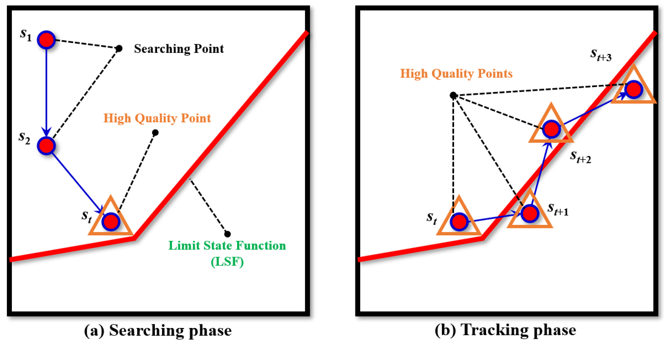
As shown in Figure 4, the AC-Kriging sampling process consists of two phases: in the searching phase (a), the agent starts from random positions to locate the LSF and identify high quality (HQ) points; in the tracking phase (b), the agent initializes from the discovered HQ point to systematically extract more sampling points along the LSF, achieving efficient boundary-following for structural reliability analysis.

In t-step, the reward function is a composite objective function designed to guide the agent’s learning process through a multi-faceted incentive structure, mathematically formulated as follows:

$${\mathit{R}}_k\left(\mathit{s},\mathit{a}\right)=a_1{\mathit{r}}_{\mathrm{edge}}\left(\mathit{s}\right)+a_2{\mathit{r}}_{\mathrm{movement}}\left(\mathit{s},\mathit{a}\right)+a_3{\mathit{r}}_{\mathrm{exploration}}\left(\mathit{s}\right)+a_4{\mathit{r}}_{\mathrm{keep}}\left(\mathit{s}\right)$$

(12)

where the coefficients a₁, a₂, a₃ and a₄ are weighting factors that balance the influence of each reward component, determined through empirical tuning to optimize the agent’s performance in the boundary exploration task.

The reward function comprises four distinct components, each addressing a specific aspect of the boundary-following behavior, which are defined as follows:

(1)

The edge proximity reward is defined as follows:

$${\mathit{r}}_{\mathrm{edge}}\left(\mathit{s}\right)=\exp \left(-\left|\mathit{g}\left(\mathit{s}\right)\right|\right)$$

(13)

which decays exponentially with the agent’s distance from the boundary, encouraging the agent to remain near the boundary. This exponential decay ensures that the reward is highest when the agent is precisely on the boundary and diminishes rapidly as the agent moves away.

(2)

To promote progress along the boundary, the movement reward is defined as follows:

$${\mathit{r}}_{\mathrm{movement}}\left(\mathit{s},\mathit{a}\right)=\exp \left(-\left|\mathit{g}\left(\mathit{s}\right)-{\mathit{g}}_{l\mathrm{ast}}\right|\right) \mathrm{if} \mathit{g}\left(\mathit{s}\right)<0.5,\mathrm{otherwise} 0$$

(14)

which rewards the agent for making progress along the boundary by comparing the current boundary proximity g(s) with the previous value g_last. This component is activated only when the agent remains sufficiently close to the boundary, encouraging consistent boundary traversal rather than random movements.

(3)

Exploration of uncharted regions is incentivized through the exploration reward is defined as follows:

$${\mathit{r}}_{\mathrm{exploration}}\left(\mathit{s}\right)=\mathrm{constant}$$

(15)

if the distance from s to the nearest boundary point in the shared boundary database exceeds 0.3; otherwise, it is 0. This mechanism encourages the agent to explore uncharted regions of the boundary, enhancing the completeness of the boundary mapping process and preventing the agent from repeatedly traversing already mapped sections.

(4)

The keep reward is defined as follows:

$${\mathit{r}}_{\mathrm{keep}}\left(\mathit{s}\right)=\max \left\{0,0.5-\left|g\left(\mathit{s}\right)\right|\right\},if g\left(\mathit{s}\right)<0.5,\mathrm{otherwise} 0$$

(16)

which incentivizes the agent to maintain a consistent distance from the boundary, promoting stable boundary-following behavior. This component provides a graduated reward that is maximized when the agent maintains an optimal distance from the boundary, balancing the need to stay close to the boundary.

This meticulously designed reward function serves as the cornerstone for the reinforcement learning framework, guiding the agent to efficiently map the boundary while balancing exploration and exploitation, and ensuring adherence to the environmental constraints.

3.2. AC-Kriging-Based Active Sampling Method

The AC-Kriging method integrates the Actor–Critic network architecture with Kriging surrogate modeling to achieve efficient and accurate structural reliability analysis. This section details the key components of this integrated approach, focusing on the network structure and the adaptive sampling strategy.

3.2.1. Kriging Model

In the realm of structural engineering simulation and optimization design, the Kriging model stands as a widely utilized meta-model. Its construction process is as follows:

Given a sample set x = {x₁, x₂, …, x_m}, x_i ∈Rⁿ and the corresponding response values g = [g(x₁), g(x₂), …, g(x_m)], the Kriging model is expressed as follows:

$${\tilde{\mathit{g}}}_{\mathrm{Kriging}}\left(\mathit{x}\right)=f^T\left(\mathit{x}\right)\mathit{\beta }+z\left(\mathit{x}\right)$$

(17)

where f(x) is an n × 1 constant vector of ones, β is the regression coefficient vector, and z(x) represents a Gaussian process with a mean of 0 and a variance of σ². The covariance is defined as follows:

$$\mathrm{cov}[z({\mathit{x}}_i),z({\mathit{x}}_j)]={\sigma }^2\mathbf{R}(\mathit{\alpha },{\mathit{x}}_i,{\mathit{x}}_j)={\sigma }^2\exp \left[{\displaystyle \sum _{k=1}^n{\mathit{\alpha }}^k}({\mathit{x}}_i^k-{\mathit{x}}_j^k)\right]$$

(18)

where R(α,x_i,x_j) indicates the correlation function between sample points x_i and x_j. A Gaussian function is employed as the correlation function in this study. α(n × 1) is the correlation parameter vector. According to the maximum likelihood method, α can be obtained by solving the following optimization problem:

$$\underset{\mathit{\alpha }}{\max }\left\{-\left[{\displaystyle \frac{1}{2}}\ln \left(\left|R\right|\right)+{\displaystyle \frac{m}{2}}\ln \left({\sigma }^2\right)\right]\right\}$$

(19)

where R = [R_ij]_m×m (R_ij = R(α,x_i,x_j)) is the correlation matrix. The estimators of σ² and β, namely, ${\widehat{\sigma }}^2$ and $\widehat{\mathit{\beta }}$, are defined as follows:

$$\left\{\begin{array}{l}\widehat{\mathit{\beta }}={(F^{\mathrm{T}}{R}^{-1}F)}^{-1}{F}^{\mathrm{T}}{R}^{-1}\mathit{g}\\ {\widehat{\sigma }}^2={\displaystyle \frac{1}{m}}{\left(\mathit{g}-F\widehat{\mathit{\beta }}\right)}^{\mathrm{T}}{R}^{-1}\left(\mathit{g}-F\widehat{\mathit{\beta }}\right)\end{array}\right.$$

(20)

where F = [F_ij] _m×n (F_ij = f_j(x_i)) is the regression matrix. Consequently, the predictor and prediction variance at an unknow point x are defined as follows:

$${\widehat{\mathit{g}}}_{\mathrm{Kriging}}(\mathit{x})={\mathit{f}}^{\mathrm{T}}(\mathit{x})\widehat{\mathit{\beta }}+{\mathit{r}}^{\mathrm{T}}(\mathit{x})R^{-1}\left(\mathit{g}-F\widehat{\mathit{\beta }}\right)$$

(21)

$${\widehat{\sigma }}_g^2(\mathit{x})={\widehat{\sigma }}^2\left[1+{\mathit{u}}^{\mathrm{T}}(\mathit{x}){\left(F^{\mathrm{T}}{R}^{-1}F\right)}^{-1}\mathit{u}(\mathit{x})-{\mathit{r}}^{\mathrm{T}}(\mathit{x})R^{-1}r(\mathit{x})\right]$$

(22)

where the r(x) is an n dimensional vector with entry r_i = R[z(x_i),z(x)], defined as follows:

$$\mathit{r}(\mathit{x})=\left[\mathrm{R}(\mathit{\alpha },{\mathit{x}}_1,\mathit{x}),\mathrm{R}(\mathit{\alpha },{\mathit{x}}_2,\mathit{x}),\dots ,\mathrm{R}(\mathit{\alpha },{\mathit{x}}_m,\mathit{x})\right]$$

(23)

The vector of the m observed function value can be calculated as follows:

$$\mathit{u}\left(\mathit{x}\right)={\mathbf{F}}^{\mathrm{T}}{\mathbf{R}}^{-1}\mathit{r}\left(\mathit{x}\right)-\mathit{f}$$

(24)

3.2.2. Actor–Critic Network

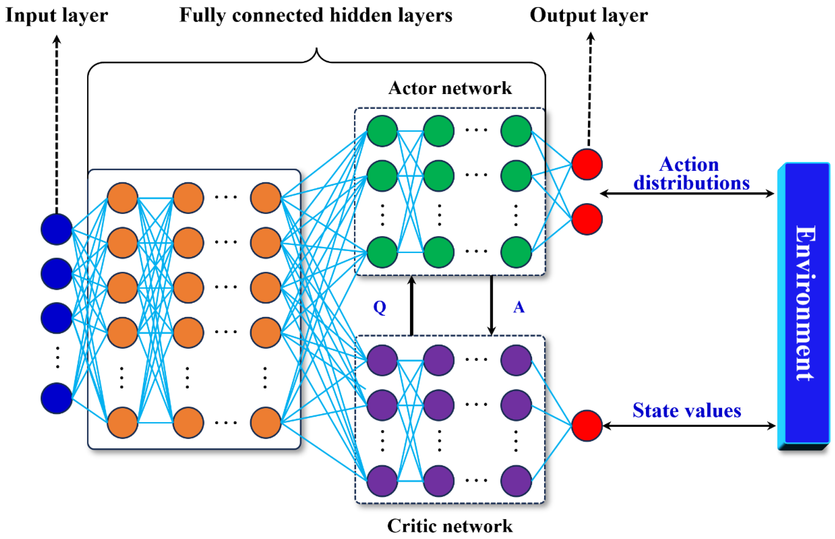
As shown in Figure 5, the Actor–Critic network is a reinforcement learning architecture that combines policy gradient and value function estimation, in which (1) the Actor network uses neural net π(a|s;θ) to approximate π(a|s), where θ is trainable parameters of the neural net, aiming to learn an optimal policy that maximizes the expected cumulative reward; (2) the Critic network uses neural net q(s,a,ω) to approximate Q_π(s,a), where ω is a trainable parameter of the neural net, aiming to compare the expected return from the selected actions with the actual rewards received and provide feedback to the Actor for policy improvement.

The training strategy of policy network uses the approximate policy gradient ${\nabla }_{\mathbf{\theta }}J(\mathit{\theta })$ to update the parameter θ. The unbiased estimation of the strategy gradient is described as follows

$$\widehat{g}(s,a;\mathit{\theta })\triangleq q(s,a;\mathit{\omega })\cdot {\nabla }_{\mathit{\theta }}\ln \pi (a|s;\mathit{\theta })$$

(25)

where q(s,a,ω) is the approximate of action-value function Q_π(s,a). Then, parameter θ of the policy neural network is updated by gradient ascent:

$$\mathit{\theta }\leftarrow \mathit{\theta }+\rho \cdot \widehat{g}(s,a;\mathit{\theta })$$

(26)

herein ρ is the learning rate of policy network.

Based on the above-mentioned update strategy, the Actor will gain higher score, which results in the dependence of critic network evaluation ability. The state-value function V_π(s) can be approximate to the following:

$$v(s;\mathit{\theta })=E_{A~\pi (\cdot |s;\mathit{\theta })}\left[q(s,A;\mathit{\omega })\right]$$

(27)

where v(s; θ) is the mean of Critic score.

At t-step, the output of value-state network is as follows:

$${\widehat{q}}_t=q(s_t,a_t;\mathit{\omega })$$

(28)

which is the estimation of the action-value function Q_π(s_t,a_t). At t + 1 step, the temporal-difference (TD) target is calculated with the observed r_t, s_t+1 and a_t+1, defined as follows:

$${\widehat{y}}_t\triangleq r_t+\gamma \cdot q(s_{t+1}.a_{t+1};\mathit{\omega })$$

(29)

which is also the estimation of the action-value function Q_π(s_t,a_t). However, the later estimation is closer to the truth due to the consideration of actual observed reward r_t. To update the parameters of value-state network, the loss function and its gradient are defined as follows:

$$\left\{\begin{array}{l}L(\mathit{\omega })\triangleq {\displaystyle \frac{1}{2}}{\left[q(s_t,a_t;\mathit{\omega })-{\widehat{y}}_t\right]}^2\\ {\nabla }_{\mathit{\omega }}L(\mathit{\omega })=\underset{\mathrm{TD} \mathrm{error} {\delta }_t}{\underbrace{({\widehat{q}}_t-{\widehat{y}}_t)}}\cdot {\nabla }_{\mathit{\omega }}q(s_t,a_t;\mathit{\omega })\end{array}\right.$$

(30)

then, conduct the next gradient descent to update ω:

$$\mathit{\omega }\leftarrow \mathit{\omega }+\alpha \cdot {\nabla }_{\mathit{\omega }}L(\mathit{\omega })$$

(31)

where α is the learning rate of value-state network.

The training process of Actor–Critic network is defined as follows:

Assume the current policy network parameters are θ_now and the value network parameters are ω_now, perform the following steps to update the parameters to θ_new and ω_new:

Step 1: Observe the current state s_t and make a decision based on the policy network: at~π(·|s_t; θ_now); then, let the agent perform the action a_t.

Step 2: Receive the reward rt and observe the next state s_t+1 from the environment.

Step 3: Make a decision based on the policy network: ${\tilde{a}}_{t+1}~\pi (\cdot |s_{t+1};{\theta }_{\mathrm{now}})$, but do not let the agent perform action ${\tilde{a}}_{t+1}$.

Step 4: Evaluate the value network:

$${\widehat{q}}_t=q(s_t,a_t;{\mathit{\omega }}_{\mathrm{now}}), {\widehat{q}}_{t+1}=q(s_{t+1},{\tilde{a}}_{t+1};{\mathit{\omega }}_{\mathrm{now}})$$

(32)

Step 5: Compute the TD target and TD error:

$${\widehat{y}}_t=r_t+\gamma \cdot {\widehat{q}}_{t+1}, {\delta }_t={\widehat{q}}_t-{\widehat{y}}_t$$

(33)

Step 6: Update the value network:

$${\mathit{\omega }}_{\mathrm{new}}\leftarrow {\mathit{\omega }}_{\mathrm{now}}-\alpha \cdot {\delta }_t\cdot {\nabla }_{w}q(s_t,a_t;{\mathit{\omega }}_{\mathrm{now}})$$

(34)

Step 7: Update the policy network:

$${\mathit{\theta }}_{\mathrm{new}}\leftarrow {\mathit{\theta }}_{\mathrm{now}}+\rho ·{\widehat{q}}_t·{\nabla }_{\mathit{\theta }}\ln \pi \left(a_t|s_t;{\mathit{\theta }}_{\mathrm{now}}\right)$$

(35)

3.3. The Framework of AC-Kriging-Based Structural Reliability Analysis

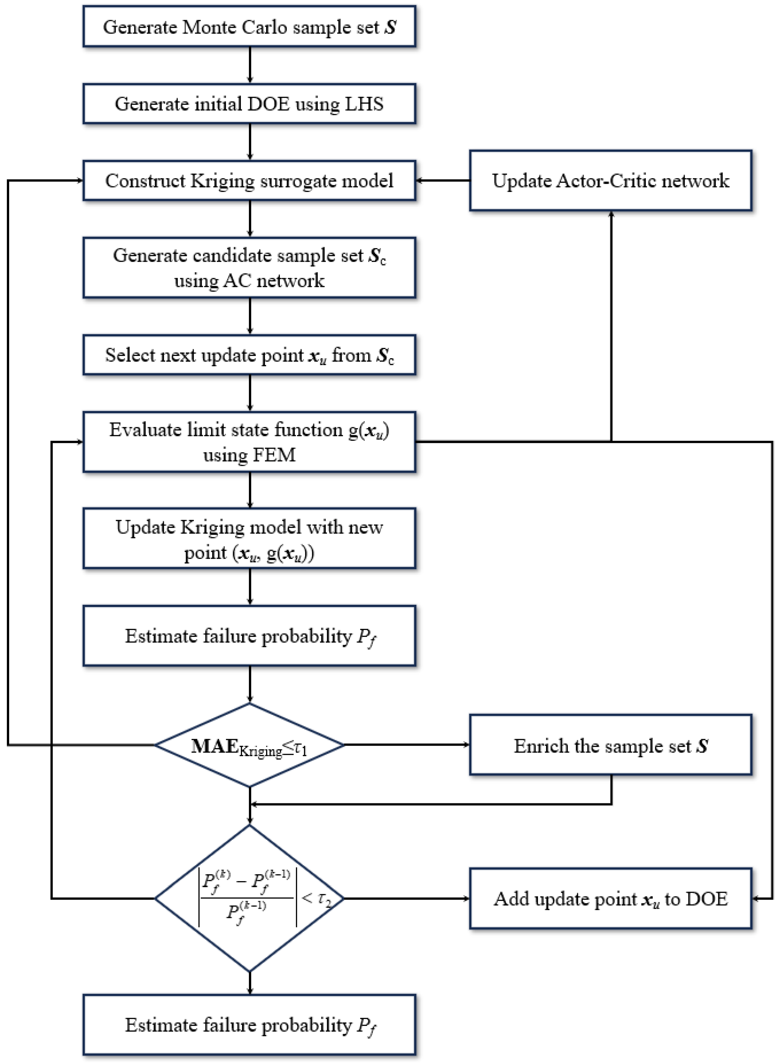
The proposed AC-Kriging method aims at introducing a novel active sampling and modeling framework for efficient and accuracy structural reliability analysis by integrating the DRL-based Actor–Critic network and the Kriging model. The detailed overview of the framework is illustrated in Figure 6. The computational implementation of the AC-Kriging framework is detailed in Algorithm 1, which systematically describes the integration of reinforcement-learning-based active sampling with Kriging surrogate modeling for efficient structural reliability analysis. In addition, the AC-Kriging framework operates through three distinct phases: initialization, iterative optimization through Actor–Critic network-guided sampling, and final structural reliability assessment.

Algorithm 1. Pseudocode of the AC-Kriging Method for Structural Reliability Analysis

1. Input: Design space $\mathbf{X}\subset {ℝ}^n$, initial sample size $m$, convergence tolerance $\tau$, reward weights of Actor-Critic network $a_1,a_2,a_3,a_4$.

2. Output: Failure probability $P_f$, reliability degree $R$.

3. Initialization Phase.

4. Generate initial samples using Latin Hypercube Sampling: $X_0=\{x_1,x_2,\dots ,x_m\}$;

5. Evaluate limit state function: $G_0=\{g(x_1),g(x_2),\dots ,g(x_m)\}$;

6. Build initial Kriging model with samples $(X_0,G_0)$;

7.  Compute correlation matrix $\mathbf{R}$ with parameters $\alpha =\{{\alpha }_1,{\alpha }_2,\dots ,{\alpha }_n\}$;

8.  Estimate regression coefficients: $\widehat{\beta }={(F^T{R}^{-1}F)}^{-1}{F}^T{R}^{-1}{G}_0$;

9.  Estimate process variance: ${\widehat{\sigma }}^2={(G_0-F\widehat{\beta })}^T{R}^{-1}(G_0-F\widehat{\beta })/m$;

10. Initialize Actor network parameters ${\theta }_0$ and Critic network parameters ${\omega }_0$;

11. Randomly select starting point: $x_k\in X_0$, set iteration counter $k=1$.

12. Main Iteration Loop.

13. While convergence criteria not satisfied Do

14.  Construct state $s_k$ based on current position $x_k$ and Kriging: $s_k=[x_k,\widehat{g}(x_k),{\sigma }_{\widehat{g}}^2(x_k)]$; 15.   Generate displacement action using Actor network: $a_k~\pi (\cdot |s_k;{\theta }_k)$;

16.   Compute new sample point location: $x_{k+1}=x_k+a_k$ (ensure within design space); 17.   Evaluate limit state function: $g_{k+1}=\widehat{g}(x_{k+1})$;

18.   Update sample sets: $X\leftarrow X\cup \left\{x_{k+1}\right\}$,$G\leftarrow G\cup \left\{g_{k+1}\right\}$.

19.  Update Kriging model parameters.

20.   Update correlation matrix $R$ and correlation parameters $\mathbf{\alpha }$;

21.   Recompute regression coefficients $\widehat{\beta }$ and process variance ${\widehat{\sigma }}^2$.

22.  Calculate reward $R_k$ based on multiple criteria:

23.   $r_{edge}=\exp (-|g_{k+1}|)$ (boundary proximity reward);

24.   $r_{movement}=\exp (-|g_{k+1}-g_{last}|)$ if $|\mathrm{g}\_\{\mathrm{k}+1\left\}\right| < 0.5$, else 0;

25.   $r_{exploration}=\mathrm{constant}$ if distance to boundary $> 0.3$, else 0;

26.   $r_{keep}=\max (0,0.5-|g_{k+1}|)$ if $\left|g_{k+1}\right|<0.5$, else 0;

27.   $R_k=a_1\cdot r_{edge}+a_2\cdot r_{movement}+a_3\cdot r_{exploration}+a_4\cdot r_{keep}$.

28.  Update Actor-Critic networks.

29.   Update Critic network: ${\omega }_{k+1}\leftarrow {\omega }_k-\rho {\nabla }_{\omega }L({\omega }_k)$;

30.   Update Actor network: ${\theta }_{k+1}\leftarrow {\theta }_k+\eta {\nabla }_{\theta }J({\theta }_k)$.

31.  Check and Update.

32.   Criteria 1: Kriging model convergence $MA{E}_{Kriging}<{\tau }_1$; 33.   Criteria 2: Failure probability convergence $\left|{\displaystyle \frac{P_{f,k}-P_{f,k+1}}{P_{f,k+1}}}\right|<{\tau }_2$

34.   Update: $x_k\leftarrow x_{k+1}$, $k\leftarrow k+1$.

35.  End While

36. Structural Reliability Analysis.

37. Generate $N$ samples based on Monte Carlo: $X_{MC}=\{x_1,x_2,\dots ,x_N\}$;

38. Count failures: $N_f={\displaystyle \sum _{i=1}^{N}I}[g(X)\le 0]$;

39. Calculate failure probability: $P_f=N_f/N$

40. Return $P_f$

3.3.1. Initialization

The initialization phase establishes the computational foundation for the AC-Kriging method by creating both the initial Kriging surrogate model and the reinforcement learning environment. This phase begins with the generation of initial design points using Latin Hypercube Sampling (LHS) to ensure uniform coverage across the n-dimensional design space. The LHS approach generates m initial sample points X₀ = {x₁, x₂, …, x_m}, where each point represents a realization of the random variables in the structural reliability problem.

Following sample generation, the limit state function g(x_i) is evaluated at each initial sample point through high-fidelity finite element analysis or other appropriate computational methods. These evaluations yield the response dataset G₀ = {g(x₁), g(x₂), …, g(x_m)}, which forms the basis for constructing the initial Kriging surrogate model.

The initial Kriging model construction involves the estimation of three critical parameter sets. First, the correlation matrix R is computed, along with the correlation parameters α = {α₁, α₂, …, α_n}, which control the spatial correlation structure of the Gaussian process. Second, the regression coefficients and process variance are estimated by Equation (20). The initialization concludes by establishing the reinforcement learning components. The Actor network parameters θ₀ and Critic network parameters ω₀ are randomly initialized, creating the foundation for the subsequent active learning process. One starting point x_k is randomly selected from the initial sample set X₀, which serves as the agent’s initial position. The iteration counter k is set to 1, marking the beginning of the iterative optimization phase.

3.3.2. Actor–Critic Network-Based Active Sampling and Kriging Modeling Method

The iterative optimization phase represents the core innovation of the AC-Kriging method. This phase operates through a continuous feedback loop between the Actor–Critic networks and the evolving Kriging surrogate model, with each iteration strategically selecting new sample points to maximize information gain for reliability analysis. The details are defined as follows:

Step 1: Each iteration begins with state construction, where the current system state s_k is formulated based on the agent’s current position x_k and the Kriging model’s predictions. The state vector s_k = [x_k, ĝ(x_k), σ²ĝ(x_k), boundary proximity] encapsulates essential information including the current location, the Kriging model’s prediction at that location, the associated prediction uncertainty, and proximity indicators to the limit state boundary. This comprehensive state representation enables the Actor network to make informed decisions about the next sample.

Step 2: The Actor network processes the state information to generate a displacement action a_k~π(·|s_k; θ_k), which represents the optimal direction and magnitude for moving to the next sample point. The action space is designed as a continuous domain, allowing for precise positioning of sample points anywhere within the feasible design space. The new sample point location is then computed using x_k+1 = x_k + a_k, with appropriate boundary constraints to ensure the new point remains within the design space.

Step 3: The newly selected sample point undergoes evaluation, where the true limit state function g(x_k+1) is computed through high-fidelity analysis. This new information is incorporated into the sample database by updating both the sample set X_k+1 = X_k ∪ x_k+1 and the response set G_k+1 = G_k ∪ g_k+1.

Step 4: The Kriging model update process ensures that the surrogate model continuously improves its approximation of the limit state function. The correlation matrix R and correlation parameters α are updated to accommodate the new sample point, followed by recomputation of the regression coefficients $\widehat{\beta }$ and process variance ${\widehat{\sigma }}^2$. This incremental update strategy maintains computational efficiency while ensuring model accuracy.

Step 5: The Actor–Critic network updates employ temporal difference learning for the Critic network by Equation (31) and policy gradient methods for the Actor network by Equation (26). These updates enable the networks to learn optimal sampling strategies specific to the current reliability problem.

Step 6: During the iterative process, dual convergence criteria are continuously monitored. The first criterion evaluates Kriging model precision by checking whether the maximum prediction uncertainty falls below the threshold ε_m. The second criterion assesses the stability of failure probability estimates by monitoring the relative change between successive iterations. The iteration completes by updating the agent’s position (x_k ← x_k+1) and incrementing the iteration counter, preparing for the next cycle of the optimization process.

3.3.3. Structural Reliability Analysis

The sample points selected through the AC-Kriging method are utilized to construct the Kriging model for structural reliability analysis. The training process follows standard procedures with samples divided into training and validation sets. During the iterative optimization phase, the process monitors dual convergence criteria.

The first criterion is the mean absolute error (MAE) focusing on Kriging model precision, which is defined as follows:

$$\mathbf{M}\mathbf{A}{\mathbf{E}}_{\mathrm{Kriging}}={\displaystyle \frac{1}{n}}{\displaystyle \sum _{i=1}^n\left|y_i-{\widehat{y}}_i\right|}<{\tau }_1$$

(36)

where n is the number of test samples; τ₁ is the first criteria of convergence; y_i is the i-th true output of Kriging model; and ${\widehat{y}}_i$ is the i-th prediction output of Kriging model. Then, the coefficient of variation (COV) of the failure probability estimation of the Kriging model is calculated to evaluate the convergence of the reliability analysis:

$$\mathrm{COV}({\widehat{P}}_f)=\sqrt{\left(1-{\widehat{P}}_f\right)/N\cdot {\widehat{P}}_f}$$

(37)

where N is the number of samples based on MCS. Finally, the trained Kriging model is applied to structural reliability assessment.

Subsequently, the convergence of the prediction accuracy based on the pre-determined number of iterations or the surrogate model, which can be defined as follows:

$$\left|{\displaystyle \frac{P_f^{(k)}-P_f^{(k-1)}}{P_f^{(k-1)}}}\right|<{\tau }_2$$

(38)

where P_f^(k) is the t-step failure probability estimate, and τ₂ is the convergence threshold of criteria 2. In this study, τ₁ and τ₂ are equal to 0.05 and 0.01, respectively.

4. Case Studies

In this section, three cases are studied to validate the AC-Kriging method. The first case involves a series system with four failure modes. The second case examines a two-degree-of-freedom dynamic system. The third case analyzes the deformation reliability analysis of turbine blade. Four active sampling methods are selected for comparison with AC-Kriging: IS [11], DS [12], SS [13], Kriging with expected improvement infill sampling (Kriging-EI) [47], and an active sampling method combining Kriging and MCS (AK-MCS) [48].

4.1. Nonlinear Series System Reliability Analysis

This case is a two-dimensional reliability assessment problem with four failure modes [49,50]. The LSF is described as follows:

$$g(x_1,x_2)=\min \left\{\begin{array}{l}\left(x_1-x_2\right)+{\displaystyle \frac{k}{\sqrt{2}}};3+0.1{\left(x_1-x_2\right)}^2-{\displaystyle \frac{\left(x_1+x_2\right)}{\sqrt{2}}}\\ \left(x_2-x_1\right)+{\displaystyle \frac{k}{\sqrt{2}}};3+0.1{\left(x_1-x_2\right)}^2-{\displaystyle \frac{\left(x_1+x_2\right)}{\sqrt{2}}}\end{array}\right\}$$

(39)

where k is a constant equal to 7. The random variables x₁ and x₂ are normally distributed and their statistical characteristics are shown in

Table 1. The distribution of random variables in Case 1.

Parameter	Lower Bound	Upper Bound	Mean	Standard Deviation	Distribution
x1	−6	6	0	1	Normal
x2	−6	6	0	1	Normal

.

To obtain the number of samples, N is calculated based on Equation (37), which gives a failure probability of 10⁻³ and COV < 5%. The minimum required sample size is determined as N > (1 − 10⁻³)/(0.025 × 10⁻³) = 399,600. To establish a reference solution, direct MCS is performed with 5 × 10⁵ samples to obtain the benchmark failure probability. Various active sampling methods are employed to construct surrogate models, which are then used with MCS to estimate the failure probability and evaluate the efficiency of different methods. The relative error ε_r compared with direct MCS is defined as follows:

$${\epsilon }_r=\left|{\displaystyle \frac{{\widehat{P}}_f-P_{f,MCS}}{{\widehat{P}}_f}}\right|$$

(40)

where P_f,MCS is the true failure probability base on direct MCS.

To establish the reference solution for comparison, a Monte Carlo convergence study is conducted, as shown in

Table 2. MCS study for Case 1: nonlinear series system.

Samples	103	104	105	2.5 × 105	5 × 105	106
Pf	1.000 × 10−3	2.440 × 10−3	2.250 × 10−3	2.250 × 10−3	2.316 × 10−3	2.308 × 10−3

. The failure probability estimates exhibit significant variation at smaller sample sizes (1.000 × 10⁻³ at 10³ samples, 2.440 × 10⁻³ at 10⁴ samples) and gradually stabilize as the sample size increases. The estimate stabilizes at 2.316 × 10⁻³ for 5 × 10⁵ samples and remains at 2.308 × 10⁻³ with 10⁶ samples; therefore, the failure probability obtained from 5 × 10⁵ samples is taken as the converged value.

Figure 7 shows the true limit state surface of Case 1. The comparison of sampling point distributions among different methods using the same number of experimental points is shown in Figure 8. The blue points represent samples in the failure domain, while the red points represent samples in the safe domain. It can be observed that traditional methods such as IS, DS, and SS tend to distribute points more uniformly across the entire design space. In addition, the Kriging-EI method shows some adaptive behavior by placing more samples near the boundary compared to traditional methods but still maintains a relatively scattered distribution across the design space. In contrast, the proposed AC-Kriging method demonstrates superior adaptive sampling by concentrating points strategically along the LSF boundary. This targeted strategy enables more accurate LSF approximation with the same computational budget, achieving a better classification of safe and failure domains.

Table 3. Performance comparison of different active sampling methods in Case 1.

Method	N (Number of Samples)	Pf	εr (%)
Direct MCS	5 × 105 (COV(Pf) = 2.9%)	2.316 × 10−3	-
IS	3562	2.092 × 10−3	10.71
DS	2219	2.203 × 10−3	5.13
SS	2.8 × 104	2.225 × 10−3	4.09
Kriging-EI	156	2.180 × 10−3	6.24
AK-MCS	96	2.233 × 10−3	3.72
AC-Kriging	52	2.296 × 10−3	0.87

presents the performance comparison of different active sampling methods for failure probability estimation. Using direct MCS as the reference (5 × 10⁵ samples, P_f = 2.316 × 10⁻³), the proposed AC-Kriging achieves superior efficiency with only 52 samples and a 0.87% relative error. Other methods require significantly more samples: AK-MCS (96 samples, 3.72% error), Kriging-EI (156 samples, 6.24% error), DS (2219 samples, 5.13% error), IS (3562 samples, 10.71% error), and SS (2.8 × 10⁴ samples, 4.09% error). The results clearly demonstrate that AC-Kriging achieves the highest computational efficiency while maintaining excellent accuracy in failure probability evaluation.

4.2. A Two-Degree-of-Freedom Dynamic System

As shown in Figure 9, a two-degree-of-freedom dynamic system is considered using the LSF computed by the force capacity (F_s) of the stiffness of second spring (K_s), which is defined below [49].

$$g(M_p,M_s,K_p,K_s,{\xi }_p,{\xi }_c,S_0,F_s)=F_s-3K_s\times {\left({\displaystyle \frac{\pi S_0}{4{\xi }_s{\omega }_s}}\left[{\displaystyle \frac{{\xi }_a{\xi }_s}{{\xi }_p{\xi }_s\left(4{\xi }_a^2+{\theta }^2\right)+\gamma {\xi }_a^2}}\times {\displaystyle \frac{\left({\xi }_p{\omega }_p^3+{\xi }_s{\omega }_s^3\right){\omega }_p}{4{\xi }_a{\omega }_a^4}}\right]\right)}^{1/2}$$

(41)

where γ represents the mass ratio M_s/M_p, ω_n denotes the natural frequency calculated as (ω_p + ω_s)/2, ξ_n indicates the damping coefficient given by (ξ_p + ξ_s)/2, θ signifies the frequency ratio (ω_p − ω_c)/ω_n, and S₀ represents the white noise intensity. The stochastic parameters follow log-normal probability distributions, with their statistical characteristics detailed in

Table 4. The distribution of random variables in Case 2.

Parameter	Lower Bound	Upper Bound	Mean	Standard Deviation	Distribution
Mp	0.9	1.1	1	0.1	logNormal
Ms	0.009	0.011	0.01	0.001	logNormal
Kp	0.8	1.2	1	0.2	logNormal
Ks	0.00998	0.0102	0.01	0.002	logNormal
ξp	0.03	0.07	0.05	0.02	logNormal
ξc	0.01	0.03	0.02	0.01	logNormal
S0	90	110	100	10	logNormal
Fs	13.5	16.5	15	1.5	logNormal

.

To establish the reference solution for comparison, a Monte Carlo convergence study is conducted, as shown in

Table 5. MCS study for Case 2: A two degree of freedom dynamic system.

Samples	103	104	105	2.5 × 105	5 × 105	106
Pf	2.572 × 10−2	2.788 × 10−2	3.014 × 10−2	3.245 × 10−2	3.164 × 10−2	3.216 × 10−2

. The failure probability estimates exhibit significant variation at smaller sample sizes (2.572 × 10⁻² at 10³ samples, 3.245 × 10⁻² at 2.5 × 10⁵ samples) and gradually stabilize as the sample size increases. The estimate converges to 3.164 × 10⁻² at 5 × 10⁵ samples and remains consistent at 3.216 × 10⁻² with 10⁶ samples, confirming that 5 × 10⁵ samples provide a reliable reference solution with sufficient convergence for this problem.

Table 6. Performance comparison of different active sampling methods in Case 2.

Method	N (Number of Samples)	Pf	εr (%)
Direct MCS	5 × 105 (COV(Pf) = 2.9%)	3.164 × 10−2	-
IS	4636	2.589 × 10−2	22.21
DS	3534	2.732 × 10−2	15.81
SS	3.352 × 104	2.956 × 10−2	7.04
Kriging-EI	264	2.863 × 10−2	10.51
AK-MCS	172	3.374 × 10−2	6.22
AC-Kriging	101	3.098 × 10−2	2.13

presents the performance comparison of different active sampling methods for failure probability estimation in Case 2. Using direct MCS as the reference (5 × 10⁵ samples, P_f = 3.164 × 10⁻²), the proposed AC-Kriging method achieves superior efficiency with only 101 samples and 2.13% relative error. Other methods require significantly more samples: AK-MCS (172 samples, 6.22% error), Kriging-EI (264 samples, 10.51% error), DS (3534 samples, 15.81% error), SS (3.352 × 10⁴ samples, 7.04% error), and IS (4636 samples, 22.21% error). The results demonstrate that AC-Kriging achieves the highest computational efficiency while maintaining excellent accuracy in failure probability evaluation.

4.3. Radial Deformation Reliability Analysis of Aeroengine Turbine Blade

To assess the robustness of AC-Kriging in practical engineering scenarios, this research examines the reliability analysis of maximum radial displacement for an aeroengine’s high-pressure turbine blade. The structural reliability is determined by comparing the blade’s radial deformation with its allowable deformation threshold, with a detailed analysis provided in [1]. Figure 10a illustrates the blade’s geometric configuration and applied boundary conditions, and Figure 10b shows the finite element model of turbine blade.

In this case, the turbine blade root remains constrained while accounting for centrifugal acceleration effects arising from high-speed rotation. The finite element model of the turbine blade consists of 26,735 nodes and 7557 elements. The selected material is K417 with a density of 8210 kg/m³, an elastic modulus of 2.15 × 10⁵ MPa, and a Poisson’s ratio of 0.28. Five distinct convective heat transfer boundary conditions are applied to the root, lower section, middle section, upper section, and blade tip regions. These boundary conditions are characterized by four sets of convection parameters: temperatures T₁, T₂, T₃, T₄ and corresponding heat transfer coefficients a₁, a₂, a₃, a₄. Nine stochastic variables follow normal distribution patterns, as detailed in

Table 7. The distribution of random variables in Case 3.

Parameter	Lower Bound	Upper Bound	Mean	Standard Deviation	Distribution
ω(rad/s)	1062.88	1273.12	1168	35.04	Normal
T1(°C)	937.0	1123.0	1030	31.00	Normal
T2(°C)	891.8	1068.2	980	29.40	Normal
T3(°C)	746.2	893.8	820	24.60	Normal
T4(°C)	491.4	588.6	540	16.20	Normal
α1 (Wm−2K−1)	10,697.96	12,814.04	11,756	352.68	Normal
α2 (Wm−2K−1)	7513.23	8992.77	8253	246.59	Normal
α3 (Wm−2K−1)	5957.77	7136.23	6547	196.41	Normal
α4 (Wm−2K−1)	2848.3	3411.7	3130	93.90	Normal

, where indices 1–4 represent the progression from exterior to interior surfaces. Finite element simulations are conducted under these prescribed boundary conditions, with the results presented in Figure 11 as baseline data for a subsequent reliability assessment.

For this case, the LSF is given as follows:

$$g\left(X\right)=u_0-u_{\max }\left(X\right)$$

(42)

where u₀ represents the allowable radial displacement of 1.40 mm, u_max(X) denotes the peak radial displacement obtained from finite element analysis, and X is the input random parameters including ω, T₁, T₂, T₃, T₄, a₁, a₂, a₃, and a₄.

Figure 12 demonstrates that the reliability degree rapidly converges to approximately 0.9968 within the first 10⁴ samples and remains stable thereafter.

To establish the reference solution for comparison, a Monte Carlo convergence study is conducted, as shown in

Table 8. MCS study for Case 3: Radial deformation reliability analysis of aeroengine turbine blade.

Samples	102	103	3 × 103	8 × 103	1 × 104	5 × 104	1.5 × 105
Pf	1 × 10−2	0.5 × 10−2	0.68 × 10−2	0.36 × 10−2	0.32 × 10−2	0.33 × 10−2	0.31 × 10−2

. The failure probability estimates exhibit significant variation at smaller sample sizes (1 × 10⁻² at 10³ samples, 0.68 × 10⁻² at 3 × 10³ samples) and gradually stabilize as the sample size increases. The estimate converges to 0.31 × 10⁻² at 1.5 × 10⁵ samples and remains consistent at 0.33 × 10⁻² with 5 × 10⁴ samples, confirming that 1.5 × 10⁵ samples provide a reliable reference solution with sufficient convergence for this problem.

Table 9. Probability distribution of a random input variable.

Method	N (Number of Samples)	Pf	εr (%)
Direct MCS	1.5 × 105 (COV(Pf) = 4.63%)	3.10 × 10−3	-
IS	6894	2.23 × 10−3	39.01
DS	4552	2.38 × 10−3	30.25
SS	4.2 × 104	2.49 × 10−3	24.50
Kriging-EI	421	2.42 × 10−3	27.94
AK-MCS	283	2.68 × 10−3	15.67
AC-Kriging	147	2.89 × 10−3	7.27

compares the computational efficiency of six probability estimation methods for the turbine blade reliability analysis. The results show that while Direct MCS requires 1.5 × 10⁵ samples to achieve a failure probability of 3.10 × 10⁻³, advanced sampling techniques significantly reduce the computational costs. AC-Kriging demonstrates the highest efficiency with only 147 samples and a 7.27% relative error, followed by AK-MCS requiring 283 samples with 15.67% error, and Kriging-EI with 421 samples and 27.94% error. Traditional methods require substantially more samples: DS (4552 samples, 30.25% error), SS (4.2 × 10⁴ samples, 24.50% error), and IS (6894 samples, 39.01% error). The results demonstrate that AC-Kriging achieves the highest computational efficiency and accuracy in the complex structural reliability analysis of turbine blade.

AC-Kriging achieves higher efficiency by replacing uniform sampling with a targeted search that concentrates evaluations near the limit state surface. Traditional methods are inefficient because they search the whole design space evenly, while the critical g(x) ≈ 0 region is small. For failure probabilities on the order of 10⁻³, approximately 99.9 % of uniformly drawn samples lie in the safe domain and contribute little to the estimate. AC-Kriging overcomes this limitation based on the Actor–Critic network, where the reward function (Equations (12)–(16)) drives the agent toward high-score regions, ensures exploration with a little computational cost, and maintains consistent boundary tracking. The temporal difference learning mechanism provides continuous feedback to refine sampling strategies, unlike static learning functions that cannot adapt to problem-specific characteristics. The continuous state–action representation enables precise boundary following with adaptive step sizes based on local LSF curvature, scaling linearly with dimension rather than exponentially. Therefore, the AC-Kriging method can reduce the computational cost by a factor of 10²–10³ and maintain the high precision of reliability analysis.

5. Conclusions

This paper proposes an Actor–Critic network-enhanced Kriging method (AC-Kriging) for efficient structural reliability analysis of aeroengine components by integrating deep reinforcement learning with adaptive surrogate modeling. The main conclusions are drawn as follows:

(1)

AC-Kriging demonstrates superior sampling efficiency compared to conventional methods, achieving comparable accuracy with only 52–147 samples versus the thousands required by traditional methods like IS, DS, and SS while maintaining relative errors below 8%.

(2)

The Actor–Critic framework effectively optimizes sampling strategies through intelligent reward function design, which concentrates sampling in reliability-critical boundary regions and achieves adaptive sequential decision-making rather than uniform space-filling.

(3)

The continuous state–action representation enables precise boundary following with adaptive step sizes, scaling linearly with dimension and addressing the curse of dimensionality that limits traditional approaches in high-dimensional problems.

(4)

Case studies validate AC-Kriging’s effectiveness across diverse applications, from nonlinear systems to practical turbine blade reliability assessment, with dual convergence criteria ensuring both model precision and algorithmic stability.

(5)

The method successfully balances exploration and exploitation through its reinforcement learning framework, enabling effective handling of complex aerospace engineering problems with non-convex, multi-modal failure boundaries.

The current study only considers steady-state conditions and does not address the added complexity of time-varying environmental loads or component degradation. Future research could focus on extending AC-Kriging to time-dependent reliability problems and investigating its applicability in real-time reliability assessment scenarios for safety-critical aerospace systems.