Adaptive Global Predefined-Time Control Method of Aerospace Aircraft

Abstract

This paper proposes a global, predefined time control method based on a predefined time disturbance observer to address the issues of wide flight airspace, large aerodynamic deviations, and high precision requirements for the entire process of aerospace aircraft re-entry. Firstly, this method proposes an adjustable predefined time nonsingular sliding mode disturbance observer, which can not only accurately estimate the modeling uncertainty and external aerodynamic disturbances of the aerospace aircraft, but also quickly converge while suppressing chattering. Then, based on the disturbance observation results, combined with a new performance function and nonsingular predefined-time sliding mode, a global predefined-time controller suitable for any order system was designed. Unlike existing methods that can only ensure that the initial deviation converges to the deviation boundary within a predefined time and then remains within the deviation boundary, it can ensure that any deviation generated within the error boundary also converges within the predefined time. Finally, the effectiveness and superiority of the proposed control scheme were verified through comparative simulation.

1. Introduction

Aerospace aircraft highly integrate aviation technology with aerospace technology, and their reusable characteristics can effectively reduce transportation costs [1]. The space shuttle of NASA (WA, USA) [2] was one of the earliest aerospace aircraft used for flight. Subsequently, NASA developed the X-37B [3] and operated it in orbit for a long time until the recent fourth space flight of SpaceX’s starship (CA, USA), which pushed the attention of the aerospace aircraft to its peak. The dynamic model of aerospace aircraft has the characteristics of strong coupling, rapid state change, and strong parameter uncertainty [4,5], which puts forward high stability, fast response, and anti-interference requirements for attitude control of aerospace aircraft, and has attracted more and more attention from scholars. Compared to robust control methods [6], the control method based on error observer can effectively reduce high-gain phenomena. Therefore, this paper adopts a controller design scheme based on error observer.

Due to the significant differences in flight environment and status of aerospace aircraft, external disturbances and parameter uncertainties always have an impact on attitude control. In order to reduce the impact of disturbances and parameter uncertainties, scholars have conducted extensive research on disturbance compensation schemes based on disturbance observers [7,8,9,10,11]. Bai(2017) [12] used a nonlinear extended observer for adaptive tracking compensation of spacecraft attitude. Song (2024) [13] used a finite-time disturbance observer to compensate for spacecraft disturbances and achieve robust attitude control problems. Zhang (2023) [14] proposed a fixed-time neural network disturbance observer for disturbance compensation in spacecraft rendezvous and docking control. The above paper only guarantees finite= or fixed-time convergence of observation errors, and there is currently limited research on observers with predefined-time convergence. Recently, refs. [15,16], respectively, proposed predefined-time disturbance observers for spacecraft applications, but neither considered the servo model and only observed disturbances in the second-order rigid body model of the spacecraft.

For the predefined-time attitude control problem of aerospace aircraft, Eliker (2020) [17] designed a finite-time-adaptive fast terminal sliding mode to ensure the control system is finite-time stable against disturbances, and the tracking error can converge to a small neighborhood of the origin. Reference [18] designed a continuous finite-time high-order sliding mode controller and used a nonlinear disturbance observer to estimate uncertainties, achieving disturbance suppression. However, the convergence time of finite-time sliding mode control methods is related to the initial state. To make the system state convergence time independent of the initial values and avoid excessive control input caused by control singularity, Reference [19] proposed a nonsingular fixed-time sliding mode control method based on a fixed-time extended state observer and analyzed the system stability based on Lyapunov theory. Reference [20] designed a nonsingular fixed-time terminal sliding mode controller for the attitude control problem of reusable vehicles, and the simulation results show that the guidance commands can be accurately tracked within a fixed time in the presence of model uncertainties and external disturbances. Although the convergence time of fixed-time sliding mode control is independent of the initial state, the upper bound of the convergence time needs to be obtained through complex calculations and cannot be explicitly included in the controller. To enable the upper bound of the system convergence time to be set via a single parameter at the initial design stage, Sanchez-Torres (2015) [21] proposed a predefined-time control method. JU (2022) [22] proposed a predefined-time fractional order sliding mode control method incorporating a high-order predefined-time extended state observer, making the system convergence time explicitly contained in the controller. Finally, it is ensured that the time for the attitude tracking error to reach the sliding mode surface and for the sliding mode surface to converge to a small neighborhood of the origin can be set via a single parameter.

The robustness and stability of the aircraft attitude control system can be well satisfied by the various above-mentioned control methods. However, these methods largely depend on the design form of the control law and the selection of its parameters, and it is difficult to ensure quantitative regulation of their dynamic responses. The flight environment during the re-entry process of the aerospace aircraft is harsh, and the dynamic quality of its control system also has a great impact on flight stability control. Therefore, when designing the controller, it is also necessary to consider the influence of the transient process of the attitude tracking error on the control system. Preset performance control can perform quantitative regulation on the entire control process, and the transient and steady-state performance of the system during the control process (maximum overshoot, minimum convergence speed, and maximum steady-state error) can be characterized by a performance envelope function.

In recent years, predefined performance control laws have been fully developed: ref. [23] designed an adaptive predefined-time sliding mode predefined performance controller to address the attitude control problem of spacecraft under actuator failure conditions by combining a novel performance function with a nonsingular predefined-time sliding mode manifold. This controller can constrain the tracking error of the spacecraft within a predefined region within a predefined time, but it is only applicable to second-order systems and cannot fully converge to exact values. References [24,25] proposed constructing time-varying functions based on time-base generators to design predefined-time controllers, where the system converges to the origin within a required time. The convergence time can be set as an adjustable parameter of the controller and is independent of the initial conditions. On this basis, ref. [26] constructed two auxiliary functions based on time-varying functions and a corresponding predefined performance function to ensure that the attitude control deviation of the vehicle remains within the predefined performance function. However, time-varying functions may generate large gains, leading to excessive amplitudes of control variables and adversely affecting control performance. Reference [27] derived a finite-time adaptive state feedback fuzzy tracking controller based on predefined performance control, where the tracking error converges to a specified range within a finite time interval, with the maximum error not exceeding the boundary of the predefined performance function. Reference [28] further improved the predefined performance function in [27] to make it differentiable of any order, enhancing compatibility with high-order systems and avoiding high-gain control issues. Since performance functions only specify predefined convergence regions, such methods can only guarantee convergence to these regions within predefined times, without ensuring further convergence to predetermined values within the regions.

In summary, compared to previous studies by scholars, this paper has the following innovative points:

• Based on an adjustable predefined inequality condition, a nonsingular sliding mode observer with adjustable predefined-time is designed, which not only solves the singularity problem but also ensures that the disturbance boundary is independent of the observer parameters.
• A novel predefined-time controller is designed by combining novel performance function and nonsingular predefined-time sliding modes.
• The controller designed in this paper can not only ensure that the initial tracking error converges within the predefined time, but also ensures that any errors generated within the error boundary during the subsequent control process can converge within the predefined time.

The remaining part of this paper is as follows: Section 2 presents the control model of the aerospace aircraft and the first-order servo model, as well as feedback linearization. Section 3 designs a nonsingular sliding mode observer with adjustable predefined-time and a novel arbitrary globally order predefined-time controller. Section 4 demonstrates the advantages of our method through comparative simulation verification. Finally, Section 5 summarizes the content of the paper.

2. Preliminaries and Problem Formulation

In this section, we first present the required theorem and lemma, then introduce the aerospace aircraft model and feedback linearization.

2.1. Preliminaries

Consider the system as follows:

$$\dot{x}=f\left(x\right),x\left(0\right)=x_0$$

(1)

Theorem 1

([29]). A non-empty set $M\subset {ℝ}^n$ is said to be globally fixed-time attractive for system (1) if any solution $x\left(t,x_0\right)$ of (1) reaches $M$ in some finite time $t=t_0+T\left(x_0\right)$, where the settling-time function $T\left(x_0\right)$ is bounded by some positive number $T_m$, $i.e.$, $T\left(x_0\right)\le T_m$ for all $x_0\in {ℝ}^n$.

Definition 1

([30]). If the equilibrium point of the system (1) is the stable in a finite time, and the convergence time $T\left(x_0,\mu \right):R^n\to R$ satisfies: $T\left(x_0,\mu \right)\le T_c\forall x_0\in R^n$, then the equilibrium point of the system (1) is considered to be tunable predefined-time stable and $T_c$ is a predefined time. $\mu$ represents a tunable parameter.

Lemma 1

([30]). For the system (1), if there is a Lyapunov function $V\left(x\right)$, it satisfies the following conditions:

$$\dot{V}\le -{\displaystyle \frac{\pi }{\eta T_c\mu \sqrt{mn}}}\left(m{V}^{1-{\displaystyle \frac{\eta }{2}}}+{\mu }^{2}n{V}^{1+{\displaystyle \frac{\eta }{2}}}+2\mu \sqrt{mn}V\right)$$

(2)

then the system is tunable predefined-time stable. $T_c>0$ is the predefined-time, $m,n>0$, $0<\eta <1$, and $\mu >0$.

Compared with [31], the above adjustable predefined-time stability conditions add two adjustable parameters $m,n$, giving it greater degrees of freedom to adjust and making the actual convergence time closer to $T_c$.

Lemma 2

([32]). If $x_i\ge 0\left(i=1,2,\dots ,n\right)$ and $\gamma >0$, then the following inequalities hold:

$$\left\{\begin{array}{l}{\displaystyle \sum _{i=1}^n{x}_i^{\gamma }}\ge {\left({\displaystyle \sum _{i=1}^n{x}_i}\right)}^{\gamma },if0<\gamma <1\hfill \\ {\displaystyle \sum _{i=1}^n{x}_i^{\gamma }}\ge n^{1-\gamma }{\left({\displaystyle \sum _{i=1}^n{x}_i}\right)}^{\gamma },if\gamma >1\hfill \end{array}\right.$$

(3)

2.2. Attitude Control Model for Aerospace Aircraft

The kinematic and dynamic models of aerospace aircraft are as follows:

$$\begin{array}{l}\dot{\sigma }=G\left(\sigma \right)\omega \\ J\dot{\omega }=-\omega \times J\omega +M_c+M_d\end{array}$$

(4)

where $\sigma ={\left[\begin{array}{ccc}\alpha & \beta & \sigma \end{array}\right]}^{\mathrm{T}}$ is the attitude angle, $\omega ={\left[\begin{array}{ccc}{\omega }_x& {\omega }_y& {\omega }_z\end{array}\right]}^{\mathrm{T}}$ is the attitude angular velocity, $G\left(\sigma \right)\in {ℝ}^{3\times 3}$ is the state space matrix, $J\in {ℝ}^{3\times 3}$ is the inertia matrix of the space shuttle, $M_c\in {ℝ}^{3\times 1}$ is the control torque, and $M_d\in {ℝ}^{3\times 1}$ is the external additional moment interference. The form of $G\left(\sigma \right)$ and $J$ are provided in the Appendix A.

The expression for the control torque is

$$M_c=\left[\begin{array}{c}{C}_{Mx}^{\alpha }\alpha +C_{Mx}^{{\delta }_x}{\delta }_x+C_{Mx}^0\\ C_{My}^{\beta }\beta +C_{My}^{{\delta }_y}{\delta }_y+C_{My}^0\\ C_{Mz}^{\alpha }\alpha +C_{Mz}^{{\delta }_z}{\delta }_z+C_{Mz}^0\end{array}\right]$$

(5)

where $\delta ={\left[\begin{array}{ccc}{\delta }_x& {\delta }_y& {\delta }_z\end{array}\right]}^{\mathrm{T}}$ is the rudder command for the aerospace aircraft.

For simplicity, the servo dynamics are modeled as a first-order system

$$\dot{\delta }={\displaystyle \frac{1}{{\tau }_{\delta }}}\left({\delta }_c-\delta \right)$$

(6)

where ${\tau }_{\delta }$ represents the time constant of the first-order servo model.

Feedback linearization is used to establish a control model for aerospace aircraft considering the servo model. By taking two consecutive derivatives of $\dot{\sigma }$

$$\stackrel{⃛}{\sigma }=F+u+d$$

(7)

where $u=B{\delta }_c$ and $d$ is external interference. The form of $F\in {ℝ}^{3\times 1}$ and $B\in {ℝ}^{3\times 3}$ are provided in the Appendix A.

By feedback linearization, a standard third-order system is obtained for the control model of the aerospace aircraft considering the servo model. Taking the pitch channel as an example, new variables are defined as $x_1=\alpha$, $x_2=\dot{\alpha }$, $x_3=\ddot{\alpha }$, then system (7) can be rewritten as

$$\begin{array}{l}{\dot{x}}_1=x_2\\ {\dot{x}}_2=x_3\\ {\dot{x}}_3=F_1+u_1+d\end{array}$$

(8)

where $F_1$ is a component of $F$, $u_1$ is a component of $u$, and $d$ is a component of $d$.

System (8) is the control model for the pitch channel of an aerospace shuttle, and the control modes for the yaw and roll channels are similar to it.

Remark 1.

This paper linearizes the dynamics of aerospace aircraft and servo systems through feedback linearization, obtaining a third-order integral chain system for controller design.

3. Main Results

In this section, the adjustable predefined-time nonsingular sliding mode observer is presented and rigorously proven in Section 3.1. Section 3.2 introduces a novel performance function and unconstrained error model. In Section 3.3, a novel global predefined-time controller is designed with its stability analyzed. The detailed control framework is illustrated in Figure 1.

3.1. Predefined-Time Nonsingular Sliding Mode Observer

System (8) introduces an auxiliary system

$${\dot{\widehat{x}}}_3=F_1+u_1+\beta e$$

(9)

where $e=x_3-{\widehat{x}}_3$, and $\beta$ is a positive constant.

Then, the design of the predefined-time nonsingular sliding mode observer format is as follows:

$$\widehat{d}=\dot{e}+\beta \widehat{e}$$

(10)

where $\widehat{d}$, $\widehat{e}$ represent the estimated values of $d$, $e$.

The form of design $\widehat{e}$ is as follows:

$$\dot{\widehat{e}}=\dot{e}+{\displaystyle \frac{\pi }{{\alpha }_1{T}_1}}\tilde{e}+{\displaystyle \frac{\pi p_1}{{\alpha }_1{\mu }_1{T}_1\sqrt{p_1{q}_1}}}{\left({\displaystyle \frac{1}{2}}\right)}^{1-{\alpha }_1/2}{\left|\tilde{e}\right|}^{1-{\alpha }_1}sign\left(\tilde{e}\right)+{\displaystyle \frac{\pi q_1{\mu }_1}{{\alpha }_1{T}_1\sqrt{p_1{q}_1}}}{\left({\displaystyle \frac{1}{2}}\right)}^{1+{\alpha }_1/2}{\left|\tilde{e}\right|}^{1+{\alpha }_1}sign\left(\tilde{e}\right)$$

(11)

where $\tilde{e}=e-\widehat{e}$, ${\alpha }_1\in \left(0,1\right)$, $T_1>0$, $p_1>0$, $q_1>0$, ${\mu }_1>0$.

Theorem 2.

Under the action of the observer composed of (10) and (11), the disturbance estimation error converges to zero within a predefined-time $T_1$.

Proof of Theorem 2.

According to (11), the disturbance estimation error is

$$\dot{\tilde{e}}=-{\displaystyle \frac{\pi }{{\alpha }_1{T}_1}}\tilde{e}-{\displaystyle \frac{\pi p_1}{{\alpha }_1{\mu }_1{T}_1\sqrt{p_1{q}_1}}}{\left({\displaystyle \frac{1}{2}}\right)}^{1-{\alpha }_1/2}{\left|\tilde{e}\right|}^{1-{\alpha }_1}sign\left(\tilde{e}\right)-{\displaystyle \frac{\pi q_1{\mu }_1}{{\alpha }_1{T}_1\sqrt{p_1{q}_1}}}{\left({\displaystyle \frac{1}{2}}\right)}^{1+{\alpha }_1/2}{\left|\tilde{e}\right|}^{1+{\alpha }_1}sign\left(\tilde{e}\right)$$

(12)

The Lyapunov function is constructed as

$$V={\displaystyle \frac{1}{2}}{\tilde{e}}^T\tilde{e}$$

(13)

The differentiation of the above equation is

$$\begin{array}{ll}\dot{V}& ={\tilde{e}}^T\left(-{\displaystyle \frac{\pi }{{\alpha }_1{T}_1}}\tilde{e}-{\displaystyle \frac{\pi p_1}{{\alpha }_1{\mu }_1{T}_1\sqrt{p_1{q}_1}}}{\left({\displaystyle \frac{1}{2}}\right)}^{1-{\alpha }_1/2}{\left|\tilde{e}\right|}^{1-{\alpha }_1}sign\left(\tilde{e}\right)-{\displaystyle \frac{\pi q_1{\mu }_1}{{\alpha }_1{T}_1\sqrt{p_1{q}_1}}}{\left({\displaystyle \frac{1}{2}}\right)}^{1+{\alpha }_1/2}{\left|\tilde{e}\right|}^{1+{\alpha }_1}sign\left(\tilde{e}\right)\right)\\ & =-{\displaystyle \frac{\pi }{{\alpha }_1{T}_1}}{\tilde{e}}^2-{\displaystyle \frac{\pi p_1}{{\alpha }_1{\mu }_1{T}_1\sqrt{p_1{q}_1}}}{\left({\displaystyle \frac{1}{2}}\right)}^{1-{\alpha }_1/2}{\left|\tilde{e}\right|}^{2-{\alpha }_1}-{\displaystyle \frac{\pi q_1{\mu }_1}{{\alpha }_1{T}_1\sqrt{p_1{q}_1}}}{\left({\displaystyle \frac{1}{2}}\right)}^{1+{\alpha }_1/2}{\left|\tilde{e}\right|}^{2+{\alpha }_1}\\ & =-{\displaystyle \frac{\pi }{{\alpha }_1{\mu }_1{T}_1\sqrt{p_1{q}_1}}}\left(2{\mu }_1\sqrt{p_1{q}_1}V+p_1{V}^{1-{\alpha }_1/2}+{\mu }_1^2{q}_1{V}^{1+{\alpha }_1/2}\right)\end{array}$$

(14)

According to Lemma 1, if $\tilde{e}$ approaches 0 within the predefined time, the disturbance observation error is

$$\begin{array}{ll}\tilde{d}& =d-\widehat{d}\\ & =d-\beta \widehat{e}-{\dot{x}}_3+{\dot{\widehat{x}}}_3\\ & =\beta \tilde{e}\end{array}$$

(15)

The proof of the Theorem 2 is completed. □

Remark 2.

The adjustable predefined-time nonsingular sliding mode observer has three adjustable parameters $p_1$, $q_1$, and ${\mu }_1$, in addition to $T_1$, allowing the design of observer to achieve more degrees of freedom.

3.2. Novel Performance Function and Unconstrained Model for Error

A novel arbitrary-order continuous performance function [33] reaches its terminal value at a predefined time and provides its arbitrary-order differential form, which helps in the design of subsequent arbitrary-order controllers.

$$\rho \left(t\right)=\left\{\begin{array}{ll}\left(\rho \left(0\right)-\rho \left(T\right)\right)\exp \left(-{\displaystyle \frac{Tt}{T-t}}\right)+\rho \left(T\right)\hfill & t\in \left[0,T\right)\hfill \\ \rho \left(T\right)\hfill & t\in \left[T,\infty \right)\hfill \end{array}\right.$$

(16)

$${\rho }^n\left(t\right)=\left\{\begin{array}{ll}\left(\rho \left(0\right)-\rho \left(T\right)\right)\exp \left(\mu \left(t\right)\right)P_n\left({\displaystyle \frac{1}{T-t}}\right)\hfill & t\in \left[0,T\right)\hfill \\ 0\hfill & t\in \left[T,\infty \right)\hfill \end{array}\right.$$

(17)

where $P_n\left({\displaystyle \frac{1}{T-t}}\right)={\sum }_{k=1}^n{B}_{n,k}\left(\dot{\mu }\left(t\right),\dots ,{\mu }^{n-k+1}\left(t\right)\right)$, ${\mu }^n\left(t\right)={\displaystyle \frac{-T^{2}n!}{{\left(T-t\right)}^{n+1}}}$.

Tracking error and its relationship with novel performance function are defined as

$$\begin{array}{l}{\Delta }_1=x_1-x_{1d}\\ -\rho \left(t\right)\le {\Delta }_1\le \rho \left(t\right)\end{array}$$

(18)

System (18) is transformed into the following unconstrained problem

$$e_1=\tan \left({\displaystyle \frac{\pi {\Delta }_1}{2\rho \left(t\right)}}\right)$$

(19)

where $e_1$ is the unconstrained tracking error.

Remark 3.

Novel performance function $\rho \left(t\right)$can converge to the terminal value within the predefined-time$T$, and compared with the fractional order performance function in [34], the convergence time set in $\rho \left(t\right)$is independent of the initial value and other parameters.

Remark 4.

By using the tangent function transformation in (19), the constrained tracking error ${\Delta }_1$ is transformed into an unconstrained tracking error $e_1$, when ${\Delta }_1\to \pm \rho \left(t\right)$, $e_1\to \pm \infty$, and $e_1$ monotonically increase with ${\Delta }_1/\rho$.

3.3. Novel Global Predefined-Time Controller

The relationship between virtual control laws and unconstrained deviation quantities in the back-stepping method

$$\left\{\begin{array}{l}{e}_2=x_2-x_{2d}\left(x_1,x_{1d},{\dot{x}}_{1d},\rho ,\dot{\rho }\right)\hfill \\ e_3=x_3-x_{3d}\left(x_1,x_2,x_{1d},{\dot{x}}_{1d},{\ddot{x}}_{1d},\rho ,\dot{\rho },\ddot{\rho }\right)\hfill \\ ⋮\hfill \\ e_n=x_n-x_{nd}\left(x_1,\dots ,x_{n-1},x_{1d},\dots ,x_{1d}^{n-1},\rho ,\dots ,{\rho }^{n-1}\right)\hfill \end{array}\right.$$

(20)

where $x_{id}\left(x_1,\dots ,x_{i-1},x_{1d},\dots ,x_{1d}^{i-1},\rho ,\dots ,{\rho }^{i-1}\right),i=1,\dots ,n-1$ are the virtual control laws.

The following combines the back-stepping method and predefined-time nonsingular sliding mode design controller:

• Step 1. The derivative of $e_1$ is

  $$\begin{array}{ll}{\dot{e}}_1& ={\displaystyle \frac{\pi }{2{\cos }^2\left(\frac{\pi {\Delta }_1}{2\rho }\right)}}\left({\displaystyle \frac{{\dot{\Delta }}_1}{\rho }}-{\displaystyle \frac{{\Delta }_1\dot{\rho }}{{\rho }^2}}\right)\\ & =k_1{\dot{\Delta }}_1-k_2\\ & =k_1\left(x_2-{\dot{x}}_{1d}\right)-k_2\\ & =k_1\left(e_2+x_{2d}-{\dot{x}}_{1d}\right)-k_2\end{array}$$

  (21)

  where $k_1={\displaystyle \frac{\pi }{2{\cos }^2\left(\pi {\Delta }_1/2\rho \right)\rho }}>0$, $k_2={\displaystyle \frac{\pi {\Delta }_1\dot{\rho }}{2{\cos }^2\left(\pi {\Delta }_1/2\rho \right){\rho }^2}}$.

Design virtual control law $x_{2d}$

$$\begin{array}{l}{x}_{2d}=k_1^{-1}\left(u_{pte1}+k_2\right)+{\dot{x}}_{1d}\\ u_{pte1}=-{\displaystyle \frac{\pi }{\alpha T}}{e}_1-{\displaystyle \frac{\pi p}{\alpha \mu T\sqrt{pq}}}{\left({\displaystyle \frac{1}{2}}\right)}^{1-\alpha /2}{\left|e_1\right|}^{1-\alpha }sign\left(e_1\right)-{\displaystyle \frac{\pi q\mu n^{\alpha /2}}{\alpha T\sqrt{pq}}}{\left({\displaystyle \frac{1}{2}}\right)}^{1+\alpha /2}{\left|e_1\right|}^{1+\alpha }sign\left(e_1\right)\end{array}$$

(22)

where $u_{pte1}$ is a predefined-time nonsingular sliding mode controller, $\alpha \in \left(0,1\right)$, $T>0$, $p>0$, $q>0$, $\mu >0$.

Design the Lyapunov function as

$$V_1={\displaystyle \frac{1}{2}}{e}_1^2$$

(23)

The derivative of $V_1$ is

$$\begin{array}{ll}{V}_1& =e_1{\dot{e}}_1\\ & =e_1\left(k_1\left(e_2+x_{2d}-{\dot{x}}_{1d}\right)-k_2\right)\\ & =e_1{u}_{pte1}+k_1{e}_1{e}_2\end{array}$$

(24)

Step 2. The derivative of $e_2$ is

$$\begin{array}{ll}{\dot{e}}_2& ={\dot{x}}_2-{\dot{x}}_{2d}\\ & =x_3-\left({\displaystyle \frac{\partial x_{2d}}{\partial x_1}}{x}_2+{\displaystyle \frac{\partial x_{2d}}{\partial x_{1d}}}{\dot{x}}_{1d}+{\displaystyle \frac{\partial x_{2d}}{\partial {\dot{x}}_{1d}}}{\ddot{x}}_{1d}+{\displaystyle \frac{\partial x_{2d}}{\partial \rho }}\dot{\rho }+{\displaystyle \frac{\partial x_{2d}}{\partial \dot{\rho }}}\ddot{\rho }\right)\\ & =e_3+x_{3d}-\left({\displaystyle \frac{\partial x_{2d}}{\partial x_1}}{x}_2+{\displaystyle \frac{\partial x_{2d}}{\partial x_{1d}}}{\dot{x}}_{1d}+{\displaystyle \frac{\partial x_{2d}}{\partial {\dot{x}}_{1d}}}{\ddot{x}}_{1d}+{\displaystyle \frac{\partial x_{2d}}{\partial \rho }}\dot{\rho }+{\displaystyle \frac{\partial x_{2d}}{\partial \dot{\rho }}}\ddot{\rho }\right)\end{array}$$

(25)

Design virtual control law $x_{3d}$

$$\begin{array}{l}{x}_{3d}=u_{pte2}-k_1{e}_1+{\displaystyle \frac{\partial x_{2d}}{\partial x_1}}{x}_2+{\displaystyle \frac{\partial x_{2d}}{\partial x_{1d}}}{\dot{x}}_{1d}+{\displaystyle \frac{\partial x_{2d}}{\partial {\dot{x}}_{1d}}}{\ddot{x}}_{1d}+{\displaystyle \frac{\partial x_{2d}}{\partial \rho }}\dot{\rho }+{\displaystyle \frac{\partial x_{2d}}{\partial \dot{\rho }}}\ddot{\rho }\\ u_{pte2}=-{\displaystyle \frac{\pi }{\alpha T}}{e}_2-{\displaystyle \frac{\pi p}{\alpha \mu T\sqrt{pq}}}{\left({\displaystyle \frac{1}{2}}\right)}^{1-\alpha /2}{\left|e_2\right|}^{1-\alpha }sign\left(e_2\right)-{\displaystyle \frac{\pi q\mu n^{\alpha /2}}{\alpha T\sqrt{pq}}}{\left({\displaystyle \frac{1}{2}}\right)}^{1+\alpha /2}{\left|e_2\right|}^{1+\alpha }sign\left(e_2\right)\end{array}$$

(26)

where $u_{pte2}$ is a predefined-time nonsingular sliding mode controller.

Design the Lyapunov function as

$$V_2=V_1+{\displaystyle \frac{1}{2}}{e}_2^2$$

(27)

The derivative of $V_2$ is

$$\begin{array}{ll}{\dot{V}}_2& ={\dot{V}}_1+e_2{\dot{e}}_2\\ & =e_1{u}_{pte1}+e_2{u}_{pte2}+e_2{e}_3\end{array}$$

(28)

Step 3. The derivative of $e_i\left(3\le i\le n-1\right)$ is

$$\begin{array}{ll}{\dot{e}}_i& ={\dot{x}}_i-{\dot{x}}_{id}\\ & =x_{i+1}-{\displaystyle \sum _{j=1}^{i-1}\frac{\partial x_{id}}{\partial x_j}{x}_{j+1}}-{\displaystyle \sum _{j=1}^i\left(\frac{\partial x_{id}}{\partial x_{1d}^{j-1}}{x}_{1d}^j+\frac{\partial x_{id}}{\partial {\rho }^{j-1}}{\rho }^j\right)}\\ & =e_{i+1}+x_{\left(i+1\right)d}-{\displaystyle \sum _{j=1}^{i-1}\frac{\partial x_{id}}{\partial x_j}{x}_{j+1}}-{\displaystyle \sum _{j=1}^i\left(\frac{\partial x_{id}}{\partial x_{1d}^{j-1}}{x}_{1d}^j+\frac{\partial x_{id}}{\partial {\rho }^{j-1}}{\rho }^j\right)}\end{array}$$

(29)

Design virtual control law $x_{\left(i+1\right)d}$

$$\begin{array}{l}{x}_{\left(i+1\right)d}=u_{ptei}-e_{i-1}+{\displaystyle \sum _{j=1}^{i-1}\frac{\partial x_{id}}{\partial x_j}{x}_{j+1}}+{\displaystyle \sum _{j=1}^i\left(\frac{\partial x_{id}}{\partial x_{1d}^{j-1}}{x}_{1d}^j+\frac{\partial x_{id}}{\partial {\rho }^{j-1}}{\rho }^j\right)}\\ u_{ptei}=-{\displaystyle \frac{\pi }{\alpha T}}{e}_i-{\displaystyle \frac{\pi p}{\alpha \mu T\sqrt{pq}}}{\left({\displaystyle \frac{1}{2}}\right)}^{1-\alpha /2}{\left|e_i\right|}^{1-\alpha }sign\left(e_i\right)-{\displaystyle \frac{\pi q\mu n^{\alpha /2}}{\alpha T\sqrt{pq}}}{\left({\displaystyle \frac{1}{2}}\right)}^{1+\alpha /2}{\left|e_i\right|}^{1+\alpha }sign\left(e_i\right)\end{array}$$

(30)

where $u_{ptei}$ is a predefined-time nonsingular sliding mode controller.

Design the Lyapunov function as

$$V_i=V_{i-1}+{\displaystyle \frac{1}{2}}{e}_i^2$$

(31)

The derivative of $V_i$ is

$$\begin{array}{ll}{\dot{V}}_i& ={\dot{V}}_{i-1}+e_i{\dot{e}}_i\\ & ={\displaystyle \sum _{j=1}^i{e}_j{u}_{ptej}}+e_i{e}_{i+1}\end{array}$$

(32)

Step 4. The derivative of $e_n$ is

$$\begin{array}{ll}{\dot{e}}_n& ={\dot{x}}_n-{\dot{x}}_{nd}\\ & =F_1+u_1+\widehat{d}-{\dot{x}}_{nd}\\ & =F_1+u_1+\widehat{d}-{\displaystyle \sum _{j=1}^{n-1}\frac{\partial x_{nd}}{\partial x_j}{x}_{j+1}}-{\displaystyle \sum _{j=1}^n\left(\frac{\partial x_{nd}}{\partial x_{1d}^{j-1}}{x}_{1d}^j+\frac{\partial x_{nd}}{\partial {\rho }^{j-1}}{\rho }^j\right)}\end{array}$$

(33)

Design controller $u_1$ as

$$\begin{array}{l}{u}_1=u_{pten}-e_{n-1}-F_1-\widehat{d}+{\displaystyle \sum _{j=1}^{n-1}\frac{\partial x_{nd}}{\partial x_j}{x}_{j+1}}+{\displaystyle \sum _{j=1}^n\left(\frac{\partial x_{nd}}{\partial x_{1d}^{j-1}}{x}_{1d}^j+\frac{\partial x_{nd}}{\partial {\rho }^{j-1}}{\rho }^j\right)}\\ u_{pten}=-{\displaystyle \frac{\pi }{\alpha T}}{e}_n-{\displaystyle \frac{\pi p}{\alpha \mu T\sqrt{pq}}}{\left({\displaystyle \frac{1}{2}}\right)}^{1-\alpha /2}{\left|e_n\right|}^{1-\alpha }sign\left(e_n\right)-{\displaystyle \frac{\pi q\mu n^{\alpha /2}}{\alpha T\sqrt{pq}}}{\left({\displaystyle \frac{1}{2}}\right)}^{1+\alpha /2}{\left|e_n\right|}^{1+\alpha }sign\left(e_n\right)\end{array}$$

(34)

where $u_{pten}$ is a predefined-time nonsingular sliding mode controller.

Design the Lyapunov function as

$$V_n=V_{n-1}+{\displaystyle \frac{1}{2}}{e}_n^2$$

(35)

The derivative of $V_n$ is

$$\begin{array}{ll}{\dot{V}}_n& ={\dot{V}}_{n-1}+e_n{\dot{e}}_n\\ & ={\displaystyle \sum _{j=1}^{n-1}{e}_j{u}_{ptej}}+e_{n-1}{e}_n+e_n\left(u_{pten}-e_{n-1}\right)\\ & ={\displaystyle \sum _{j=1}^n{e}_j{u}_{ptej}}\\ & =-{\displaystyle \frac{\pi }{\alpha \mu T\sqrt{pq}}}\left(2\mu \sqrt{pq}{\displaystyle \sum _{j=1}^n\frac{1}{2}{e}_j^2}+p{\displaystyle \sum _{j=1}^n{\left(\frac{1}{2}{e}_j^2\right)}^{1-\alpha /2}}+{\mu }^{2}q{n}^{\alpha /2}{\displaystyle \sum _{j=1}^n{\left(\frac{1}{2}{e}_j^2\right)}^{1+\alpha /2}}\right)\end{array}$$

(36)

According to Lemma 2

$$\begin{array}{l}{\displaystyle \sum _{j=1}^n{\left(\frac{1}{2}{e}_j^2\right)}^{1-\alpha /2}}\ge {\left({\displaystyle \sum _{j=1}^n\frac{1}{2}{e}_j^2}\right)}^{1-\alpha /2},if0<1-\alpha /2<1\\ {\displaystyle \sum _{j=1}^n{\left(\frac{1}{2}{e}_j^2\right)}^{1+\alpha /2}}\ge n^{-\alpha /2}{\left({\displaystyle \sum _{j=1}^n\frac{1}{2}{e}_j^2}\right)}^{1+\alpha /2},if1+\alpha /2>1\end{array}$$

(37)

Substituting (36) into (37), one has

$$\begin{array}{ll}{\dot{V}}_n& =-{\displaystyle \frac{\pi }{\alpha \mu T\sqrt{pq}}}\left(2\mu \sqrt{pq}{\displaystyle \sum _{j=1}^n\frac{1}{2}{e}_j^2}+p{\displaystyle \sum _{j=1}^n{\left(\frac{1}{2}{e}_j^2\right)}^{1-\alpha /2}}+{\mu }^{2}q{n}^{\alpha /2}{\displaystyle \sum _{j=1}^n{\left(\frac{1}{2}{e}_j^2\right)}^{1+\alpha /2}}\right)\\ & \le -{\displaystyle \frac{\pi }{\alpha \mu T\sqrt{pq}}}\left(2\mu \sqrt{pq}{\displaystyle \sum _{j=1}^n\frac{1}{2}{e}_j^2}+p{\left({\displaystyle \sum _{j=1}^n\frac{1}{2}{e}_j^2}\right)}^{1-\alpha /2}+{\mu }^{2}q{\left({\displaystyle \sum _{j=1}^n\frac{1}{2}{e}_j^2}\right)}^{1+\alpha /2}\right)\\ & \le -{\displaystyle \frac{\pi }{\alpha \mu T\sqrt{pq}}}\left(2\mu \sqrt{pq}{V}_n+p{V}_n^{1-\alpha /2}+{\mu }^{2}q{V}_n^{1+\alpha /2}\right)\end{array}$$

(38)

According to Lemma 1, (38) converges within the predefined-time $T$.

Remark 5.

Compared with [28], this paper combines adjustable nonsingular predefined-time sliding mode and a novel preset performance function to strictly prove the global predefined-time convergence of the method, rather than just proving that it converges to the range specified by the performance function within the predefined-time.

Remark 6.

The controller in this paper converges at predefined-time throughout the entire time period, but the controller in [35] converges within the predefined-time period, it needs to switch controllers in subsequent time periods.

4. Simulation Results

This section provides two sets of comparative simulations to verify the effectiveness and superiority of the proposed method. In Section 4.1, a third-order integral chain system with time-varying deviations is adopted. In Section 4.2, the dynamic of aerospace aircraft with parameter uncertainty and external disturbances is adopted.

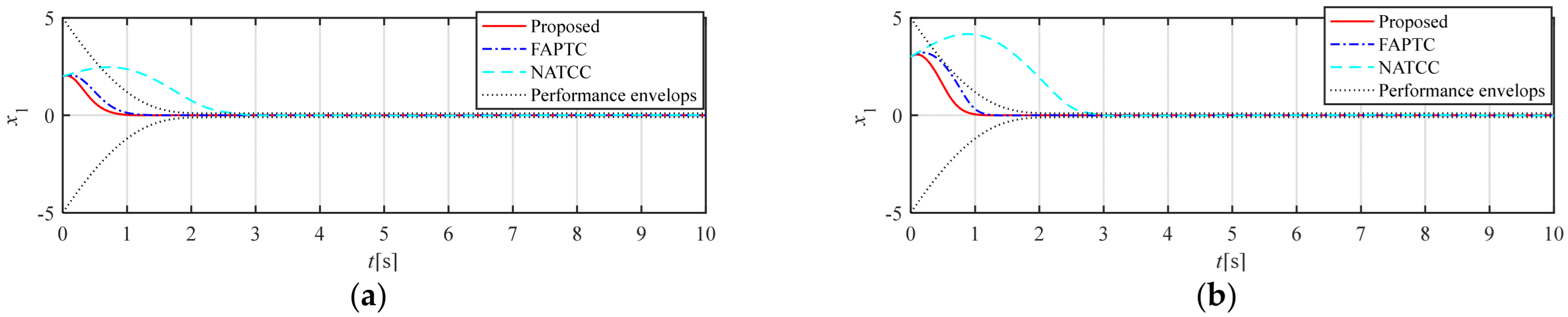
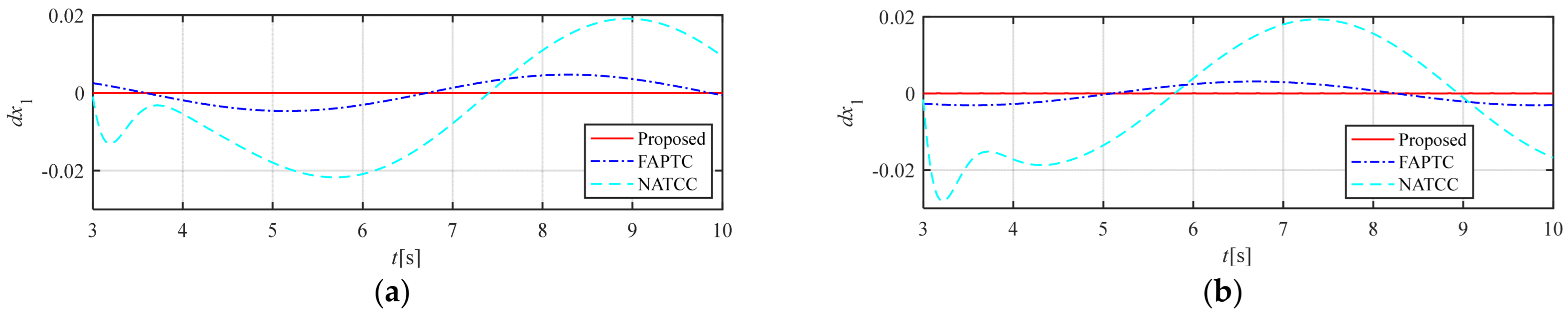
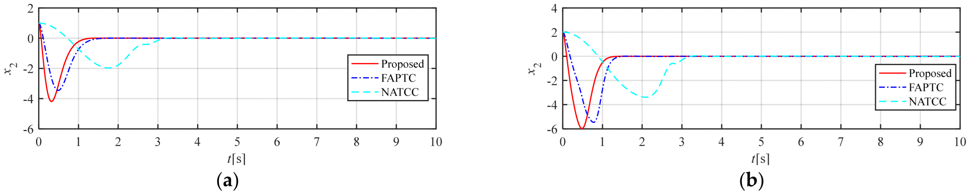
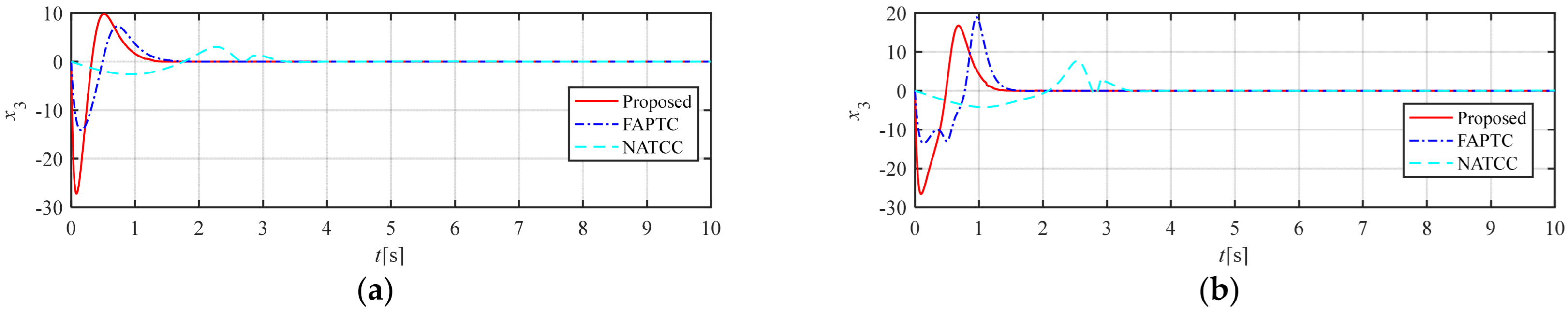
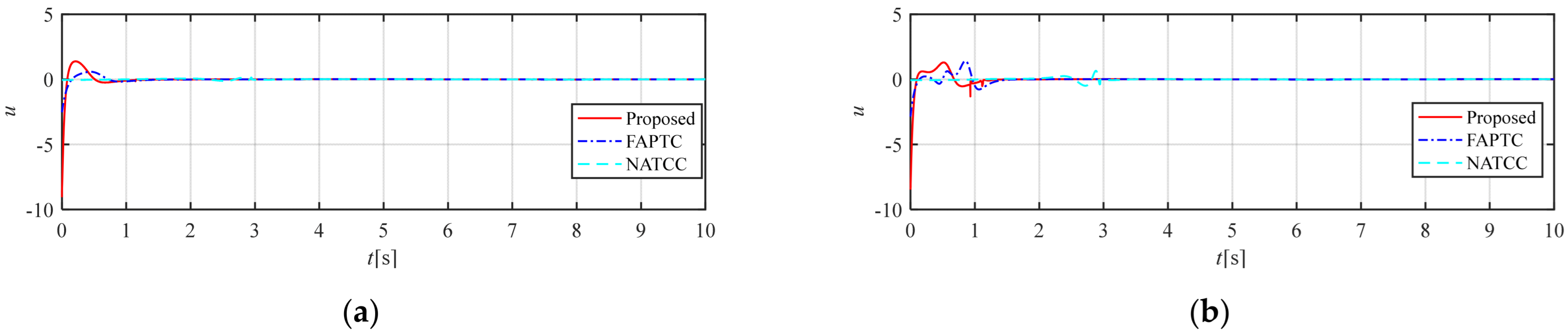
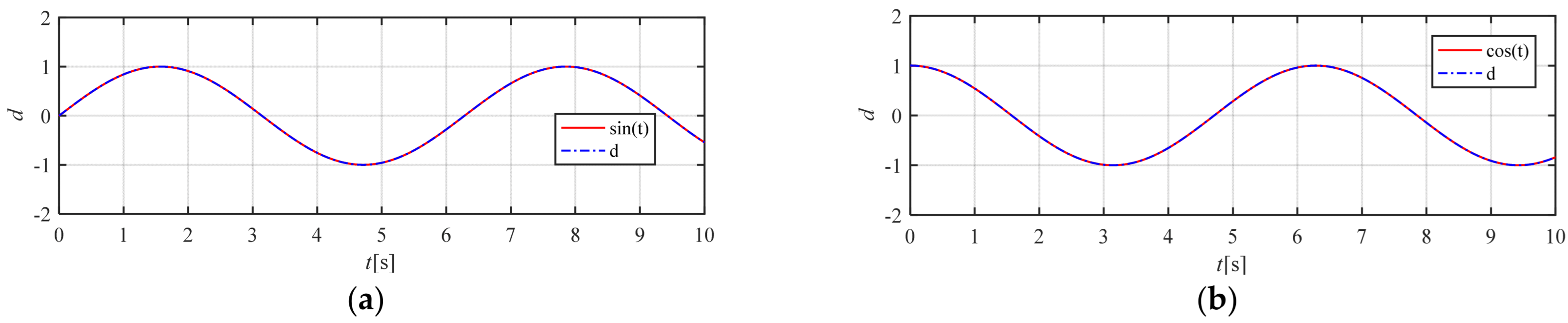
4.1. Simulation of the Proposed Control Scheme on the Third-Order Integral Chain System

Introduce a third-order integral chain system, ${\dot{x}}_1=x_2$, ${\dot{x}}_2=x_3$, ${\dot{x}}_3=100u+d$, where $d$ is the total disturbance momentum. The desired value of the state is $x_{1c}=x_{2c}=x_{3c}=0$. Compare the performance of the method proposed in this paper with the alternative predefined time tracking controller based on a novel C∞ performance function (FAPTC) in Reference [28] and the a new arbitrary time convergence controller (NATCC) in Reference [35]. The control method parameters in this paper are shown in

Table 1. The control method parameters in Section 4.1.

Parameter	Value	Parameter	Value
${\alpha }_1$	0.2	${\mu }_1$	1
$p_1$	2	$q_1$	1
$T_1$	1	$\beta$	1
$\rho \left(0\right)$	5	$\rho \left(T\right)$	0.1
$T$	3	$\alpha$	0.38
$\mu$	1	$p$	1
$q$	1

.

The following are the simulation results with initial values of $x_1=2$, $x_2=1$, $x_3=0$, $d=\sin t$ and $x_1=3$, $x_2=2$, $x_3=0$, $d=\cos t$.

The state variables $x_1$, $x_2$, $x_3$ and $u$ are provided in Figure 2, Figure 3, Figure 4, Figure 5 and Figure 6. The third-order state variables all converge to the preset range within the predefined time. As shown in Figure 2, our method and FAPTC can always be controlled within the performance envelope, but NATCC does not possess such properties, and the performance envelope has the properties described in Remarks 3 and 4. Moreover, from Figure 3. Time histories of state variables $d{x}_1$: (a) $x_1=2$, $x_2=1$, $x_3=0$, $d=\sin t$; (b) $x_1=3$, $x_2=2$, $x_3=0$, $d=\cos t$, it can be seen that our method can accurately converge to 0, verifying the statements in Remarks 5 and 6 of the proposed control method. As shown in Figure 7. Time histories of state variables $d$: (a) $x_1=2$, $x_2=1$, $x_3=0$, $d=\sin t$; (b) $x_1=3$, $x_2=2$, $x_3=0$, $d=\cos t$, the predefined-time nonsingular sliding mode observer proposed in this article can accurately observe time-varying disturbances, verifying the correctness of the properties described in Remark 2.

As can be seen from Figure 2, both the method proposed in this paper and FAPTC can converge along the preset performance envelope within the predefined time, and the convergence speed of the proposed method is better. Although NATCC can also converge within the predefined time, its convergence speed is slow and it cannot be constrained within the corresponding envelope. Figure 3 shows the convergence of the three methods after the preset time. All three methods can converge to near zero after the predefined time, but the proposed method can completely converge to zero, with better stability and convergence than FAPTC and NATCC. Figure 4 and Figure 5 show the derivative information of the state variable $x_1$, whose convergence is consistent with that of the state variable $x_1$. Figure 6 is the control quantity curve. The control quantities of the proposed method and FAPTC are similar in magnitude, while the initial control quantity of NATCC is small, but there is jitter near the preset time of 3 s, which is determined by the convergence function of this method and has relatively poor stability. Figure 7 is the simulation result of the observer proposed in this paper, from which it can be seen that the observer can well observe the error information.

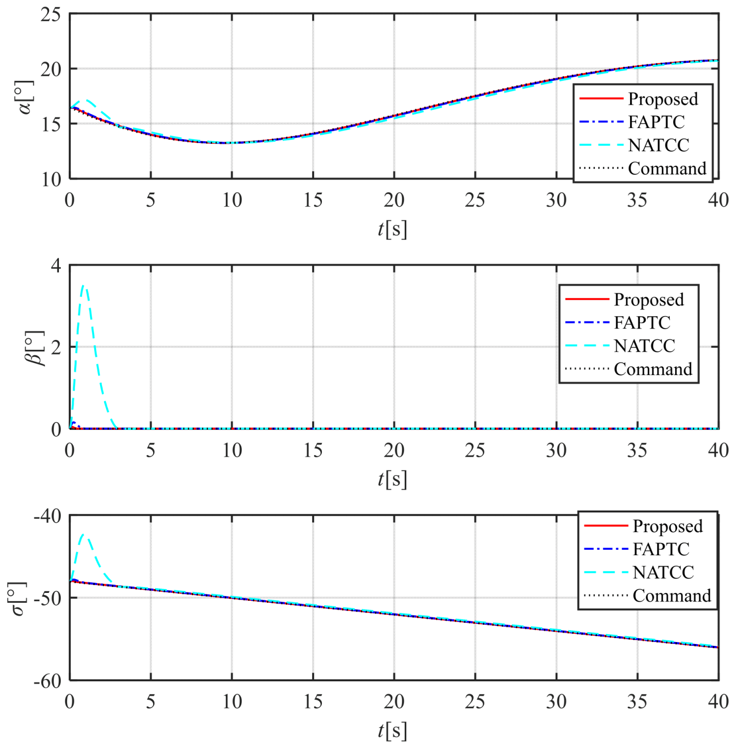
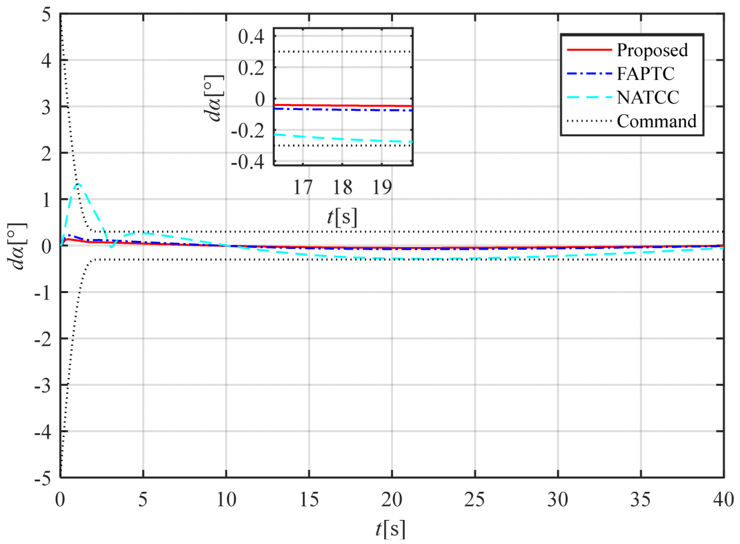
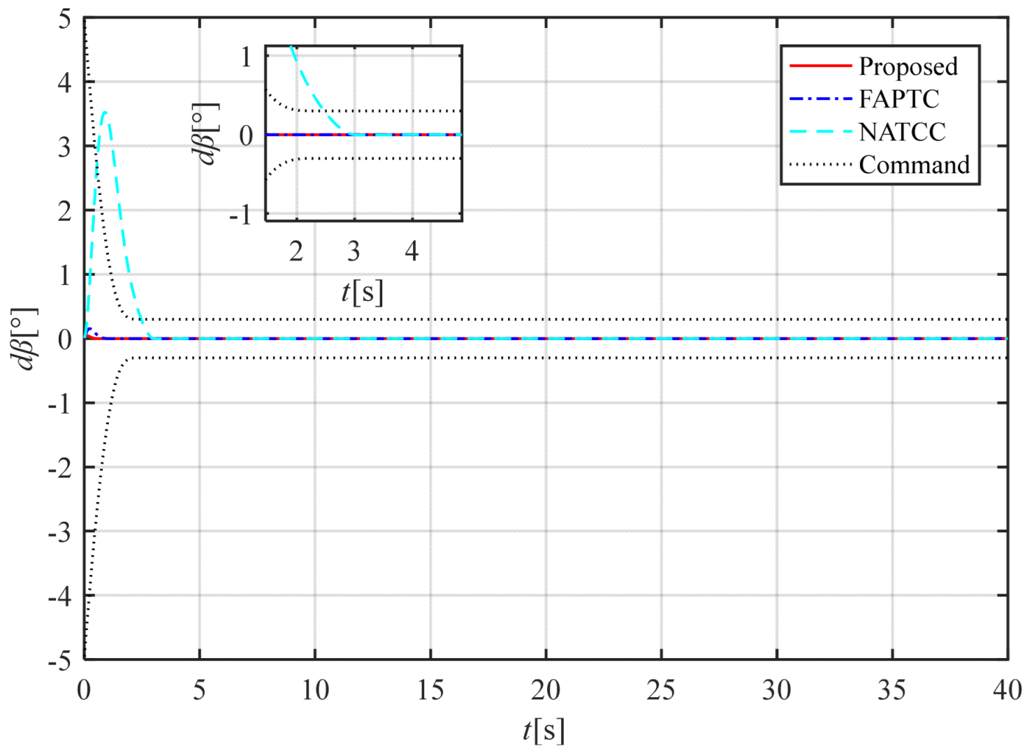
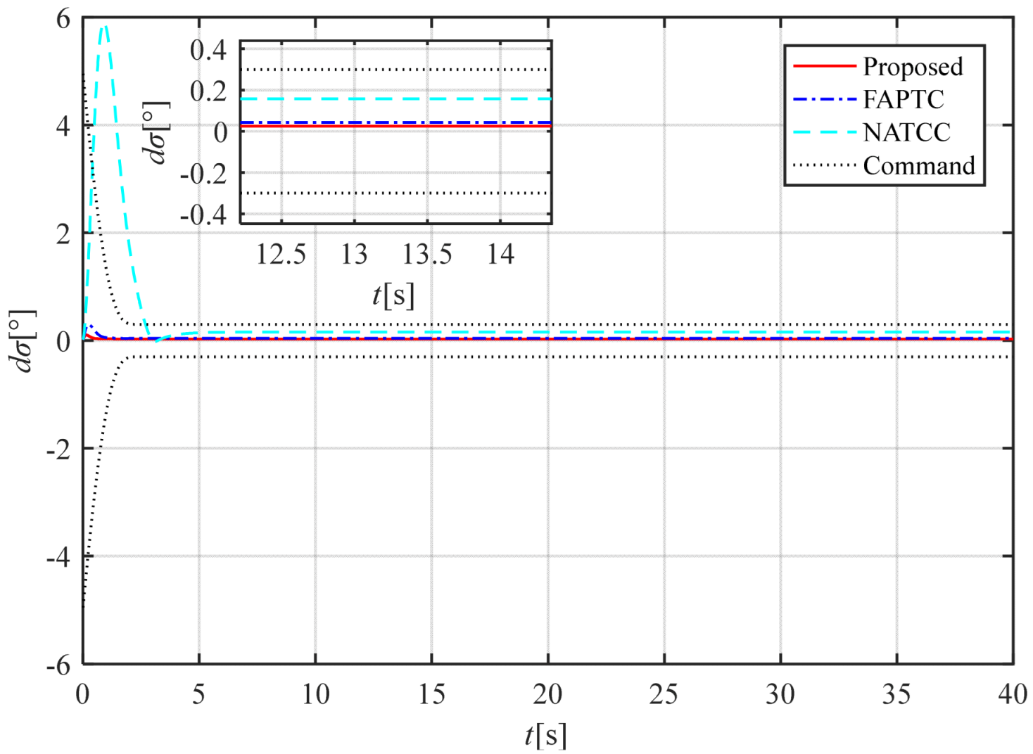
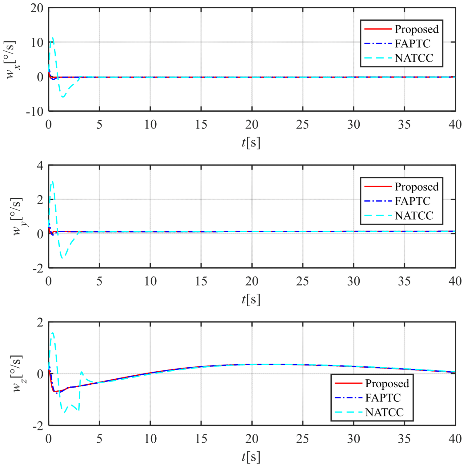
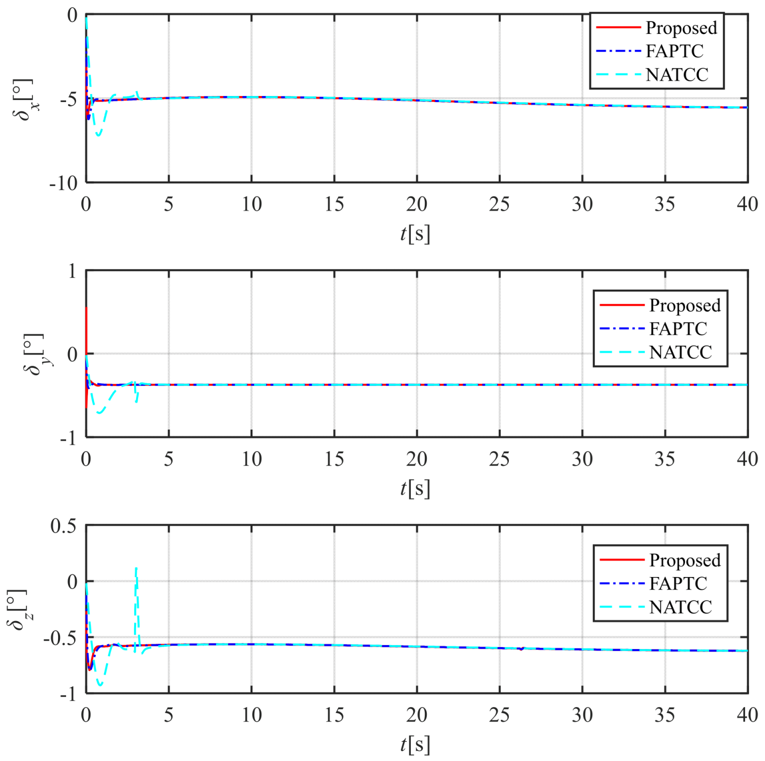
4.2. Simulation of the Proposed Control Scheme on the Aerospace Aircraft

The structural and aerodynamic parameters of the aerospace aircraft are shown in

Table 2. Parameters of the aerospace aircraft.

Parameter	Value	Parameter	Value
$m/\mathrm{kg}$	5000.0	$Sm/{\mathrm{m}}^2$	2.0
$L/\mathrm{m}$	6.0	$I_{xx}/\mathrm{kg}\cdot {\mathrm{m}}^2$	10,000.0
$I_{xy}/\mathrm{kg}\cdot {\mathrm{m}}^2$	3000.0	$I_{yy}/\mathrm{kg}\cdot {\mathrm{m}}^2$	13,000.0
$I_{zz}/\mathrm{kg}\cdot {\mathrm{m}}^2$	8000.0	$C_{Mx}^{\alpha }$	0.0033
$C_{My}^{\beta }$	0.036	$C_{Mz}^{\alpha }$	0.045
$C_{Mx}^0$	0.004	$C_{My}^0$	0.0032
$C_{Mz}^0$	0.036	$C_{Mx}^{{\delta }_x}$	0.4
$C_{My}^{{\delta }_y}$	0.41	$C_{Mz}^{{\delta }_z}$	0.45

.

The control method parameters in this paper are shown in

Table 3. The control method parameters in Section 4.2.

Parameter	Value	Parameter	Value
${\alpha }_1$	0.2	${\mu }_1$	1
$p_1$	2	$q_1$	1
$T_1$	1	$\beta$	1
$\rho \left(0\right)$	$5°$	$\rho \left(T\right)$	$0.3°$
$T$	3	$\alpha$	0.2
$\mu$	1	$p$	1
$q$	1

The initial angle is $\alpha =16.42°$, $\beta =0°$, $\sigma =-48.06°$.

.

The comparative simulation results of the three methods are as follows:

The three-channel attitude angle tracking curve is shown in Figure 8, and the three-channel attitude angle deviation curve is shown in Figure 9, Figure 10 and Figure 11. The method proposed in this paper and FAPTC can always be controlled within the performance envelope, but NATCC does not possess such properties, and the performance envelope has the properties described in Remarks 3 and 4. From Figure 9, Figure 10 and Figure 11, it can be seen that the attitude angle deviation of our proposed method is significantly smaller than that of the FAPTC method, and it has the properties described in Remarks 5 and 6. From the angular rates curve and rudder deviation angle curve, it can be seen that the maximum angular velocity and rudder deviation angle of our proposed method are both smaller than NATCC. Therefore, considering the control deviation and control quantity, the method proposed in this paper is superior to FAPTC and NATCC.

As shown in Figure 8, the attitude angle error of NATCC is significantly larger than that of the method proposed in this paper. By examining the attitude angle errors in Figure 9, Figure 10 and Figure 11, it can be observed that NATCC exhibits larger attitude angle errors. The proposed method achieves zero attitude angle error after the preset time, whereas the attitude angle error of FAPTC fails to fully converge to zero. According to the angular velocity curve in Figure 12, due to the larger attitude angle error of NATCC, both the variation range and rate of its angular velocity curve are greater. In contrast, the proposed method features smaller angular velocity and a stable variation rate. From the rudder deflection angle curve in Figure 13, it can be seen that the control magnitude of the proposed method is similar to that of FAPTC. However, NATCC shows a larger variation range and higher variation rate in control magnitude. Figure 14 presents the observation error curve of the observer. As indicated by the curve characteristics, the observer demonstrates excellent convergence performance, with errors decaying rapidly over time and stabilizing within the preset range, which fully verifies the effectiveness and reliability of the observation algorithm.

Based on the comprehensive analysis of the above simulation results, the method proposed in this paper not only ensures that the initial tracking error converges within the predefined time, but also guarantees that any error generated within the error boundary during the subsequent control process can converge within the predefined time. Compared with the two comparative methods, this method demonstrates superior performance in terms of global convergence and anti-interference capability.

5. Conclusions

To address the attitude control problem of aerospace vehicles with model parameter uncertainties and external disturbances, this study proposes a novel predefined-time control approach incorporating a predefined-time disturbance observer to enhance global convergence performance and disturbance rejection capability. First, an adaptive predefined-time nonsingular sliding-mode disturbance observer is designed to estimate modeling uncertainties and external disturbances, ensuring fast convergence while mitigating chattering. Then, by integrating a new performance function with nonsingular predefined-time sliding-mode control, a novel global predefined-time controller suitable for arbitrary-order systems is developed. Simulation results demonstrate that compared with existing predefined-time controllers, the proposed controller guarantees that attitude tracking errors converge to zero not only within a preset time interval but also globally (i.e., over the entire time domain). Notably, this research does not address global predefined-time control under actuator failures and saturation conditions, which will be explored in future research.

References

1. Mueller, G.E.; Lepore, D.F. The K-1 reusable aerospace vehicle: Managing to achieve low cost. Acta Astronaut. 2000, 46, 199–202. [Google Scholar] [CrossRef]
2. McHenry, R.L.; Long, A.D.; Cockrell, B.F.; Thibodeau, J.R., III; Brand, T.J. Space shuttle ascent guidance navigation and control. J. Astronaut. Sci. 1979, 27, 1–38. [Google Scholar]
3. Paez, C. The development of the X-37 re-entry vehicle. In Proceedings of the 40th AIAA/ASME/SAE/ASEE Joint Propulsion Conference and Exhibit, Fort Lauderdale, FL, USA, 11–14 July 2004; p. 4186. [Google Scholar]
4. Chu, L.; Li, Q.; Gu, F.; Du, X.; He, Y.; Deng, Y. Design, modeling, and control of morphing aircraft: A review. Chin. J. Aeronaut. 2021, 35, 220–246. [Google Scholar] [CrossRef]
5. Zhao, K.; Song, J.; Ai, S.; Xu, X.; Liu, Y. Active Fault-Tolerant Control for Near-Space Hypersonic Vehicles. Aerospace 2022, 9, 237. [Google Scholar] [CrossRef]
6. Wang, X.; Xu, B. Robust Adaptive Control of Hypersonic Flight Vehicle With Aero-Servo-Elastic Effect. IEEE Trans. Aerosp. Electron. Syst. 2023, 59, 1955–1964. [Google Scholar] [CrossRef]
7. Qian, C.; Lin, W. Recursive Observer Design, Homogeneous Approximation, and Nonsmooth Output Feedback Stabilization of Nonlinear Systems. IEEE Trans. Autom. Control. 2006, 51, 1457–1471. [Google Scholar] [CrossRef]
8. Kayacan, E. Sliding mode control for systems with mismatched time-varying uncertainties via a self-learning disturbance observer. Trans. Inst. Meas. Control. 2018, 41, 2039–2052. [Google Scholar] [CrossRef]
9. Li, G.; Chen, X.; Yu, J.; Liu, J. Adaptive Neural Network-Based Finite-Time Impedance Control of Constrained Robotic Manipulators With Disturbance Observer. IEEE Trans. Circuits Syst. II: Express Briefs 2022, 69, 1412–1416. [Google Scholar] [CrossRef]
10. Hu, Q.; Jiang, B. Continuous Finite-Time Attitude Control for Rigid Spacecraft Based on Angular Velocity Observer. IEEE Trans. Aerosp. Electron. Syst. 2018, 54, 1082–1092. [Google Scholar] [CrossRef]
11. Park, J.; Bang, H.; Park, K.; Lee, S. Cascade nonlinear observer design for large amplitude of slosh variables in spacecraft maneuver with liquid propellant tank. Acta Astronaut. 2023, 213, 35–48. [Google Scholar] [CrossRef]
12. Bai, Y.; Wang, X.; Xu, J.; Cui, N. Adaptive quaternion tracking with nonlinear extended state observer. Acta Astronaut. 2017, 139, 494–501. [Google Scholar] [CrossRef]
13. Song, Y.; Chen, X.; Yin, Z.; Liao, Y.; Wei, C. Robust attitude coordinated control for gravi-tational-wave detection spacecraft formation with large-scale communication delays. Acta Astronaut. 2024, 221, 34–45. [Google Scholar] [CrossRef]
14. Zhang, Y.; Ma, M.; Yang, X.; Song, S. Dis-turbance-observer-based fixed-time control for 6-DOF spacecraft rendezvous and docking operations under full-state constraints. Acta Astronaut. 2023, 205, 225–238. [Google Scholar] [CrossRef]
15. Chen, J.; Chen, Z.; Zhang, H.; Xiao, B.; Cao, L. Predefined-Time Observer-Based Nonsingular Sliding-Mode Control for Spacecraft Attitude Stabili-zation. IEEE Trans. Circuits Syst. II Express Briefs 2024, 71, 1291–1295. [Google Scholar]
16. Xie, S.; Chen, Q. Predefined-Time Disturb-ance Estimation and Attitude Control for Rigid Space-craft. IEEE Trans. Circuits Syst. II Express Briefs 2024, 71, 2089–2093. [Google Scholar]
17. Eliker, K.; Zhang, W.D. Finite-time adaptive integral backstepping fast terminal sliding mode control application on quadrotor UAV. Int. J. Control. Autom. Syst. 2020, 18, 415–430. [Google Scholar] [CrossRef]
18. Wang, J.; Zong, Q.; Su, R.; Tian, B.L. Continuous high order sliding mode controller design for a flexible air-breathing hypersonic vehicle. ISA Trans. 2014, 53, 690–698. [Google Scholar] [CrossRef]
19. Zhang, L.; Wei, C.Z.; Wu, R.; Cui, N.G. Fixed-time extended state observer based non-singular fast terminal sliding mode control for a VTVL reusable launch vehicle. Aerosp. Sci. Technol. 2018, 82, 70–79. [Google Scholar] [CrossRef]
20. You, M.; Zong, Q.; Tian, B.L.; Zhao, X.Y.; Zeng, F.L. Comprehensive design of uniform robust exact disturbance observer and fixed-time controller for reusable launch vehicles. Iet Control. Theory Appl. 2018, 12, 638–648. [Google Scholar] [CrossRef]
21. Sánchez-Torres, J.D.; Sanchez, E.N.; Loukianov, A.G. Predefined-time stability of dynamical systems with sliding modes. In Proceedings of the American Control Conference (ACC), Chicago, IL, USA, 1–3 July 2015; pp. 5842–5846. [Google Scholar]
22. Ju, X.Z.; Wei, C.Z.; Xu, H.C.; Wang, F. Fractional-order sliding mode control with a predefined-time observer for VTVL reusable launch vehicles under actuator faults and saturation constraints. ISA Trans. 2022, 129, 55–72. [Google Scholar] [CrossRef]
23. Su, Y.; Shen, S. Adaptive predefined-time fault-tolerant attitude tracking control for rigid space-craft with guaranteed performance. Acta Astronaut. 2023, 214, 677–688. [Google Scholar] [CrossRef]
24. Becerra, H.M.; Vázquez, C.R.; Arechavaleta, G.; Delfin, J. Predefined-Time Convergence Control for High-Order Integrator Systems Using Time Base Generators. IEEE Trans. Control. Syst. Technol. 2018, 26, 1866–1873. [Google Scholar] [CrossRef]
25. Guo, C.; Hu, J. Time Base Generator-Based Practical Predefined-Time Stabilization of High-Order Systems With Unknown Disturbance. IEEE Transac-Tions Circuits Syst. II Express Briefs. 2023, 70, 2670–2674. [Google Scholar] [CrossRef]
26. Ning, B.; Han, Q.; Zuo, Z. Bipartite Consen-sus Tracking for Second-Order Multiagent Systems: A Time-Varying Function-Based Preset-Time Approach. IEEE Trans. Autom. Control. 2020, 66, 2739–2745. [Google Scholar] [CrossRef]
27. Liu, Y.; Liu, X.; Jing, Y.; Zhang, Z. A Novel Finite-Time Adaptive Fuzzy Tracking Control Scheme for Nonstrict Feedback Systems. IEEE Trans. Fuzzy Syst. 2019, 27, 646–658. [Google Scholar] [CrossRef]
28. Li, J.; Du, J. Predefined-time tracking control of a class of nonlinear systems via a novel C∞ performance function. Int. J. Robust. Nonlinear Control. 2024, 34, 3586–3601. [Google Scholar] [CrossRef]
29. Sánchez-Torres, J.D.; Sánchez-Torres, J.D.; Gómez–Gutiérrez, D.; López, E.; Loukianov, A.G. A class of predefined-time stable dynamical systems. Ima J. Math. Control. Inf. 2018, 35, 1–29. [Google Scholar] [CrossRef]
30. Jia, C.; Liu, X.; Xu, J. Predefined-Time Nonsingular Sliding Mode Control and Its Application to Nonlinear Systems. IEEE Trans. Ind. Inform. 2024, 20, 5829–5837. [Google Scholar] [CrossRef]
31. Zhang, M.; Zang, H.; Bai, L. A New Predefined-Time Sliding Mode Control Scheme for Synchronizing Chaotic Systems. SSRN Electron. J. 2022, 164, 112745. [Google Scholar]
32. Zuo, Z.; Tie, L. Distributed robust finite-time nonlinear consensus protocols for multi-agent systems. Int. J. Syst. Sci. 2014, 47, 1366–1375. [Google Scholar] [CrossRef]
33. Liu, Y.; Liu, X.; Jing, Y. Adaptive neural networks finite-time tracking control for non-strict feedback systems via prescribed performance. Inf. Sci. 2018, 468, 29–46. [Google Scholar] [CrossRef]
34. Wei, C.; Gui, M.; Zhang, C.; Liao, Y.; Dai, M.; Luo, B. Adaptive Appointed-Time Consensus Control of Networked Euler–Lagrange Systems With Connectivity Preservation. IEEE Trans. Cybern. 2021, 52, 12379–12392. [Google Scholar] [CrossRef] [PubMed]
35. Pal, A.K.; Kamal, S.; Nagar, S.K.; Bandyopadhyay, B.; Fridman, L.M. Design of controllers with arbitrary convergence time. Automatica 2020, 112, 108710. [Google Scholar] [CrossRef]
Figure 1. Adaptive global predefined-time control method.
Aerospace 12 00580 g001
Figure 2. Time histories of state variables x 1 : (a) x 1 = 2 , x 2 = 1 , x 3 = 0 , d = sin t ; (b) x 1 = 3 , x 2 = 2 , x 3 = 0 , d = cos t .
Aerospace 12 00580 g002
Figure 3. Time histories of state variables d x 1 : (a) x 1 = 2 , x 2 = 1 , x 3 = 0 , d = sin t ; (b) x 1 = 3 , x 2 = 2 , x 3 = 0 , d = cos t .
Aerospace 12 00580 g003
Figure 4. Time histories of state variables x 2 : (a) x 1 = 2 , x 2 = 1 , x 3 = 0 , d = sin t ; (b) x 1 = 3 , x 2 = 2 , x 3 = 0 , d = cos t .
Aerospace 12 00580 g004
Figure 5. Time histories of state variables x 3 : (a) x 1 = 2 , x 2 = 1 , x 3 = 0 , d = sin t ; (b) x 1 = 3 , x 2 = 2 , x 3 = 0 , d = cos t .
Aerospace 12 00580 g005
Figure 6. Time histories of state variables u : (a) x 1 = 2 , x 2 = 1 , x 3 = 0 , d = sin t ; (b) x 1 = 3 , x 2 = 2 , x 3 = 0 , d = cos t .
Aerospace 12 00580 g006
Figure 7. Time histories of state variables d : (a) x 1 = 2 , x 2 = 1 , x 3 = 0 , d = sin t ; (b) x 1 = 3 , x 2 = 2 , x 3 = 0 , d = cos t .
Aerospace 12 00580 g007
Figure 8. Time histories of the attitude angles α , β , and σ .
Aerospace 12 00580 g008
Figure 9. Time histories of the tracking error α .
Aerospace 12 00580 g009
Figure 10. Time histories of the tracking error β .
Aerospace 12 00580 g010
Figure 11. Time histories of the tracking error σ .
Aerospace 12 00580 g011
Figure 12. Time histories of the angular rates w x , w y , and w z .
Aerospace 12 00580 g012
Figure 13. Time history of rudder deviation angle δ x , δ y , and δ z .
Aerospace 12 00580 g013
Figure 14. Time history of observed value deviation d ˜ x , d ˜ y , and d ˜ z .
Aerospace 12 00580 g014