Dynamic Modeling and Safety Analysis of Whole Three-Winch Traction System of Shipboard Aircraft

Abstract

The winch traction system for shipboard aircraft, when operating in a marine environment, is subjected to additional forces and moments due to the complex motion of the hull. These loads pose significant threats to the safety of the aircraft during the traction process. To address the safety issues under complex sea conditions, this paper adopts harmonic functions to describe the rolling, pitching, and heaving motions of the hull. A theoretical analytical model of the three-winch traction system, considering the intricate coupling motions of the ship, is established. Unlike previous studies that often simplify ship motion or focus on single-component modeling, this work develops a complete, whole-system dynamic model integrating the winch system, rope, aircraft structure, and ship interaction. The dynamic characteristics of the small-deck winch traction system are investigated, with particular focus on the influence of the rear winch position, driving trajectory, and ship motion on the system’s dynamics and safety. This research is innovative in systematically exploring the dynamic safety behavior of a three-winch traction system operating under small-deck conditions and complex sea states. The results show that as the distance between the two rear winches increases, the lateral force on the tire decreases. Additionally, as the aircraft’s turning angle increases, the front winch rope force also increases. Moreover, with higher sea condition levels and wind scales, the maximum lateral force on the tires increases, leading to a significant reduction in the stability and safety of the winch traction system. This is particularly critical when the sea condition level exceeds 3 and the wind scale exceeds 6, as it increases the risk of tire sideslip or off-ground events. This research has substantial value for enhancing the safety and stability of winch traction systems on small decks, and also provides a theoretical basis for traction path design, winch position optimization, and the extension of the service life of key system components, demonstrating strong engineering applicability.

1. Introduction

Under complex sea conditions, the traction safety of shipboard aircraft faces significant challenges [1]. At present, shipboard aircraft traction primarily relies on two methods, tractor traction and winch traction, as illustrated in Figure 1. Tractor traction involves the use of a dedicated towing vehicle connected to the aircraft’s nose landing gear or fuselage towing point. The vehicle provides motive power to move the aircraft. This method offers high flexibility and is well-suited for multi-path operations, and is widely used in airport taxiing and ground handling.

However, in space-constrained environments such as ship decks, the maneuverability of the towing vehicle is significantly limited, and the operation places high demands on personnel skills. In contrast, winch traction employs a fixed winch system installed on the ship, which connects to the aircraft via steel cables or high-strength ropes. By controlling the retraction and release of the cable, the aircraft can be maneuvered as required. Compared to tractor traction, winch traction is better suited to confined spaces with predefined routes. It offers advantages such as a simpler structure, lower cost, and higher control precision.

Investigators have carried out considerable research on the modeling and stability of the traction system and have made notable progress. Zhao et al. [3] utilized a tire model represented by springs and dampers to analyze the stability of tractors and airplanes during traction processes. They conducted simulations of typical traction conditions, and the simulation results provide guidance for the driving stability of tractors and airplanes. Wang et al. [4] used a multibody dynamic model composed of a tractor, a traction rod, and an aircraft to discuss and analyze the folding trend of the aircraft traction system during the braking process. In the case of turning braking, the relationship between the maximum braking torque and the relative turning angle is obtained. Jiang et al. [5] established a multibody dynamics model (MBD) of the aircraft and studied the influence of the torsional damping of the front landing gear on the directional stability of the aircraft. Linn et al. [6] derived a four-degrees-of-freedom mathematical model for predicting and analyzing the behavior of carrier-based aircraft under external control forces. Huang et al. [7] developed a six-degrees-of-freedom aircraft dynamics model comprising the fuselage, the landing struts, the nose wheel, and the main wheels to conduct a series of dynamic analyses. The results indicate that pre-rotating the aircraft wheels is an effective method for reducing the drag load exerted on the wheels during landing. He et al. [8] proposed a modeling method to integrate a coordinate transformation model, a ship velocity transformation model, and a landing gear torque model into a six-degrees-of-freedom helicopter model. The approach effectively captures the motion characteristics of real helicopters. Thota et al. [9] investigated the relationship between nose landing gear vibration and tire force changes in passenger aircraft. Daniels et al. [10] proposed a method for establishing a nonlinear model of the main gear of the A-6 Intruder and verified it with the static and dynamic test data. Zhou et al. [11] developed a six-degrees-of-freedom (DOF) dynamic platform virtual testbed and created a virtual prototype model of a nonlinear carrier-based aircraft traction system by ADAMS and MATLAB/Simulink. Simulation results indicate that the stability of the traction system can be significantly improved. Qi et al. [12] established a four-degrees-of-freedom time-varying nonlinear dynamic model for a carrier-based aircraft without a towed trailer system, and analyzed the lateral stability of the traction system. Yoo et al. [13] proposed a dynamic simulation model for aircraft that considers six degrees of freedom of platform motion to analyze the motion characteristics of aircraft on the deck. Liu et al. [14] transformed the rodless traction-based carrier aircraft system into a tractor–trailer system to research trajectory planning and tracking for improving the efficiency and safety of the system.

In addition to the aforementioned studies, many researchers have also conducted related work on the trajectory tracking and control of shipboard aircraft. Wang et al. [2] designed a path-following controller, and used compensated tracking technology for the direction control, and verified the path-following performance under closed-loop conditions through interactive co-simulation tests. Yu et al. [15] used the RRT * (Rapidly exploring Random Tree Star) algorithm to generate trajectories for the tractor-aircraft system and developed a double-layer closed-loop controller for trajectory tracking of the tractor system on deck; the controller is designed to handle operations under incomplete constraints. Wang et al. [16] proposed an efficient hierarchical initialization technique based on the Dubins curve method and designed a model predictive controller for tracking the resulting reference trajectory. Su et al. [17] addressed the limitations of existing fully automated methods in handling complex environments. They proposed a path planning approach for carrier-based aircraft on the deck that combines human expertise with intelligent search techniques. The feasibility and effectiveness of this method were validated through simulations. Marantos et al. [18] reported a robust control scheme to solve the trajectory tracking problem of small unmanned helicopters under model uncertainty and external interference through the cascading operation of position and attitude control modules. Raptis et al. [19] presented a model-based tracking control design method for mini-unmanned helicopters; the nominal linear state-space model controller successfully captures the coupled multivariable dynamics of small helicopters. Wu et al. [20] studied the taxiing path planning in the actual deck environment, and the model predictive control (MPC) theory and dynamic multi-step optimization algorithm were used to search for the path. Based on a variable structure control strategy, Wang et al. [21] proposed a dynamic sliding trajectory tracking automatic steering controller for the tractor; the research results show that the controller can effectively suppress the impact of uncertain parameters on the tracking performance of the tractor. By applying the model predictive control theory to path searching, Wu et al. [20] developed a dynamic weight heuristic function and presented a dynamic multi-step optimization algorithm. Yu et al. [22] established a multi-precision UAV path planning system using MATLAB for safety inspections in hazardous areas. Woo et al. [23] researched implementable integrated technology for path planning, trajectory generation, and trajectory tracking control for the autonomy of aircraft missions. Wang et al. [24] investigated the path planning techniques and the algorithms for carrier-based aircraft under three different scheduling modes.

Although there is abundant literature on traction modeling and trajectory control, most studies focus on tractor traction technology. Considering the limited space on small decks for shipboard aircraft, it is difficult for tractor traction to meet the operational requirements of such environments. Winch traction, with its high stability and safety, deserves more attention and in-depth research. Moreover, there is currently a lack of comprehensive system-level modeling and dynamic characteristic analysis of winch traction systems under complex sea conditions.

For this, this paper establishes a comprehensive system-level dynamic model of the whole system of the shipboard aircraft three-winch traction system, encompassing the coupled interactions between the winch, rope, aircraft, and ship. The model comprehensively considers ship motions, including rolling, pitching, and heaving, with a focus on analyzing the dynamic response characteristics of the winch traction system in small-deck environments. This study systematically investigates the effects of rear winch positions, towing trajectories, and ship motions on the system’s dynamics and safety, revealing response features and potential risks under complex sea conditions. The results provide important guidance for improving the safety and stability of three-winch traction systems and offer theoretical support for the application and development of winch traction technology on small ship decks.

2. Modeling of the Traction Dynamics of the Shipboard Aircraft with Three Winches

Dynamic modeling of the shipboard aircraft traction system is fundamental to the system’s safety analysis. The accuracy of this analysis depends on the completeness and appropriateness of the model. Given the uncertainties of ship motion under complex sea conditions, constructing a dynamic model that fully aligns with real-world scenarios is challenging. To address this, the ship’s motion model is simplified, and a dynamic model encompassing the winch, ropes, landing gear, tires, and ship motion is developed in this research.

2.1. Modeling of Three-Winch Traction Dynamics of Shipboard Aircraft

Based on the working principle of winch traction for shipboard aircraft, a dynamic model of the winch traction system is established. The schematic diagram of the winch traction system is illustrated in Figure 1a. In this setup, the front winch is connected to the traction point of landing gear 1 (Tire 1) via a rope, rear winch 1 is connected to the traction point of landing gear 2 (Tire 2), and rear winch 2 is connected to the traction point of landing gear 3 (Tire 3). During warehousing traction, the front winch provides the primary traction force, while the rear winches offer sufficient back traction force to stabilize the aircraft and prevent it from moving back and forth. When pulling the aircraft out of the warehouse, the two rear winches provide the main traction, with the front winch supplying the necessary back traction.

2.1.1. Fuselage Model

The fuselage is simplified as a rigid body to calculate the external forces and moments acting on the traction system. The classical Newton–Euler equation is applied to establish the equation of motion for the system. The centroid acceleration of the shipboard aircraft is ${\ddot{X}}_{pi}$, and one can obtain

$${\ddot{X}}_{pi}={\displaystyle \frac{1}{m}}\left[\Sigma F_{xi};\Sigma F_{yi};\Sigma F_{zi}\right]$$

(1)

where m is the mass of the aircraft; F = $\left[\Sigma F_{xi};\Sigma F_{yi};\Sigma F_{zi}\right]$ is the resultant external force acting on the aircraft system.

The Euler dynamic equation is written as

$$\begin{array}{l}{\dot{\omega }}_x=\left(M_{px}+\left(I_{py}-I_{pz}\right)\ast {\omega }_y{\omega }_z\right)/I_{px}\\ {\dot{\omega }}_y=\left(M_{py}+\left(I_{pz}-I_{px}\right)\ast {\omega }_x{\omega }_z\right)/I_{py}\\ {\dot{\omega }}_x=\left(M_{pz}+\left(I_{px}-I_{py}\right)\ast {\omega }_x{\omega }_y\right)/I_{pz}\end{array}$$

(2)

where M_px, M_py, and M_pz are moments around the x-, y-, and z-directions, respectively; ω_x, ω_y, and ω_z are the angular velocities of the aircraft around the x-, y-, and z-axes, respectively, and $I=\left[I_{px};I_{py};I_{px}\right]$ is the moment of inertia matrix.

2.1.2. The Winch Model

The winch system provides traction to pull the aircraft via a rope. Accordingly, the capstan and rope are modeled separately in this section.

(1)

The capstan

The force analysis of the rope on the traction drum is illustrated in Figure 2. The rope is wound around the traction capstan, and a differential segment of the arc on the capstan, dα, is selected for the force analysis. As the winch rotates clockwise, the traction force on the rope is F + dF. Due to friction, the force is reduced by dF through the differential arc dα, resulting in an output force of F. The dF is the front pressure of the rope to the capstan; μ is the friction coefficient between the rope and the capstan groove, and μ = 0.5.

According to Figure 2, the following equation can be obtained:

$$\begin{array}{l}\left(F+dF\right)\cos {\displaystyle \frac{d\alpha }{2}}=\mu dN+F\cos {\displaystyle \frac{d\alpha }{2}}\\ \left(F+dF\right)\sin {\displaystyle \frac{d\alpha }{2}}+F\sin {\displaystyle \frac{d\alpha }{2}}=dN\end{array}$$

(3)

Since the differential element dα is very small, there exists $\sin {\displaystyle \frac{d\alpha }{2}}\approx {\displaystyle \frac{d\alpha }{2}}$ and $\cos {\displaystyle \frac{d\alpha }{2}}\approx 1$, and because of $dF<F$ the following equations can be obtained:

$$\begin{array}{l}\mathrm{dF}=\mu dN\\ Fd\alpha =dN\end{array}$$

(4)

And then one can get

$${\displaystyle \frac{dF}{F}}=\mu d\alpha$$

(5)

Integrating Equation (5) leads to

$$F_1=F_2{e}^{\mu \alpha }$$

(6)

where α is the sliding angle; F₁ is the pulling force of the tight end; F₂ is the pulling force of the loose end.

(2)

Rope model

The rope, being a typical flexible object, is simplified in this research to be an ideal spring model. As shown in Figure 3, Point 1 is connected to the winch, while Point 2 is attached to the aircraft’s traction point.

The calculation formula of the rope force is expressed as

$$F_{rope}=k\times \Delta L+c\times \Delta \dot{L}$$

(7)

where k is the stiffness of the rope, c is the damping of the rope, ΔL is the deformation length of the rope, and $\Delta \dot{L}$ is the deformation speed of the rope.

2.1.3. Landing Gear and Tire Models

The landing gear of the aircraft includes the telescopic landing gear and the articulated landing gear [25]. This research selects the telescopic landing gear, with its schematic diagram illustrated in Figure 4.

Tires are crucial components that connect the landing gear to the deck, playing a significant role in the aircraft’s stability, braking, and safety. As the aircraft moves, the tires endure longitudinal and lateral forces, as well as turning moments. Under the vertical load of the aircraft’s weight, the tires undergo significant deformation.

(1)

Force analysis of the landing gear in the vertical direction

The vertical force of the landing gear is expressed by

$$F=k_{spring}{d}_1+c_{spring}{\dot{d}}_1$$

(8)

where k_spring is the stiffness coefficient of the landing gear strut, c_spring is the damping coefficient, $d_1$ is the strut displacement, and ${\dot{d}}_1$ is the strut speed.

(2)

Force analysis of the tire in the vertical direction

The vertical force of the tire is written as

$$F=k_z{d}_2+c_z{\dot{d}}_2$$

(9)

where k_z is the stiffness coefficient of the tire, c_z is the damping coefficient, $d_2$ is the tire displacement, and ${\dot{d}}_2$ is the strut speed. The tire forces in the x- and y-directions are as follows:

$$F=\left\{\begin{array}{cc}kd+c\dot{d}& F<F_{fric}\\ \mu Fn& F\ge F_{fric}\end{array}\right.$$

(10)

Defining the maximum allowable lateral slip displacement $L_{y\max }={\displaystyle \frac{1}{k_{ty}}}\times {\mu }_y\times Fn$, if $L_{yt}>L_{ymax}$, the tires move sideways.

2.1.4. Ship Motions

In the marine environment, ship motion involves six degrees of freedom (DoFs): rolling around the x-axis, pitching around the y-axis, and heaving along the z-axis, as illustrated in Figure 5. These three motions significantly impact winch traction and are therefore the focus of this research. In engineering analysis, sinusoidal functions are used to describe the behavior of rolling, pitching, and heaving motions [26].

$$\left\{\begin{array}{c}\phi ={\phi }_0\sin (2\pi t/T_{\phi }+{\eta }_{\phi })\\ \theta ={\theta }_0\sin (2\pi t/T_{\theta }+{\eta }_{\theta })\\ z=z_0\sin (2\pi t/T_z+{\eta }_z)\end{array}\right.$$

(11)

where φ₀, θ₀, and z₀ are the amplitudes of rolling, pitching, and heaving motions; T_φ, T_θ, and T_z are the periods of the rolling, pitching, and heaving motions; η_φ, η_θ, and η_z are the initial phase angles of the rolling, the pitching, and the heaving motions.

2.1.5. Wind Load

The wind speed of the shipboard aircraft is synthesized by the navigation wind speed (−V_ship) and the wind speed of the sea surface (V_wind). It is assumed that the wind load acts on the centroid of the aircraft. The wind load can be simplified by

$$Q=1676\times S\times {(V/100)}^2$$

(12)

where Q is the resultant force of the wind load, S is the area of the shipboard aircraft in the plane, which is perpendicular to the wind direction, and V_deck = V_wind + V_ship is the synthetic wind speed, as shown in Figure 6.

2.2. Establishment and Transformation of the Coordinate System

In the dynamic analysis of shipboard aircraft, it is essential to investigate the relationship between force and motion within a specific coordinate system. This necessitates the establishment of various coordinate systems. To ensure a comprehensive calculation of different parameters, the transformation between these coordinate systems is also required.

2.2.1. Establishment of the Coordinate System

The primary coordinate systems established in this research are as follows:

(1)

Inertial coordinate system. The origin o_i is located at sea level and remains relatively fixed with respect to the Earth. The o_ix_i axis aligns with the direction of the ship’s velocity and points forward, while the o_iz_i axis is directed vertically upward. The o_iy_i axis points to the larboard, as illustrated in Figure 7.

(2)

Ship coordinate system. The origin o_s is positioned at the ship’s center of mass. The o_sx_s axis aligns with the ship’s longitudinal axis and points forward, while the o_sz_s axis is perpendicular to the ship reference surface, pointing vertically upward. The o_sy_s axis extends to the larboard, as illustrated in Figure 7.

(3)

Fuselage coordinate system. The origin o_p is located at the aircraft’s center of mass. The o_px_p axis is aligned with the fuselage’s longitudinal axis, extending forward. The o_py_p axis represents the pitch axis, pointing to the left of the fuselage. The o_pz_p axis, or yaw axis, is perpendicular to the horizontal plane of the fuselage and points vertically upward, as shown in Figure 7.

2.2.2. Transformation of the Coordinate System

The two fundamental forms of rigid body motion are translational and rotational. For rotational motion, a rigid body has three degrees of freedom, each described by an independent angle. These angles define the pose of the rigid body and serve as generalized coordinates for the rotational motions. The Cardan angles (φ₁, φ₂, φ₃) are used to describe the rotational motion of the rigid body, as shown in Figure 8. Two coordinate systems are established, the fixed coordinate system Oxyz and the dynamic coordinate system $O \stackrel{⌢}{x}\stackrel{⌢}{y}\stackrel{⌢}{z}$ which is attached to the rigid body, as shown in Figure 8. Initially, the two coordinate systems coincide. The coordinate system $O \stackrel{⌢}{x}\stackrel{⌢}{y}\stackrel{⌢}{z}$ rotates φ₁ around the x-axis, then φ₂ rotates around the y-axis, and finally φ₃ around the z-axis. The transformation matrices for these three sequential rotations are given by

$$A_{{\phi }_1}=\left[\begin{array}{ccc}1& 0& 0\\ 0& \cos {\phi }_1& \sin {\phi }_1\\ 0& -\sin {\phi }_1& \cos {\phi }_1\end{array}\right]$$

(13)

$$A_{{\phi }_2}=\left[\begin{array}{ccc}\cos {\phi }_2& 0& -\sin {\phi }_2\\ 0& 1& 0\\ \sin {\phi }_2& 0& \cos {\phi }_2\end{array}\right]$$

(14)

$$A_{{\phi }_3}=\left[\begin{array}{ccc}\cos {\phi }_3& \sin {\phi }_3& 0\\ -\sin {\phi }_3& \cos {\phi }_3& 0\\ 0& 0& 1\end{array}\right]$$

(15)

The transformation matrix for the combined rotation is obtained by multiplying the three individual rotation matrices in the sequence of rotations. The total transformation matrix is expressed as

$$\begin{array}{c}A\left({\phi }_1,{\phi }_2,{\phi }_3\right)=A_{{\phi }_1}{A}_{{\phi }_2}{A}_{{\phi }_3}=\\ \left[\begin{array}{ccc}{c}_{{\phi }_2}{c}_{{\phi }_3}& c_{{\phi }_1}{s}_{{\phi }_3}+s_{{\phi }_1}{s}_{{\phi }_2}{c}_{{\phi }_3}& s_{{\phi }_1}{s}_{{\phi }_3}-c_{{\phi }_1}{s}_{{\phi }_2}{c}_{{\phi }_3}\\ c_{{\phi }_2}{c}_{{\phi }_3}& c_{{\phi }_1}{c}_{{\phi }_3}-s_{{\phi }_1}{s}_{{\phi }_2}{s}_{{\phi }_3}& s_{{\phi }_1}{s}_{{\phi }_3}+c_{{\phi }_1}{s}_{{\phi }_2}{c}_{{\phi }_3}\\ s_{{\phi }_2}& -s_{{\phi }_1}{c}_{{\phi }_2}& c_{{\phi }_1}{c}_{{\phi }_2}\end{array}\right]\end{array}$$

(16)

where $A\left({\phi }_1,{\phi }_2,{\phi }_3\right)$ is an orthogonal matrix, the inverse matrix is the same as the transpose matrix, and $s_{{\phi }_1}=\sin {\phi }_1$, $s_{{\phi }_2}=\sin {\phi }_2$, $s_{{\phi }_3}=\sin {\phi }_3$, $c_{{\phi }_1}=\cos {\phi }_1$, $c_{{\phi }_2}=\cos {\phi }_2$, and $c_{{\phi }_3}=\cos {\phi }_3$.

The relationship between the angular velocity ω and the time derivative of the transformed angle (φ₁, φ₂, φ₃) in the coordinate system of the body is written as

$$\omega =\left[\begin{array}{c}{\omega }_1\\ {\omega }_2\\ {\omega }_2\end{array}\right]=\left[\begin{array}{ccc}\sin {\phi }_2\sin {\phi }_3& \sin {\phi }_3& 0\\ -\cos {\phi }_2\sin {\phi }_3& -\cos {\phi }_3& 0\\ \sin {\phi }_2& 0& 1\end{array}\right]\left[\begin{array}{c}{\dot{\phi }}_1\\ {\dot{\phi }}_2\\ {\dot{\phi }}_3\end{array}\right]$$

(17)

$$\left[\begin{array}{c}{\dot{\phi }}_1\\ {\dot{\phi }}_2\\ {\dot{\phi }}_3\end{array}\right]=\left[\begin{array}{ccc}\cos {\phi }_3/\cos {\phi }_2& -\sin {\phi }_3/\cos {\phi }_2& 0\\ \sin {\phi }_3& \cos {\phi }_3& 0\\ -\tan {\phi }_2\cos {\phi }_3& -\tan {\phi }_2\sin {\phi }_3& 1\end{array}\right]\left[\begin{array}{c}{\omega }_1\\ {\omega }_2\\ {\omega }_3\end{array}\right]$$

(18)

$$\left[\begin{array}{c}{\ddot{\phi }}_1\\ {\ddot{\phi }}_2\\ {\ddot{\phi }}_3\end{array}\right]={\displaystyle \frac{\partial {\zeta }^{-1}}{\partial t}}\omega +{\zeta }^{-1}\omega$$

(19)

where

$$\zeta =\left[\begin{array}{ccc}\cos {\phi }_3\cos {\phi }_2& \sin {\phi }_3& 0\\ -\cos {\phi }_2\sin {\phi }_3& \cos {\phi }_3& 0\\ \sin {\phi }_2& 0& 1\end{array}\right]$$

(20)

$${\zeta }^{-1}=\left[\begin{array}{ccc}\cos {\phi }_3/\cos {\phi }_2& -\sin {\phi }_3/\cos {\phi }_2& 0\\ \sin {\phi }_3& \cos {\phi }_3& 0\\ -\tan {\phi }_2\cos {\phi }_3& \tan {\phi }_2\sin {\phi }_3& 1\end{array}\right]$$

(21)

2.3. PID Control of Speed

The PID (Proportional–Integral–Derivative) control algorithm is a fundamental feedback control method widely used in various control systems. It adjusts the control input based on the error between the desired and actual values to achieve stable and accurate control. The PID control is particularly effective for regulating the speed of aircraft due to its ability to handle different types of errors and disturbances. The principle of PID control is illustrated in Figure 9.

Based on Figure 9, the PID control algorithm can be described with the following equation:

$$u(t)=k_{p}e(t)+k_i{\displaystyle \underset{0}{\overset{t}{\int }}e(t)dt+k_d\frac{de(t)}{dt}}$$

(22)

where k_p is the proportional amplification coefficient which produces the control output based on the deviation between the current speed and the desired speed; k_i is the integral time constant and the accumulation of error over time is considered in the integral control part; k_d is the differential time constant, and the rate of change of the error is considered in the differential control part. In this system, the aircraft itself does not provide power, but relies on the external winch to provide the pulling force; therefore, the PID control algorithm is adopted to control the collecting rope speed of the winch for indirectly controlling the speed of the aircraft. e(t) is the deviation between the setting speed of the collecting rope and the actual speed of the traction point, which can be expressed in the following equation:

$$e\left(t\right)=y_s\left(t\right)-y\left(t\right)$$

(23)

where y_s(t) is the setting speed of the collecting rope, and y(t) is the actual speed of the traction point.

2.4. Bezier Curve

The Bezier curve is a popular tool in computer graphics and related fields for modeling smooth curves. For a Bezier curve of degree n, defined control points P_i, i = (0, 1, 2, 3…n), the interpolation formula for a point on the Bezier curve is given by

$$P\left(t\right)={\displaystyle \sum _{i=0}^n{P}_i{B}_{i,n}\left(t\right)}, t\in \left[0,1\right]$$

(24)

where t is the independent variable of the invisible expression of the Bezier curve, P_i is the i-th control point of the Bezier curve, B_i,n(t) is the basis function of n order Bernstein, and its expression is written as follows [27]:

$$B_{i,n}\left(t\right)={\displaystyle \frac{n!}{i!\left(n-1\right)!}}{t}^i{\left(1-t\right)}^{n-i}, i=0,1,2,3,\dots ,n$$

(25)

The shape of the Bezier curve is completely determined by its control points. From Equation (25), the n control points correspond to the n − 1 order Bezier curve, which can be constructed using a recursive approach. This study utilizes a third-order Bezier curve, as depicted in Figure 10. The control points are located at coordinates (0, 0), (20, 10), (30, −10), and (60, 0). Based on these points, the resulting path is illustrated in Figure 11. To determine the required turning angle for the aircraft, the vector difference between the aircraft’s center of mass and the target position on the specified Bezier curve is calculated.

$$p_3\left(t\right)={\left(1-t\right)}^3{P}_0+3t{\left(1-t\right)}^2{P}_1+3t^2\left(1-t\right)P_2+t^3{P}_3$$

(26)

3. Calculating Results and Analyses

The theoretical results presented in this section were obtained through numerical calculations performed on the MATLAB platform, and all related plots were also generated using MATLAB (version R2021a) [28]. Based on the system models developed in Section 2—including the Fuselage model, Winch system model, landing gear and tire model, and ship motion—we constructed a complete dynamic solution framework for the three-winch traction system. The set of governing equations was solved using the fourth-order Runge–Kutta method, allowing us to obtain time-dependent numerical solutions for key physical quantities, such as winch rope tension and lateral tire forces, from which the corresponding figures were produced.

To analyze the dynamic characteristics of the shipboard aircraft–winch traction system under complex sea conditions, it is essential to first calculate the front rope force, landing gear force, and tire force. Subsequently, the effects of the rear winch position, aircraft trajectory, and ship motion on the system’s dynamic behavior are examined. This study employs a three-winch traction system and a first three-point shipboard aircraft configuration. The relevant aircraft parameters used in the calculations are provided in

Table 1. The parameters for the modeling of the first three-point shipboard aircraft.

The Names of the Parameters	The Meanings of the Parameters	Values
Aircraft mass	Maximum take-off mass of the aircraft (kg)	13,000
Wheel mass	The mass of each tire of the aircraft (kg)	150
Position of center of aircraft mass	The vertical distance between centroid and deck (m)	2.8
	The horizontal distance from the center of mass to the shaft between landing gears 2 and 3 (m)	2
Moment of inertia	Moment of inertia for the center of mass around the X-axis (kg·m2)	18,000
	Moment of inertia for the center of mass around the Y-axis (kg·m2)	32,666.7
	Moment of inertia for the center of mass around the Z-axis (kg·m2)	50,666.7
The distance of landing gears 2 and 3	The horizontal distance between the centerlines of the two main landing gears, 2 and 3 (m)	4
The distance between landing gears 1 and 2, 3	The horizontal distance between the axle of landing gear 1 and the axle of landing gears 2, 3 (m)	6.6
Landing gears 2, 3	Stiffness (N/m)	3.7 × 105
	Damping (N·s/m)	4.9 × 104
Landing gear 1	Stiffness (N/m)	8.8 × 105
	Damping (N·s/m)	1.5 × 104

, the tire parameters in

Table 2. Tire parameters.

Names	Values
Tire mass (kg)	150
Tire radius (m)	0.28
Vertical stiffness of tire (N/m)	2.8 × 106
Vertical damping of tire (N·s/m)	2.8 × 104
Lateral/longitudinal stiffness of tire (N/m)	1.0 × 106
Lateral/longitudinal damping of tire (N·s/m)	1.0 × 104

, and the coordinates of each winch traction point in

Table 3. The coordinates of three-winch traction points.

Names	Coordinates
Front winch traction point	(89.00, 0.00, 0.00)
Traction point of rear winch 1	(−21.00, 15.00, 0.00)
Traction point of rear winch 2	(−21.00, −15.00, 0.00)
Traction point of landing gear 1	(4.60, 0.00, 1.00)
Traction point of landing gear 2	(−1.95, 1.95, 1.00)
Traction point of landing gear 3	(−1.95, −1.95, 1.00)

.

Studying the variation patterns of the rope force, landing gear force, and tire force during the traction process is of great significance. The parameters used in the calculations are as follows: the rolling amplitude of the ship is φ₀ = 5°, the pitching amplitude is θ₀ = 2°, and the heaving amplitude is z₀ =0.2 m. The periods for rolling, pitching, and heaving are T_φ = 25 s, T_θ = 25 s, and T_z = 15 s, respectively. The wind speed is V_wind = 5 m/s, the area of fuselage perpendicular to the wind direction is S = 32.04 m², and the collecting rope speed of the front winch is v_rope = 5 km/h. The time history of the front winch rope force is shown in Figure 12. As illustrated in Figure 12, the variation in rope force can be divided into two distinct stages: the starting stage and the traction stage. In the starting stage, the rope force remains at 0 N initially, but at the end of this stage, it rapidly surges to 35,809.8 N. Following this, the system transitions into the traction stage, where the rope force first decreases and then increases. However, the peak force in this stage is only 30,089.3 N. The rope force exhibits fluctuations, with the fluctuation frequency closely related to the ship’s motion. The maximum rope force throughout the entire traction process is 35,809.8 N, which occurs at the transition between the first and second stages.

The curve of landing gear and tire force over time is shown in Figure 13. As shown in Figure 13a, the vertical forces on the three landing gears of the aircraft are initially high but gradually decay to a steady value within the 0 s to 10 s interval, referred to as the self-balance stage. Between 10 s and 45 s, the vertical force on landing gear 1 remains largely constant, while those on landing gears 2 and 3 exhibit more noticeable fluctuations. The vertical force on landing gear 2 varies between 35,345.2 N and 53,147.8 N, and on landing gear 3, it ranges from 35,012.3 N to 53,902.4 N. The frequency and amplitude of the two fluctuations are influenced by the ship’s motion characteristics. The dynamic behavior of vertical and frictional forces on the tires after achieving self-equilibrium is the same as that of the landing gear vertical forces, as shown in Figure 13b,c. The fluctuation frequency of the lateral forces on the tires is weakly correlated with the ship’s motion but is closely related to the aircraft’s trajectory, as shown in Figure 13d.

Figure 14 illustrates the temporal variations in the displacement, velocity, and Euler angle of the aircraft’s centroid during traction. As shown in Figure 14a, the aircraft’s centroid shifts by 46.11 m in the x-direction. Figure 14b shows that the velocity components of the shipboard aircraft in both the x- and y-directions exhibit significant fluctuations as the aircraft follows the Bezier curve. Finally, Figure 14c reveals that the Euler angle around the z-axis undergoes notable changes over time, reflecting the continuous adjustments in heading during the aircraft’s movement.

3.1. Effect of the Rear Winch Position

To design a safe and reliable winch traction system, the factors influencing winch traction dynamics are thoroughly examined. This section analyzes how the position of the rear winch affects the towing dynamics of the shipboard aircraft. The various rear winch positions considered in this study are shown in

Table 4. Rear winch position.

Names	Coordinates
Traction point of rear winch 1 at position A	(−21, 2, 0)
Traction point of rear winch 2 at position A	(−21, −2, 0)
Traction point of rear winch 1 at position B	(−21, 12, 0)
Traction point of rear winch 2 at position B	(−21, −12, 0)
Traction point of rear winch 1 at position C	(−21, 22, 0)
Traction point of rear winch 2 at position C	(−21, −22, 0)

. The parameters used in this study are as follows: the rolling amplitude of the ship is φ₀ = 5°, the pitching amplitude is θ₀ = 2°, and the heaving amplitude is z₀ =0.2 m. The periods for rolling, pitching, and heaving are T_φ = 25 s, T_θ = 15 s, and T_z = 15 s, respectively. The wind speed is V_wind = 5 m/s, and the area of fuselage perpendicular to the wind direction is S = 32.04 m². The collecting rope speed of the front winch is v_rope = 5 km/h, and the initial pulling force of the rear winch is F₁ =F₂ = 9000 N. The influence of the rear winch positions on the lateral force exerted on the tire is depicted in Figure 15. As the lateral distance between the two rear winches increases from 4 m to 24 m, and further to 44 m, the lateral force on tire 3 decreases from 5616.6 N to 5485.1 N, with a slight further reduction to 5453.8 N. This indicates that as the lateral distance between the two rear winches increases, the lateral force on tire 3 shows a decreasing trend, although this trend becomes progressively less pronounced. The underlying mechanism is that an increase in the distance between the two rear winches enhances the lateral component of the aircraft’s rear tension force. This additional force counteracts the lateral friction experienced by the tire during aircraft turns, thereby reducing the tire’s lateral force. Designing optimal winch positions in engineering practice is crucial for extending tire life and improving traction safety.

3.2. Effect of Towing Trajectory for Shipboard Aircraft

In the process of traction, the shipboard aircraft must follow a predefined track to avoid obstacles. This study examines the variations in aircraft speeds and rope forces when towing along Bezier curves with different control points, providing valuable references for traction route planning and barrier avoidance strategies. The shape of the Bezier curves is determined by the coordinates of the control points, with the selected control point coordinates listed in

Table 5. The control point coordinates of Bezier curves.

Names	Coordinates
The control points of Bezier curve 1	(0, 0), (20, 4), (30, −4), (60, 0)
The control points of Bezier curve 2	(0, 0), (20, 8), (30, −8), (60, 0)
The control points of Bezier curve 3	(0, 0), (20, 12), (30, −12), (60, 0)

, and the corresponding Bezier curves illustrated in Figure 16. All other parameters of the shipboard aircraft traction system remain consistent with those outlined in the previous section.

The velocity components of the aircraft centroid under the three different trajectories are illustrated in Figure 17. From the figure, it is evident that the velocity components in the x- and z-directions show minimal variation across the different trajectories. However, the y-component velocity exhibits significant differences. The y-component velocity fluctuation is highest for trajectory 3, followed by trajectory 2, and is smallest for trajectory 1. This fluctuation is associated with the varying turning angles of the aircraft under the different trajectories. As shown in Figure 18, as the y-coordinate value of the control point for the Bezier curve increases—indicating a larger turning angle for the aircraft—the front winch rope force also increases. Therefore, sharp turns should be avoided as much as possible, and a well-planned towing trajectory can help reduce cyclic fatigue in the rope, thereby extending the service life of the winch–rope system.

3.3. Effect of SEA Condition Level and Wind Scale

Unlike aircraft traction on land, the study of aircraft traction in a marine environment must consider both sea condition levels and wind scales. The related parameters for sea condition levels 1~4 are presented in

Table 6. Sea condition levels.

Sea Condition Level	Level 1 (L1)	Level 2 (L2)	Level 3 (L3)	Level 4 (L4)
φ0 (°)	3.25	6.33	9.10	13.52
T1 (s)	10	8	6	6
θ0 (°)	1.15	2.10	3.25	4.09
T2 (s)	14	12	10	10
Z0 (m)	0.19	0.29	0.30	0.42
T3 (s)	14	12	10	10

, and the wind speeds corresponding to wind scales 1~10 are shown in

Table 7. Wind scales.

Wind Scale	Wind Speed (m/s)
Scale 1 (S1)	0.3~1.5
Scale 2 (S2)	1.6~3.3
Scale 3 (S3)	3.4~5.4
Scale 4 (S4)	5.5~7.9
Scale 5 (S5)	8.0~10.7
Scale 6 (S6)	10.8~13.8
Scale 7 (S7)	13.9~17.1
Scale 8 (S8)	17.2~20.7
Scale 9 (S9)	20.8~24.4
Scale 10 (S10)	24.5~28.4

.

This section analyzes different sea environments, specifically sea condition level 2 (L2) with wind scale 3 (S3), L3 with S6, and L4 with S9, to assess the safety and stability of aircraft under varying marine conditions, taking the speed of S3 wind v_wind3 =5.4 m/s, the speed of S6 wind v_wind6 =13.8 m/s, and the speed of S9 wind v_wind9 =24.4 m/s. The rope forces of the front winch under the different sea environments are shown in Figure 19. As shown in Figure 19, as sea condition levels and wind scales increase, the oscillation amplitude of the front winch rope force during aircraft traction initially rises and then slightly decreases. However, the dynamics of the force become more complex. This suggests that traction dynamics in high sea conditions and wind scales are increasingly intricate, necessitating greater attention to safety and stability in engineering applications.

The lateral deformation, lateral forces of tires, lateral slide, and off-ground situation under the sea environments of L2 with S3, L3 with S6, and L4 with S9 are shown in Figure 20, Figure 21, Figure 22 and Figure 23. Since the lateral deformation and lateral force of the aircraft tires are interrelated parameters, both exhibit similar trends. As shown in Figure 20 and Figure 21, with the increase in sea condition level and wind scale, the maximum lateral deformation and maximum lateral force across all tires also increase, with tire 3 experiencing larger values than tires 1 and 2. Additionally, the difference in the average values of lateral deformation and lateral force among the tires becomes more pronounced. Consequently, when shipboard aircraft traction operates under high sea conditions, attention should be given to potential risks, such as sideslip and off-ground events, caused by the increased lateral forces on each tire.

Figure 22 and Figure 23 illustrate the sideslip and off-ground conditions of the aircraft tires. In these figures, the value “1” indicates a sideslip or off-ground condition, while “0” represents no sideslip or no off-ground condition. According to Figure 22a and Figure 23a, under the conditions of L2 with S3, all aircraft tires contact the ground and do not slip. At this stage, the shipboard aircraft has sufficient friction to counter external disturbances, ensuring system stability. However, as the sea environment escalates to L3 and S6, tire 2 exhibits intermittent sideslip between 10.5 s and 11.5 s, as observed in Figure 22b and Figure 23b. This indicates that with the worsening sea conditions, the tires’ resistance to slipping diminishes, posing challenges to traction stability. As the sea condition level with wind scale further increases, as shown in Figure 22c and Figure 23c, sideslip becomes more frequent, accompanied by the tires being off-ground. This suggests that the stability and safety of winch traction for shipboard aircraft are significantly compromised under extreme sea environments.

4. Verification of the Calculation Results

To validate the accuracy of the theoretical calculation method for winch traction, this study conducted modeling and simulation of the winch traction system using the general-purpose multibody dynamics software ADAMS (version: ADAMS 2020) [29]. The parameters of the simulation model were kept fully consistent with those of the theoretical model to ensure the validity and comparability of the results. Subsequently, the simulation results obtained from ADAMS were compared with the theoretical results calculated using MATLAB.

Figure 24 presents the tricycle-type shipboard aircraft model and a detailed view of its landing gear, in which both the front and rear landing gear are designed with retractable structures to more accurately reflect actual operating conditions. Figure 25 shows the modeling diagram of the winch system. By constructing and simulating the winch dynamics, the mechanical response characteristics under various operating conditions can be thoroughly analyzed, providing support for validating the theoretical model and evaluating the performance of the traction system.

Figure 26 illustrates the dynamic simulation model of the three-winch traction system for a shipboard aircraft, developed in ADAMS. In this model, the aircraft is simplified as a mass point to reduce modeling complexity and focus on the traction dynamics of the system. The front winch represents the forward-mounted winch, responsible for providing the rope traction force, while winches 1 and 2 serve as rear winches, supplying backward force to maintain system stability.

The traction trajectory of the shipboard aircraft was defined in MATLAB using a Bezier curve, serving as the reference path for system control. In the ADAMS simulation, the three-winch system performed traction operations based on this theoretical trajectory. Figure 27 compares the theoretical trajectory from MATLAB with the actual trajectory obtained from the ADAMS simulation. The results show that during the 0~10 s period, there is a certain deviation between the actual and theoretical trajectories. Specifically, at 8.5 s, the Y-direction displacement of the theoretical trajectory is 2958.3 mm, while that of the simulation result is 2883.9 mm. As the traction process progresses, the system gradually stabilizes, and after 10 s, the aircraft’s motion path nearly overlaps with the reference trajectory. This confirms the feasibility and effectiveness of the proposed control strategy in a multibody environment.

During the motion of the shipboard aircraft along the Bezier curve under the action of the three-winch traction system, the time-dependent variation trend of the rope force in the front winch closely matches the theoretical results previously obtained using MATLAB. According to the ADAMS simulation, the maximum rope force in the front winch during the traction process is F_max = 27,946.0 N, while the corresponding theoretical value is F_max = 30,089.3 N. The relative error is 7.12%, which falls within the acceptable range for engineering applications.

Regarding the lateral tire forces, the ADAMS simulation results show that the lateral force ranges from −5221.2 N to 5353.5 N for the left and right tires. The corresponding theoretical calculation yields a range of −5639.8 N to 5291.5 N. The maximum relative error between the simulation and theoretical results is 7.40%, which is also within the acceptable range, meeting the requirements of engineering accuracy.

The detailed comparison of the physical quantities is presented in

Table 8. Comparison of physical quantities in the three-winch system.

Physical Quantity	Theoretical Calculation (MATLAB)	Simulation Calculation (ADAMS)	Relative Error (%)
The maximum rope force (N)	30,089.3	27,946.0	7.12
Lateral force range of left and right tires (N)	−5639.8 N~5291.5 N	−5221.22~5353.463	1.16~7.40

. The general-purpose simulation results show a high degree of agreement with the theoretical calculations, validating the accuracy and engineering applicability of the proposed dynamic modeling method for the shipboard aircraft three-winch traction system.

5. Conclusions

This paper presents the dynamic modeling and safety analysis of a whole three-winch traction system for shipboard aircraft, taking into account the coupled effects of ship motions, including rolling, pitching, and heaving. A complete system-level model of the winch–rope–aircraft–tire interaction is developed under small-deck conditions and complex sea states. The main conclusions are as follows:

(1)

The effects of rear winch position on tire forces are examined. As the distance between the two rear winches increases, the lateral force on the tire decreases. Designing a reasonable winch position in engineering practice is crucial for improving tire lifespan and enhancing the safety and stability of aircraft traction.

(2)

The influence of the aircraft’s towing trajectory on rope force is analyzed. A Bezier curve is employed to define the towing path. As the aircraft’s turning angle increases, the front winch rope force also increases. Therefore, sharp turns should be avoided as much as possible, and a well-planned towing trajectory can help reduce cyclic fatigue in the rope, thereby extending the service life of the winch–rope system. These findings provide valuable insights for traction route planning and barrier avoidance strategies.

(3)

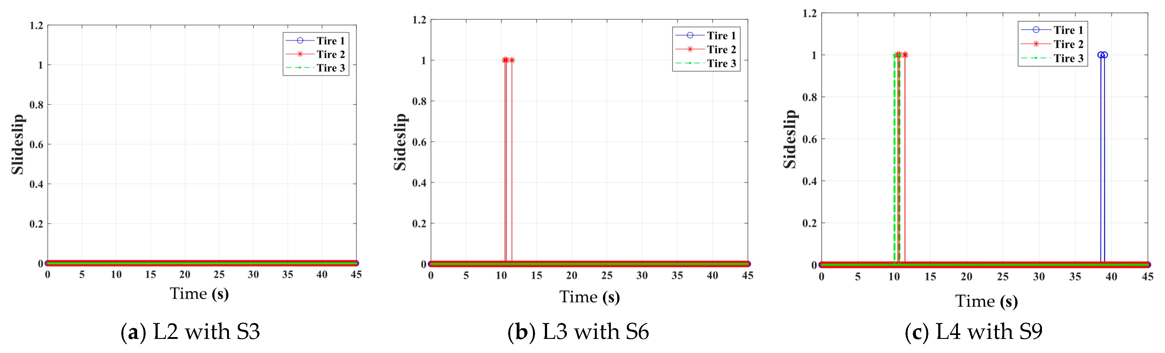
The effects of sea condition levels and wind scales on the traction dynamics of shipboard aircraft are investigated. With increasing sea conditions and wind scales, the front winch rope force becomes more complex, the maximum lateral deformation and force in the tires increase, and the differences in average lateral deformation and force among the tires increase. The stability and safety of winch traction for shipboard aircraft are significantly reduced, particularly when the sea condition level exceeds 3 and the wind scale exceeds 6, leading to a higher risk of tire sideslip or off-ground events.

(4)

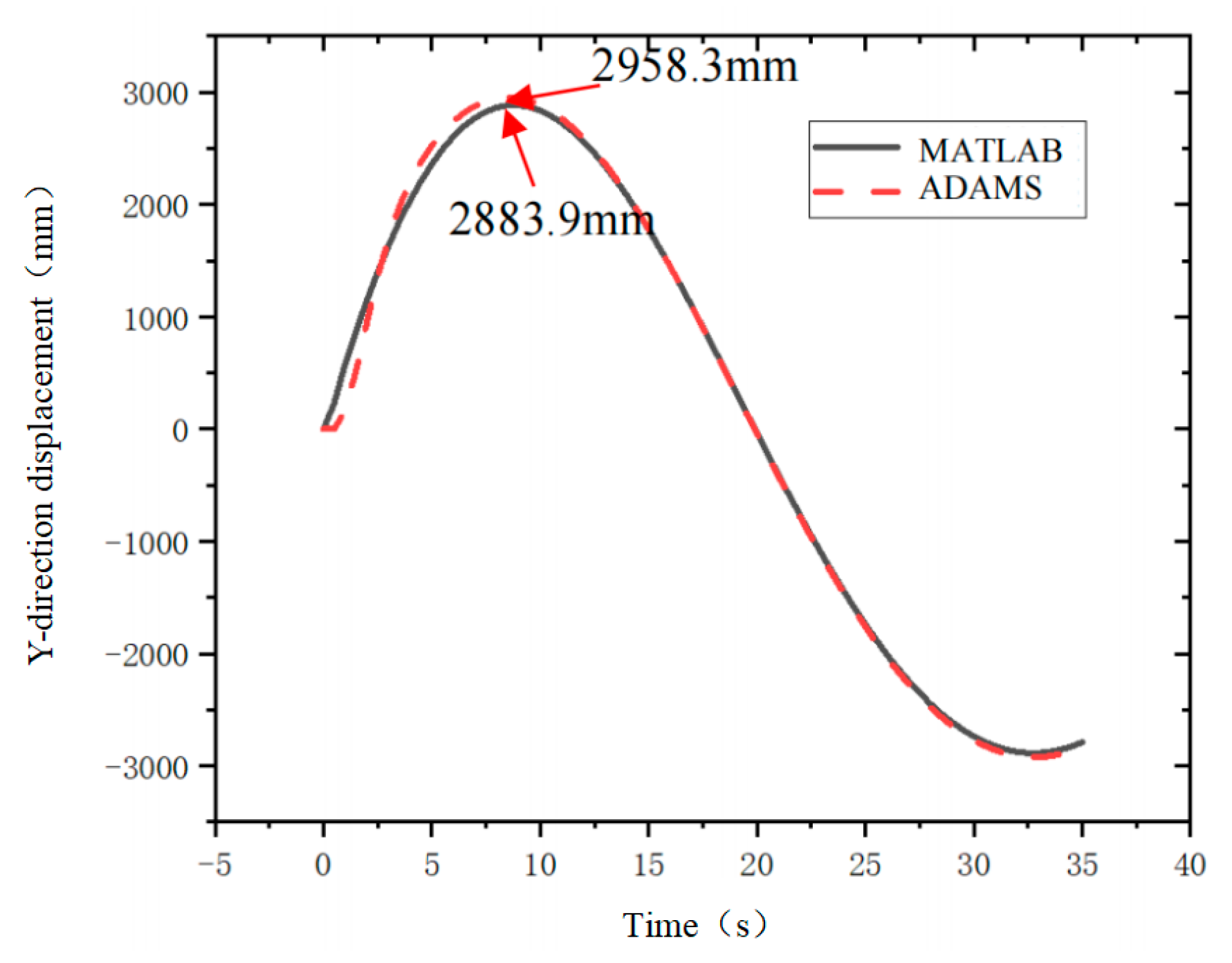
The accuracy of the theoretical calculation method for the winch traction system in this study was verified by conducting multibody dynamics simulations using ADAMS software, with simulation parameters consistent with the theoretical model. The results show that the aircraft towing trajectory and the front winch rope force closely match the MATLAB theoretical calculations, with a maximum error of about 7%. The error in the lateral tire forces is also within acceptable limits. The consistency between simulation and theoretical results confirms the reliability and engineering applicability of the established model.

References

1. Liu, H.; Yang, X.; Li, Y.; Guo, H. Adaptive Backstepping Controller to Improve Handling Stability of Tractor-Aircraft System on Deck. In Proceedings of the 2018 15th International Conference on Ubiquitous Robots (UR), Honolulu, HI, USA, 26–30 June 2018; IEEE: Honolulu, HI, USA, 2018; pp. 839–846. [Google Scholar] [CrossRef]
2. Wang, N.; Liu, H.; Yang, W. Path-tracking control of a tractor-aircraft system. J. Mar. Sci. Appl. 2012, 11, 512–517. [Google Scholar] [CrossRef]
3. Zhao, D.X.; Zhao, Y.; Li, Y.J. Modeling and Simulation of Tractor and Aircraft Multibody System. Adv. Mater. Res. 2012, 466–467, 640–644. [Google Scholar] [CrossRef]
4. Wang, N.J.; Zhou, L.J.; Song, Q.; Zhang, D.F. Simulation Research on Braking Safety Properties of Aircraft Traction System. Key Eng. Mater. 2009, 419–420, 705–708. [Google Scholar] [CrossRef]
5. Jiang, Y.; Feng, G.; Liu, P.; Yuan, L.; Ding, J.; Jiang, B. Influence of Nose Landing Gear Torsional Damping on the Stability of Aircraft Taxiing Direction. Aerospace 2022, 9, 729. [Google Scholar] [CrossRef]
6. Linn, D.R.; Langlois, R.G. Development and Experimental Validation of a Shipboard Helicopter On-Deck Maneuvering Simulation. J. Aircr. 2006, 43, 895–906. [Google Scholar] [CrossRef]
7. Huang, M. Research on loads applied on powered wheels and struts of civil aircraft at touchdown. Proc. Inst. Mech. Eng. Part C J. Mech. Eng. Sci. 2022, 236, 840–851. [Google Scholar] [CrossRef]
8. He, B.; Wang, W.; Zhang, Y.; Liu, L. A Simulation Model of a Helicopter Landing on a Ship. Int. J. Simul. Syst. Sci. Technol. 2016, 17, 5.1–5.7. [Google Scholar] [CrossRef]
9. Thota, P.; Krauskopf, B.; Lowenberg, M.; Coetzee, E. Nonlinear Analysis of the Influence of Tire Inflation Pressure on Nose Landing Gear Shimmy. In Proceedings of the AIAA Modeling and Simulation Technologies Conference, American Institute of Aeronautics and Astronautics, Chicago, IL, USA, 10–13 August 2009. [Google Scholar] [CrossRef]
10. Daniels, N. A Method for Landing Gear Modeling and Simulation with Experimental Validation; NASA: Hampton, VA, USA, 1996.
11. Zhou, C.; Liu, H.; Yang, X.; Han, W. Driving stability control of the carrier-borne aircraft traction system. In Proceedings of the 2022 IEEE International Conference on Real-Time Computing and Robotics (RCAR), Guiyang, China, 17–22 July 2022; IEEE: Guiyang, China, 2022; pp. 355–359. [Google Scholar] [CrossRef]
12. Qi, J.; Xu, H.; Su, M. Study on lateral stability control of carrier-based aircraft towbarless tractor system. Syst. Sci. Control. Eng. 2024, 12, 2343306. [Google Scholar] [CrossRef]
13. Yoo, B.-W.; Park, K.-P.; Oh, J. Dynamics simulation model for the analysis of aircraft movement characteristics on an aircraft carrier deck. Int. J. Nav. Arch. Ocean Eng. 2024, 16, 100591. [Google Scholar] [CrossRef]
14. Liu, J.; Han, W.; Peng, H.; Wang, X. Trajectory planning and tracking control for towed carrier aircraft system. Aerosp. Sci. Technol. 2019, 84, 830–838. [Google Scholar] [CrossRef]
15. Yu, M.; Gong, X.; Fan, G.; Zhang, Y. Trajectory Planning and Tracking for Carrier Aircraft-Tractor System Based on Autonomous and Cooperative Movement. Math. Probl. Eng. 2020, 2020, 1–24. [Google Scholar] [CrossRef]
16. Wang, X.-W.; Peng, H.-J.; Liu, J.; Dong, X.-Z.; Zhao, X.-D.; Lu, C. Optimal control based coordinated taxiing path planning and tracking for multiple carrier aircraft on flight deck. Def. Technol. 2022, 18, 238–248. [Google Scholar] [CrossRef]
17. Su, X.; Li, Z.; Song, J.; Wang, L. A Path Planning Method for Carrier Aircraft on Deck Combining Artificial Experience and Intelligent Search. In Proceedings of the 4th Annual International Workshop on Materials Science and Engineering (IWMSE2018), Xi’an, China, 18–20 May 2018; Volume 381, p. 012194. [Google Scholar] [CrossRef]
18. Marantos, P.; Bechlioulis, C.P.; Kyriakopoulos, K.J. Robust Trajectory Tracking Control for Small-Scale Unmanned Helicopters with Model Uncertainties. IEEE Trans. Control. Syst. Technol. 2017, 25, 2010–2021. [Google Scholar] [CrossRef]
19. Raptis, I.A.; Valavanis, K.P.; Vachtsevanos, G.J. Linear Tracking Control for Small-Scale Unmanned Helicopters. IEEE Trans. Control. Syst. Technol. 2012, 20, 995–1010. [Google Scholar] [CrossRef]
20. Wu, Y.; Qu, X. Obstacle avoidance and path planning for carrier aircraft launching. Chin. J. Aeronaut. 2015, 28, 695–703. [Google Scholar] [CrossRef]
21. Wang, N.; Liu, H. Research on trajectory tracking behavior in traction task for tractor-aircraft system. In Proceedings of the 2013 IEEE International Conference on Mechatronics and Automation, Takamatsu, Japan, 4–7 August 2013; IEEE: Takamatsu, Japan, 2013; pp. 1251–1255. [Google Scholar] [CrossRef]
22. Yu, L.; Huang, M.M.; Jiang, S.; Wang, C.; Wu, M. Unmanned aircraft path planning for construction safety inspections. Autom. Constr. 2023, 154, 105005. [Google Scholar] [CrossRef]
23. Woo, J.W.; An, J.-Y.; Cho, M.G.; Kim, C.-J. Integration of path planning, trajectory generation and trajectory tracking control for aircraft mission autonomy. Aerosp. Sci. Technol. 2021, 118, 107014. [Google Scholar] [CrossRef]
24. Wang, X.; Liu, J.; Su, X.; Peng, H.; Zhao, X.; Lu, C. A review on carrier aircraft dispatch path planning and control on deck. Chin. J. Aeronaut. 2020, 33, 3039–3057. [Google Scholar] [CrossRef]
25. Pritchard, J. Overview of Landing Gear Dynamics. J. Aircr. 2001, 38, 130–137. [Google Scholar] [CrossRef]
26. Yang, H.; Ni, T.; Wang, Z.; Wang, Z.; Zhao, D. Dynamic modeling and analysis of traction operation process for the shipboard helicopter. Aerosp. Sci. Technol. 2023, 142, 108661. [Google Scholar] [CrossRef]
27. Hu, G.; Wu, J.; Qin, X. A novel extension of the Bézier model and its applications to surface modeling. Adv. Eng. Softw. 2018, 125, 27–54. [Google Scholar] [CrossRef]
28. The MathWorks, MATLAB, Version R2021a; The MathWorks Inc.: Natick, MA, USA, 2021. Available online: https://www.mathworks.com (accessed on 1 January 2021).
29. MSC Software, ADAMS, Version 2020; MSC Software Corporation: Newport Beach, CA, USA, 2020. Available online: https://www.mscsoftware.com/product/adams (accessed on 1 January 2020).
Figure 1. Schematic diagram of shipboard aircraft towing methods. (a) tractor traction [2]; (b) winch traction.
Aerospace 12 00579 g001
Figure 2. Force analysis of rope on capstan.
Aerospace 12 00579 g002
Figure 3. Rope model.
Aerospace 12 00579 g003
Figure 4. Schematic diagram of the telescopic landing gear–tire system.
Aerospace 12 00579 g004
Figure 5. Coordinate system of ship motions.
Aerospace 12 00579 g005
Figure 6. Wind load of the ship.
Aerospace 12 00579 g006
Figure 7. Coordinate system of multibody dynamics.
Aerospace 12 00579 g007
Figure 8. Cardan angles.
Aerospace 12 00579 g008
Figure 9. Principle diagram of PID control.
Aerospace 12 00579 g009
Figure 10. The schematic diagram of the third-order Bezier curve.
Aerospace 12 00579 g010
Figure 11. Setting trajectory diagram.
Aerospace 12 00579 g011
Figure 12. Rope force of the front winch.
Aerospace 12 00579 g012
Figure 13. Forces of landing gears and tires.
Aerospace 12 00579 g013
Figure 14. Curves of displacement, velocity, and Euler angle of aircraft centroid over time.
Aerospace 12 00579 g014
Figure 15. Comparison of the lateral forces of tire 3 under the different rear winch positions.
Aerospace 12 00579 g015
Figure 16. Comparison of different towing trajectories.
Aerospace 12 00579 g016
Figure 17. Comparison of aircraft centroid velocity under the different trajectories.
Aerospace 12 00579 g017
Figure 18. Comparison of rope forces of front winch under the different trajectories.
Aerospace 12 00579 g018
Figure 19. Comparison of rope force for the front winch under different sea condition levels and wind scales.
Aerospace 12 00579 g019
Figure 20. Lateral deformation of aircraft tires.
Aerospace 12 00579 g020
Figure 21. Lateral force of aircraft tires.
Aerospace 12 00579 g021
Figure 22. Sideslip situation for the tires of the aircraft.
Aerospace 12 00579 g022
Figure 23. Off-ground situation for the tires of the aircraft.
Aerospace 12 00579 g023
Figure 24. Tricycle-type helicopter model and detailed view of the landing gear.
Aerospace 12 00579 g024
Figure 25. Winch model.
Aerospace 12 00579 g025
Figure 26. Simulation of five-winch traction of aircraft.
Aerospace 12 00579 g026
Figure 27. Comparison between theoretical and actual trajectories.
Aerospace 12 00579 g027