RBF-Learning-Based Many-Objective Metaheuristic for Robust and Optimal Controller Design in Fixed-Structure Heading Autopilot

Abstract

This paper presents an innovative many-objective metaheuristic (MnMH) algorithm designed to tackle the challenges of robust and optimal controller design for fixed-structure heading autopilots. The proposed approach leverages the radial basis function (RBF)-learning operator during the reproduction phase of the MnMH to generate high-quality solutions. A key feature of the method is its generation of a target Pareto front, in which a z-surrogate model makes predictions to guide design solutions toward achieving optimal performance. The effectiveness of the new algorithm is validated through both fixed-structure heading autopilot controller design problems and standard benchmark optimization problems. Results consistently show that the proposed algorithm outperforms several existing MnMHs across all tested scenarios. This study offers valuable insights into many-objective optimization and demonstrates the algorithm’s potential for enhancing robust controller design in heading autopilot systems.

1. Introduction

Aviation is a cornerstone of modern life. Advancements are increasingly pushing the performance boundaries of autonomous unmanned aerial vehicles (UAVs). These pilotless systems are revolutionizing industries by performing tasks in agriculture, mapping, military operations, surveying, and other fields [1,2,3,4]. Their ability to operate in hazardous environments has fueled global research into UAV design, particularly in trajectory and path optimization to ensure optimal mission performance. With no onboard pilots, UAV control systems must exhibit exceptional trajectory tracking and robustness to uncertainties and disturbances across diverse flight conditions [5].

Designing effective flight control systems involves addressing a complex many-objective optimization challenge. Traditional methods, such as root locus [6] and loop shaping [7], struggle to meet modern performance and robustness demands. Similarly, single-objective approaches like the linear–quadratic regulator (LQR) [8] and linear–quadratic–Gaussian (LQG) [9] fall short of simultaneously satisfying all design requirements. While advanced techniques such as H-infinity control [10] and Mu-synthesis [11] provide robust solutions, they rely on the experience-driven tuning of weighting factors [12] and often lead to high-order controllers, making practical implementation difficult.

Fixed-structure controllers offer a more feasible alternative due to their simplicity, interpretability, and ease of implementation [13]. However, their design requires solving non-convex, constrained optimization problems [14,15]. Conventional non-smooth optimization methods [16], though widely applied, become inefficient as constraints increase and they are prone to converging on local optima. In contrast, metaheuristic algorithms (MHs), including genetic algorithms [17], particle swarm optimization [18], and differential evolution [19], have demonstrated flexibility and effectiveness in tackling complex control design challenges [20,21]. Recent studies, including our own, have highlighted the potential of MHs for optimizing fixed-structure flight controllers, particularly in UAV applications [22].

A key advantage of MHs is their ability to pose control design as a constrained many-objective optimization problem. Many-objective metaheuristics (MnMHs) can generate Pareto-optimal solutions in a single run, enabling simultaneous optimization of multiple design objectives [23]. However, despite their potential, MnMHs often face challenges in search consistency and convergence, especially when dealing with more than three objectives [24,25]. Most existing research [26] has primarily focused on improving control performance for fixed-structure flight control systems while overlooking robustness to disturbances and uncertainties. Given the critical role of robustness in practical applications, there remains a significant gap in achieving reliable controller designs that effectively balance multiple objectives.

The current study proposes a novel MnMH algorithm tailored for robust fixed-structure heading autopilot controller optimization to bridge this critical gap. This approach seeks to improve both performance and robustness while addressing the limitations of existing methods.

Our approach integrates an RBF-learning operator during the MnMH reproduction phase to generate high-quality solutions. This study aims to achieve two primary objectives: (1) to develop a framework for optimizing robust fixed-structure heading autopilot controller design with four critical objectives, and (2) to propose an efficient MnMH algorithm to solve this optimization problem. The proposed method incorporates a self-adaptive multi-objective real-coded population-based incremental learning hybridized with differential evolution (A-MRPBIL-DE) algorithm [27], utilizing iterative parameter distribution estimation. Additionally, an RBF-learning operator is presented to enhance search convergence and ensure consistency.

The proposed algorithm’s performance is evaluated on benchmark test problems and a robust controller design task for fixed-structure heading autopilots. Comparative analysis with established MnMHs demonstrates superior performance across key metrics, including hypervolume (HV), generational distance (GD), inverted generational distance (IGD), and spacing-to-extent (STE). Statistical analyses further validate the algorithm’s effectiveness, showcasing its potential as a robust solution for modern UAV control challenges.

2. Formulation of the Robust Optimal Fixed-Structure Heading Autopilot Design Problem

2.1. UAV Model Utilized in This Study

In this study, we address the design challenge of develsoping a robust and optimal fixed-structure heading autopilot for the Hawkeye UAV. Specifically, we focus on creating a flight controller for heading control. Figure 1 illustrates the notation used to describe the linear and rotational velocities acting on the aircraft. The Hawkeye UAV is a prototype developed by the Department of Aerospace Engineering at the University of Kansas [28]. Detailed specifications for the UAV, along with its lateral linear state-space model, can be found in the MATLAB code provided in Appendix B in [28].

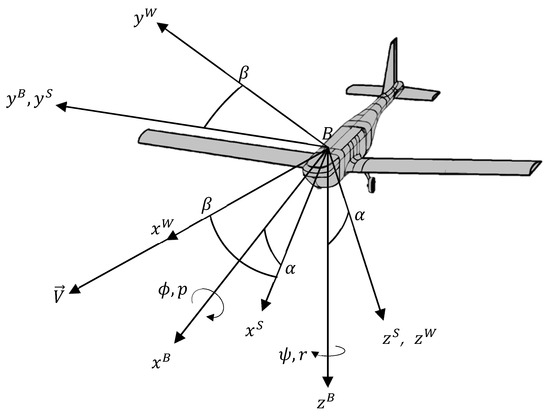
Figure 1. Notation for linear and rotational velocities in the body axis system. The origin of coordinates is at the vehicle’s center of mass.

The lateral linear state-space model isolates the lateral/directional dynamics by assuming that longitudinal variables remain decoupled under small perturbations about steady-level flight. As presented in Equation (1), the model comprises five state variables: sideslip angle (β), roll rate (p), roll angle (ϕ), yaw rate (r), and yaw angle (ψ), collectively denoted as $\mathit{x}={\left\{\beta ,p,\varphi ,r,\psi \right\}}^T$. The control inputs are the aileron deflection (${\mathsf{\delta }}_{\mathrm{a}}$) and rudder deflection (${\mathsf{\delta }}_{\mathrm{r}}$), represented as $\mathit{u}={\{{\delta }_a , {\delta }_r\}}^T$. The system has been verified to be fully controllable and observable. Additionally, all eigenvalues of the system matrix $\mathit{A}$ lie in the left half of the complex plane, confirming the open-loop stability of the system.

The output vector is $\mathbf{y}={\left\{p,\varphi ,r,\psi \right\}}^T$. In practical applications, the sideslip angle $\beta$ is not directly measurable but can be estimated using observer-based methods such as the Kalman filter. In this study, however, all state variables are assumed to be accurately measured.

$$\begin{array}{cc}\dot{\mathit{x}} =& \mathit{A}\mathit{x}+\mathit{B}\mathit{u}\hfill \\ \mathit{y} =& \mathit{C}\mathit{x}\hfill \end{array}$$

(1)

where

$$\begin{gathered} \mathit{A}=\left[\begin{array}{ccccc}-0.216& 0.358& -0.005& -0.994& 0\\ 0& 0& 1& 0.009& 0\\ -15.763& 0& -12.964& 3.003& 0\\ 14.080& 0& -5.883& -0.594& 0\\ 0& 0& 0& 1& 0\end{array}\right], \mathit{B}=\left[ \begin{array}{cc}0& 0.122\\ 0& 0\\ 59.154& -6.558\\ 5.930& -29.988\\ 0& 0\end{array} \right], \\ \mathrm{and} \mathit{C}=\left[\begin{array}{ccccc}0& 0& 0& 0& 0\\ 0& 1& 0& 0& 0\\ 0& 0& 1& 0& 0\\ 0& 0& 0& 1& 0\\ 0& 0& 0& 0& 1\end{array}\right] \end{gathered}$$

2.2. Robust Optimum Fixed-Structure Heading Autopilot Design Approach

The heading autopilot controller in this study follows the control structure shown in Figure 2, with the synthesized controllers labeled as $K_{\psi }$, $K_{ \varphi }$, $K_p,$ and $K_r$. Typically, $K_{\psi }$, $K_p,$ and $K_r$ function as proportional (P) controllers, while $K_{ \varphi }$ is implemented as a proportional–integral (PI) controller. The formulation of $K_{\psi }$, $K_{ \varphi }$, $K_p,$ and $K_r$ is defined as follows:

$$K_{\psi }={K_{\psi }}_P , K_{ \varphi }={\displaystyle \frac{{K_{ \varphi }}_{P}s+{K_{ \varphi }}_I}{s}} , K_p={K_p}_P \mathrm{a}\mathrm{n}\mathrm{d} K_r={K_r}_P.$$

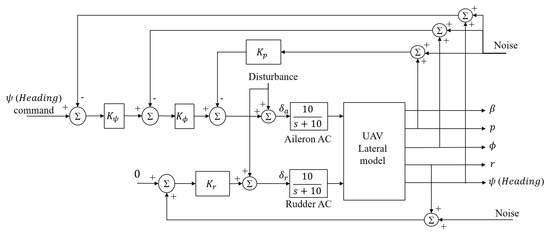
Figure 2. Flight control system model.

An optimization problem is formulated to identify controllers that simultaneously optimize multiple performance criteria, including handling perturbations and uncertainties, disturbance attenuation, noise rejection, and minimizing control energy to achieve a robust and optimal heading autopilot controller. The overall autopilot system is illustrated in Figure 2, while Figure 3 presents a simplified block diagram of the control system, incorporating plant model uncertainties, with the following variables:

• ${\mathit{r}=\left\{\begin{array}{cccc}0& 0& 0& {\psi }_{command}\end{array}\right\}}^T$ is the input signal,
• ${\mathit{y}=\left\{p \varphi r \psi \right\}}^T$ is the output signal,
• $\mathit{K}=\left[\begin{array}{cccc}{K}_p& K_{ \varphi }& 0& K_{ \varphi }{K}_{\psi }\\ 0& 0& -K_r& 0\end{array}\right]$ are flight controllers,
• ${\mathit{u}=\left\{\begin{array}{cc}{\delta }_a& {\delta }_r\end{array}\right\}}^T$ is the control signal,
• G = plant model, which includes an actuator, and,
• Δ = additive perturbation or uncertainty in the plant model.

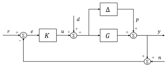
Figure 3. A closed-loop configuration of [G] and [K].

The relationship between the input signal (r), output signal (y), control signal (u), error signal (e), disturbance (d), measurement noise (n), and perturbation (p) can be expressed as follows:

$$\begin{gathered} \mathit{y}={\left[\mathit{I}+\mathit{G}\mathit{K}\right]}^{-1}\mathit{G}\mathit{K}\mathit{r}+{\left[\mathit{I}+\mathit{G}\mathit{K}\right]}^{-1}\mathit{G}\mathit{d}-{\left[\mathit{I}+\mathit{G}\mathit{K}\right]}^{-1}\mathit{G}\mathit{K}\mathit{n}-{\left[\mathit{I}+\mathit{G}\mathit{K}\right]}^{-1}\mathit{G}\mathit{K}\mathit{p} \\ \mathit{u}={\left[\mathit{I}+\mathit{K}\mathit{G}\right]}^{-1}\mathit{K}\mathit{r}-{\left[\mathit{I}+\mathit{K}\mathit{G}\right]}^{-1}\mathit{K}\mathit{G}\mathit{d}-{\left[\mathit{I}+\mathit{K}\mathit{G}\right]}^{-1}\mathit{K}\mathit{n}-{\left[\mathit{I}+\mathit{K}\mathit{G}\right]}^{-1}\mathit{K}\mathit{p} \\ \mathit{e}={\left[\mathit{I}+\mathit{G}\mathit{K}\right]}^{-1}\mathit{r}-{\left[\mathit{I}+\mathit{G}\mathit{K}\right]}^{-1}\mathit{G}\mathit{d}-{\left[\mathit{I}+\mathit{G}\mathit{K}\right]}^{-1}\mathit{n}+{\left[\mathit{I}+\mathit{G}\mathit{K}\right]}^{-1}\mathit{p} \end{gathered}$$

Finding all stabilizing controllers K to minimize the ∞-norm (infinity norm) of the corresponding transfer function matrices is a controller design problem that aims to achieve robust stability and optimal control performance. Achieving these objectives enhances the system’s capability to reject external disturbances while maintaining effective control action. This design goal can be summarized as follows:

• For good reference tracking (r→e)

  $${min:‖{\left[\mathit{I}+\mathit{G}\mathit{K}\right]}^{-1}‖}_{\infty }$$
• For good handling perturbation or uncertainty (p→u)

  $${min:‖-{\left[\mathit{I}+\mathit{K}\mathit{G}\right]}^{-1}\mathit{K}‖}_{\infty }$$
• For good gust disturbance attenuation (d→y)

  $$min:{‖{[\mathit{I}+\mathit{G}\mathit{K}]}^{-1}\mathit{G}‖}_{\infty }$$
• For good noise rejection (n→y)

  $$min:{‖-{\left[\mathit{I}+\mathit{G}\mathit{K}\right]}^{-1}\mathit{G}\mathit{K}‖}_{\infty }$$
• For less control energy (r→u)

  $${min:‖{\left[\mathit{I}+\mathit{K}\mathit{G}\right]}^{-1}\mathit{K}‖}_{\infty }$$

2.3. Optimization Problem for a Robust Many-Objective Fixed-Structure Heading Autopilot Controller Design

In Section 2.2, the design of a flight controller to achieve robustness and optimality requires simultaneous optimization of several objective functions, a task that cannot be accomplished using conventional controller design techniques. While some modern controller design techniques, such as H-infinity and Mu-synthesis, are considered optimal control design methods, they typically involve a single-objective optimization solver. In those approaches, all requirement functions need to be compromised using weighting factors that are intuitively predefined by a designer. This work leverages the advantages of many-objective metaheuristic (MnMH) techniques to address this challenge. By employing a many-objective optimization approach, MnMHs simultaneously optimize all requirements in both robustness and performance, providing a more comprehensive solution to the controller design problem.

The optimization problem is formulated to identify all possible controllers, as depicted in Figure 2, defined as $\mathit{x}={\left\{{K_{\psi }}_P, {K_{ \varphi }}_P, {K_{ \varphi }}_I, {K_p}_P, {K_r}_P\right\}}^T,$ where $0<\mathbf{x}<100.$ This is performed to minimize many-objective functions for optimal reference tracking, effective perturbation or uncertainty handling, robust gust disturbance attenuation, efficient noise rejection, and reduced control energy, subject to several constraints. The formulation of the proposed optimization problem is expressed as follows:

$$min:\mathit{f}(\mathit{x})={\left\{f_1\left(\mathit{x}\right),f_2\left(\mathit{x}\right),f_3(\mathit{x}),f_4(\mathit{x})\right\}}^T$$

Subjected to:

$g_1\left(\mathit{x}\right)=\max ({\lambda }_A)<0$,	$g_7\left(\mathit{x}\right)=p\le 40 {\displaystyle \frac{deg}{s}},$
$g_2\left(\mathit{x}\right)=\mathit{settling} \mathit{time}\le 30 \mathit{s}$,	$g_8\left(\mathit{x}\right)=\varphi \le 40 deg$,
$g_3\left(\mathit{x}\right)=\%\mathit{overshoot}\le 5\%$,	$g_9\left(\mathit{x}\right)=r\le 20 {\displaystyle \frac{deg}{s}}$,
$g_4\left(\mathit{x}\right)=\mathit{rise} \mathit{time}\le 15 s$,	$g_{10}\left(\mathit{x}\right)={\delta }_a\le 30 deg$,
$g_5\left(\mathit{x}\right)=\%\left|\left.{\psi }_{t_{\infty }}-{\psi }_{ref}\right|\right.\le 2\%$,	$g_{11}\left(\mathit{x}\right)={\delta }_r\le 30 deg$,
$g_6\left(\mathit{x}\right)=\beta \le 20 deg,$

where

$f_1\left(\mathit{x}\right)={\int }_{t=0}^t{e}_{\psi }^2\left(t\right)dt$	To achieve accurate heading reference tracking.
$f_2\left(\mathit{x}\right)={‖-{\left[\mathit{I}+\mathit{K}\mathit{G}\right]}^{-1}\mathit{K}‖}_{\mathit{\infty }}$	To effectively handle perturbations or uncertainties while minimizing control energy.
$f_3\left(\mathit{x}\right)={‖{[\mathit{I}+\mathit{G}\mathit{K}]}^{-1}\mathit{G}‖}_{\infty }$	For effective attenuation of gust disturbances.
$f_4\left(\mathit{x}\right)={‖-{\left[\mathit{I}+\mathit{G}\mathit{K}\right]}^{-1}\mathit{G}\mathit{K}‖}_{\infty }$	For effective noise rejection.

The f₁(x) represents the integral squared error of the heading step response, aiming for optimal reference tracking. Concurrently, functions f₂(x), f₃(x), and f₄(x) are designed for effective perturbation or uncertainty handling, reduced control energy, robust gust disturbance attenuation, and efficient noise rejection, respectively, as detailed in Section 2.2.

The constraint $g_1\left(\mathit{x}\right)$ ensures the stability of the entire control system, with ${\mathit{\lambda }}_A$ representing all eigenvalues of the state matrix (A) in the state equation of the closed-loop control system. Constraints $g_2\left(\mathit{x}\right)$ to $g_4\left(\mathit{x}\right)$ are imposed to facilitate fast reference tracking, while constraint $g_5\left(\mathit{x}\right)$ ensures reference tracking accuracy. Constraints $g_6\left(\mathit{x}\right)$ to $g_{11}\left(\mathit{x}\right)$ are implemented to restrict the response of all state variables and control ability [28].

3. RBF-Learning-Based A-MRPBIL-DE for Many-Objective Optimization

3.1. Self-Adaptive Multi-Objective Real-Code Population-Based Incremental Learning Hybridized with Differential Evolution (A-MRPBIL-DE)

Self-adaptive multi-objective real-code population-based incremental learning hybridized with differential evolution (A-MRPBIL-DE), proposed by Bureerat et al. in 2019 [27], is an improved version of multi-objective real-code population-based incremental learning hybridized with differential evolution (MRPIBL-DE) [29]. MRPIBL-DE was enhanced to become A-MRPBIL-DE by transforming all predefined processing parameters into iterative self-adaptive parameters. Its performance was verified for robot trajectory planning optimization problems. The search procedure of A-MRPBIL-DE consists of four main processes, population initialization, Pareto selection, reproduction, and parameter adaptation. In the A-MRPBIL-DE reproduction process, there are two main reproduction phases, RPBIL reproduction and DE reproduction phases.

For the RPBIL phase, the reproduction process is carried out by updating probability trays used to generate a new population, while Equations (2)–(5) are employed for updating an element in a probability tray (for a more in-depth understanding of this process, please refer to [29]).

$$P_{ijk}^{\prime }=(1-L_R(j))P_{ijk}^{old}+L_R(j)$$

(2)

$$L_R(j)={L_R}_0\mathit{exp}(-(j-r{)}^2)$$

(3)

where P_ij represents the probability of having x_i in the subinterval j of the kth tray. L_R0 is the initial learning rate, and r is the subinterval number where the ith element of the centroid of design variables of each group is located. Then, the updated probability matrix P′_ij is modified as

$$P_{ijk}^{″}=P_{ijk}^{\prime }/{\sum }_{j=1}^{n_I}{P}_{ijk}^{\prime }$$

(4)

to satisfy the condition

$${\sum }_{j=1}^{n_I}{P}_{ijk}^{″}=1$$

(5)

where P″_ijk is the final update of P_ijk.

For the DE phase, the new population generated from the RPBIL phase is reproduced again through a specially proposed DE reproduction process [29], involving mutation and crossover. The DE mutation process is executed based on Equation (6), expressed as:

$${\mathit{x}}_i^{new}=\left\{\begin{array}{c}{\mathit{x}}^{best}+F\left({\mathit{x}}_1^r-{\mathit{x}}_2^r\right); if rand<P_{Mu} \\ {\mathit{x}}^{best}+F\left({\mathit{x}}_1^r+{\mathit{x}}_2^r-{\mathit{x}}_3^r-{\mathit{x}}_4^r\right); otherwise\end{array}\right.$$

(6)

where F is a scaling factor and ${\mathit{x}}^{best}$ is the best individual in the current population. In the multi-objective version, the ${\mathit{x}}^{best}$ in Equation (6) is a randomly selected solution in the Pareto archive. The ${\mathit{x}}_i^r$ are four randomly selected individuals from the current population, X, or from a Pareto archive, A, based on a probability P_xr, expressed as follows:

$${\mathbf{x}}_i^r\in \left\{\begin{array}{c}\mathit{X} ; if rand<P_{Xr} \\ \mathit{A}; otherwise \end{array}\right.$$

After finishing the mutation process, for a new individual ${\mathit{x}}^{new}=\left\{x_1^{new},\dots ,x_D^{new}\right\}$ and an old individual ${\mathbf{x}}^{old}=\left\{x_1^{old},\dots ,x_D^{old}\right\}$, the DE binomial crossover process is performed based on Equation (7), expressed as follows:

$$x_j^{new}=x_j^{old}; if rand<CR, for j=1,\dots ,D$$

(7)

where rand is a uniform random number in the range [0,1], CR and D are the crossover rate and the number of design variables, respectively. For all processing parameters, P_Mu, P_xr, P_c, F, and CR, in each calculation, the parameters P_Mu, P_xr, and CR are generated by means of normal distribution randomization [30,31,32] based on their mean values, P_Mum, P_xrm, and CR_m. The parameter F is generated by using a Lehmer mean value [30,31,32] based on its mean values, F_m, and a standard deviation of 0.1. For each iteration, the parameters P_Mum, P_xrm, F_m, and CR_m are iteratively self-adaptive using Equations (8)–(11).

P_Mum(T + 1) = 0.9P_Mum (T) + 0.1mean(good_PMu),

(8)

P_xrm(T + 1) = 0.9P_xrm (T) + 0.1mean(good_Pxr),

(9)

CR_m(T + 1) = 0.9CR_m(T) + 0.1mean(good_CR),

(10)

$$F_m(T+1)=0.9F_m(T)+0.1{\displaystyle \frac{sum(goo{d}_F^2)}{sum(goo{d}_F)}}$$

(11)

where good_PMu, good_Pxr, good_CR, and good_F are archives collecting the values of P_Mu, P_xr, F, and CR, which have been successfully used for generating a new solution. Successfully generated solutions are those that dominate a solution in the Pareto archive (A). The function mean(good_X) represents the average value of the members in the archive good_X, while sum(good_F) and sum($goo{d}_F^2$) indicate the summation and sum of squares of all elements in good_F, respectively. In this work, weighting factors of 0.9 and 0.1 in Equations (8)–(11) are chosen based on the successful record, as reported in [30,31,32].

The search procedure for A-MRPBIL-DE is outlined in Algorithm 1. The process begins with initializing probability trays, an empty Pareto archive, initialized values of P_Mum, P_xrm F_m, and CR_m, and empty archives good_PMu, good_Pxr, good_CR, and good_F. The parameters P_Mu, P_xr, F, and CR are then generated, and the real-code population is created through the combination of RPBIL and DE operators. After conducting objective function evaluations, non-dominated solutions are sorted from the combination of the newly generated solutions and the current Pareto archive. For a newly generated solution that dominates one of the members in the Pareto archive, the parameters P_Mu, P_xr, F, and CR used to create this solution are saved to the archives good_PMum, good_Pxrm, good_CR, and good_F. Subsequently, the probability trays, the Pareto archive, and the parameters P_Mum, P_xrm, F_m, and CR_m are iteratively updated using Equations (8)–(11). The search procedure is repeated until a termination criterion is satisfied.

Algorithm 1. A-MRPBIL-DE.

Input: Number of iterations (NG), population size (NP), number of design domain subintervals (nI), number of trays (NT), and Pareto archive size (NA). Output: A Main Procedure Initialization 1: Define Pij = nI/Np for each tray, a Pareto archive A = {}. 2: Generate a real-code population X from the probability trays and evaluate objective function values. 3: Select non-dominated solutions from X∪A and save them to A. 4: Set initial PMum = 0.5, Pxrm = 0.5, Fm = 0.5, CRm = 0.5. 5: Set initial goodPMum = {}, goodPxrm = {}, goodCR = {} and goodF = {}. 6: For i = 1 to NG. Update the population using the RPBIL operation 7: Divide the non-dominated solutions into NT groups using a clustering technique and find the centroid rG of each group. 8: Update the probability trays using rG. 9: Generate a real code population X from the probability trays. Update the population using a DE operation 10: For j = 1 to NP  10.1: Generate PMu, Pxr, and CR by a random normal distribution and generate F   by the Lehmer mean technique.  10.2: Randomly select a solution xbest from Pareto archive A.  10.3: Randomly select four solutions, xr1, xr2, xr3, and xr4.   10.3.1 If rand < Pxr, select the xr1, xr2, xr3, and xr4 from the current population X.   10.3.2 Otherwise, select the xr1, xr2, xr3, and xr4 from Pareto archive A.  10.4: Generate a new solution using the mutation schemes in Equation (6).  10.5: Perform crossover schemes in Equation (7).  10.6: Save the newly generated solution in Y. 11: End. 12: Evaluate objective function values of the new population. Pareto selection 13: Select non-dominated solutions from Y∪A and save as A. For each yi∈Y that dominates at least one solution in A, the parameters, PMu, Pxr, CR, and F index i are saved to goodPMu, goodPxr, goodCR, and goodF, respectively. Processing parameter adaption 14: Update the parameters, PMum, Pxrm Fm, and CRm using Equations (8)–(11). 15: If the number of A is larger than NA, remove some of the members in A using a clustering technique. 16: End.

3.2. RBF-Learning-Based A-MRPBIL-DE

This part represents the main contribution to the metaheuristic search in this paper. An improved version of A-MRPBIL-DE, detailed in Section 3.1, is proposed using the RBF-learning operator. The primary concept is to integrate a learning operator based on the RBF surrogate model into the algorithm’s reproduction process to generate new solutions based on a target front. Typically, the conventional reproduction process generates a new solution without specifically considering the target point or the expected objective function value, but rather expecting that the solution will be improved. This process is termed the forward reproduction process.

An RBF surrogate model is commonly used for objective function estimation in surrogate-based optimization. However, in this work, it is exploited in the opposite manner. The novel proposed idea works differently, where the target points (vectors of objective functions) are defined, and RBF is used to predict a solution that is expected to reach these target points. The RBF model is reconstructed at each iteration based on a set of non-dominated solutions. The details of the proposed method, utilizing the RBF-learning reproduction process to generate a new solution, are expressed as follows:

Given a many-objective optimization problem defined as:

$$\underset{\mathbf{x}}{\min }\mathit{f}\left(\mathit{x}\right)={\left\{f_1,\dots ,f_M\right\}}^T;{\mathit{x}}^L\le \mathit{x}\le {\mathit{x}}^U.$$

(12)

At a particular loop, a non-dominated front can be written as ${\mathit{F}}_{M\times N}=[{\mathbf{f}}^1,\dots ,{\mathbf{f}}^N]$ with the corresponding design solutions.

$${\mathit{X}}_{\mathit{n}\times \mathit{N}}=[{\mathbf{x}}^1,\dots ,{\mathbf{x}}^N]$$

(13)

The concept of exploiting RBF for metaheuristic search in this work is contrary to conventional surrogate-assisted optimization, as ${\mathit{F}}_{M\times N}$ is assigned as a set of training points while the function values are ${\mathit{X}}_{n\times N}$. In the RBF-learning operator, a solution can be estimated using a radial basis function based on Equation (14).

$$\mathit{x}{\left({\overline{\mathit{f}}}^i\right)}_{n\times 1}={\sum }_{i=1}^N{\mathit{c}}^{i}K\left(\left|\left|\mathit{f}-{\overline{\mathit{f}}}^i\right|\right|\right)={\mathit{C}}_{n\times N}{\left\{K\left(\left|\left|\mathit{f}-{\overline{\mathit{f}}}^i\right|\right|\right)\right\}}_{N\times 1}$$

(14)

where C is a matrix of coefficients, determined as follows:

$$\mathit{C}=\left\{{\mathit{c}}^1,\dots ,{\mathit{c}}^N\right\}=\mathit{X}{\mathit{A}}^{-1}$$

(15)

where

$${\mathit{A}}_{ij}=\left[K_n\left(\left|\left|{\mathbf{f}}^i-{\mathbf{f}}^j\right|\right|\right)\right].$$

(16)

K(x) is an RBF kernel function of x. Then, a target point to improve a particular solution in the non-dominated front, as shown in Figure 4, can be defined as

$${\overline{\mathit{f}}}^i={\mathit{f}}^i+\mathit{\delta }$$

(17)

where a choice for δ can be a normal vector of the hyperplane generated from the anchor points (u_i) of the current non-dominated front. Having obtained the target value in (17), it is then substituted into (14) to obtain an approximate solution. The simplest way to deal with the modification in (17) is to initially transform the objective function domain to a normalized domain using the relation

$$f_i^{\prime }={\displaystyle \frac{f_i-f_i^{Min}}{f_i^{Max}-f_i^{Min}}}$$

(18)

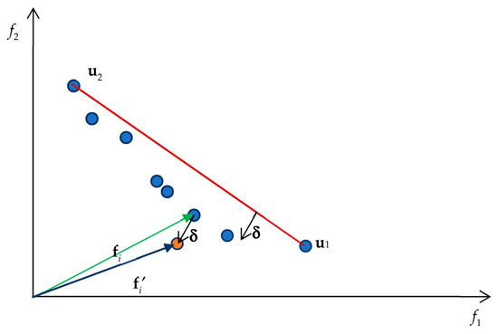
Figure 4. Original domain.

With the mapping in (18), the anchor point of the ith objective function will have its ith element as one, while the rest are zeros (Figure 5). The hyperplane equation can be expressed as:

$$f_1^{\prime }+\dots +f_M^{\prime }=1$$

(19)

which means the normal vector is:

$${\mathit{\delta }}^{\prime }=-1.$$

(20)

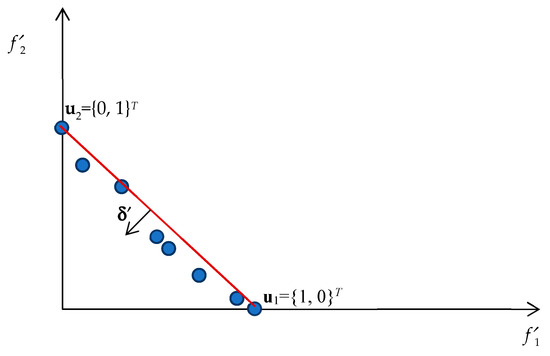
Figure 5. Normalized domain.

In cases where we need to slightly change the target function from its original function value, the vector ${\mathbf{\delta }}^{\prime }$ may be defined as

$${\mathit{\delta }}^{\prime }=-ϵ1.$$

(21)

where $ϵ$ is a predefined small number. If we want to make it more random, which tends to be more diverse for a metaheuristic, the vector can be defined as:

$$\left\{{{\delta }^{\prime }}_i\right\}=\{-ϵ.ran{d}_i\}$$

(22)

where $rand\in \left[\mathrm{0,1}\right]$ is a uniform random number. Then, the function in the normalized domain can be modified as

$$\widehat{\mathit{f}}={\mathit{f}}^{\prime }+{\mathit{\delta }}^{\prime }$$

(23)

Afterward, it can be mapped to the original function domain ${\overline{\mathit{f}}}^i$ using Equation (18). In conclusion, the newly proposed metaheuristic reproduction operator starts with generating a pseudo non-dominated front from the current loop information as in Equation (23). Then, the RBF-learning technique with additional randomization is applied to create design solutions.

An example of using the RBF-learning operator for the reproduction of design solutions can be expressed in Example 1.

Example 1.

RBF-learning operator to generate new solutions.

Consider the bi-objective optimization problem given by:

$$\min :{\{f}_1\left(\mathit{x}\right)=x_1^2+x_2^2, f_2\left(\mathit{x}\right)={\left(x_1-1\right)}^2+{\left(x_2-2\right)}^2)\}$$

At the current iteration, the set of design solutions is:

$$\mathit{x}=\left\{\begin{array}{c}{x}_1\\ x_2\end{array}\right\}=\left\{\begin{array}{cccccccccc}0.3361& 0.0049& 0.7661& 0.6397& 0.6963& 0.2158& 0.9731& 0.9532& 0.3472& 0.1284\\ 0.9811& 0.9899& 0.3635& 0.0288& 0.1869& 0.7975& 0.0581& 0.6424& 0.5929& 0.2908\end{array}\right\}$$

Then, the corresponding set of objective function values is:

$$\{\mathit{f}\}=\left\{\begin{array}{c}{f}_1\\ f_2\end{array}\right\}=\left\{\begin{array}{cccccccccc}1.0755& 0.9799& 0.7190& 0.4100& 0.5198& 0.6826& 0.9503& 1.3213& 0.4721& 0.1011\\ 1.4789& 2.0105& 2.7328& 4.0154& 3.3796& 2.0610& 3.7717& 1.8453& 2.4061& 3.6811\end{array}\right\}$$

The non-dominated solutions are shown below. Figure 6 provides a plot of all the design solutions on the objective function domain, where the non-dominated solutions are the black markers.

$${\{\mathit{f}}_{\mathrm{n}\mathrm{o}\mathrm{n}-\mathrm{d}\mathrm{o}\mathrm{m}\mathrm{i}\mathrm{n}\mathrm{a}\mathrm{t}\mathrm{e}\mathrm{d}}\}=\left\{\begin{array}{ccccc}1.0755& 0.9799& 0.6826& 0.4721& 0.1011\\ 1.4789& 2.0105& 2.0610& 2.4061& 3.6811\end{array} \right\}$$

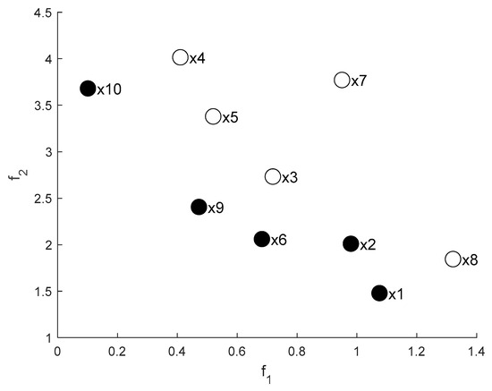
Figure 6. Current solutions and the current Pareto front.

The normalized non-dominated solution, ${\{\mathit{f}}_{\mathrm{n}\mathrm{o}\mathrm{n}-\mathrm{d}\mathrm{o}\mathrm{m}\mathrm{i}\mathrm{n}\mathrm{a}\mathrm{t}\mathrm{e}\mathrm{d}}^{\prime }\}$ is then given by:

$$\{{\mathit{f}}_{\mathrm{n}\mathrm{o}\mathrm{n}-\mathrm{d}\mathrm{o}\mathrm{m}\mathrm{i}\mathrm{n}\mathrm{a}\mathrm{t}\mathrm{e}\mathrm{d}}^{\prime }\}=\left\{\begin{array}{ccccc}1.0000& 0.9019& 0.5968& 0.3807& 0\\ 0& 0.2414& 0.2643& 0.4210& 1.0000\end{array} \right\}$$

Using Equation (22) with $ϵ=0.25$, we have:

$${\mathit{\delta }}^{\prime }=\left\{\begin{array}{ccccc}0.0690& 0.1477& 0.0178& 0.0914& 0\\ 0& 0.0098& 0.0329& 0.0358& 0.0560\end{array} \right\}$$

Applying Equation (23), we obtain:

$$\{\widehat{\mathit{f}}\}=\left\{\begin{array}{ccccc}0.9310& 0.7542& 0.5790& 0.2894& 0\\ 0& 0.2316& 0.2314& 0.3852& 0.9440\end{array} \right\}$$

The transformed function values mapped to the original function domain, using Equation (18), are:

$$\{\overline{\mathit{f}}\}=\left\{\begin{array}{ccccc}1.0083& 0.8360& 0.6653& 0.3831& 0.1011\\ 1.4789& 1.9889& 1.9885& 2.3272& 3.5578\end{array} \right\}$$

Figure 7 illustrates a set of non-dominated solutions and target points. Once the target points are determined, a new solution, {x_new}, corresponding to those target points is approximated using Equation (14):

$${{\mathit{x}}_{\mathit{n}\mathit{e}\mathit{w}}^{\mathit{i}}\left({\overline{\mathit{f}}}^i\right)}_{n\times 1}={\mathit{C}}_{n\times N}{\left\{K\left(\left|\left|\mathit{f}-{\overline{\mathit{f}}}^i\right|\right|\right)\right\}}_{N\times 1}$$

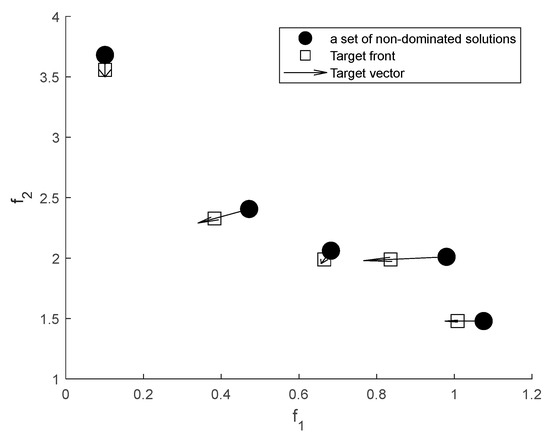
Figure 7. Plot of a set of non-dominated solutions and target points.

The computed new solutions are:

$$\{{\mathit{x}}_{\mathit{n}\mathit{e}\mathit{w}}\}=\left\{\begin{array}{ccccc}0.3043& 0.0932& 0.1784& 0.2987& 0.2049\\ 0.9926& 0.9154& 0.8419& 0.6445& 0.3014\end{array} \right\}$$

while the corresponding real objective function values are:

$$\left\{{\mathit{f}}_{\mathit{n}\mathit{e}\mathit{w}}\right\}=\left\{\begin{array}{ccccc}1.0779& 0.8466& 0.7407& 0.5046& 0.1328\\ 1.4988& 1.9986& 2.0161& 2.3291& 3.5176\end{array} \right\}$$

Figure 8 illustrates a set of non-dominated solutions, target points, and corresponding real function values. The results indicate that the proposed RBF-learning operator effectively generates high-quality, well-distributed solutions, demonstrating a good balance between exploration and exploitation in the search process.

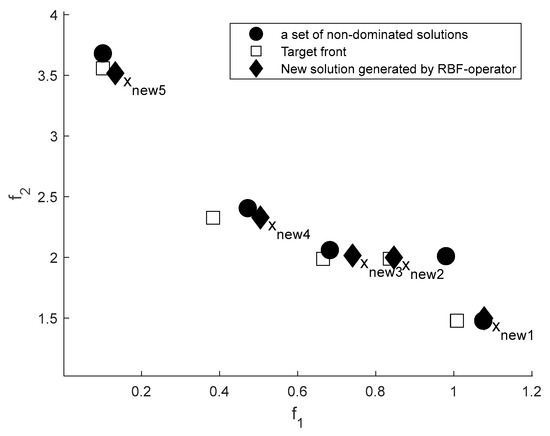
Figure 8. Plot of a set of non-dominated solutions, target points, and real function points obtained.

The proposed RBF-learning operator-assisted A-MRPBIL-DE is referred to as A-MRPBIL-DE-RBF. In the current study, a linear kernel function is employed in the RBF model. Specifically, ${\mathit{A}}_{ij}={\left\{K\left(\left|\left|\mathit{f}-{\overline{\mathit{f}}}^i\right|\right|\right)\right\}}_{N\times 1}={\left\{\left|\left|\mathit{f}-{\overline{\mathit{f}}}^i\right|\right|\right\}}_{N\times 1}$ based on Equation (14) and ${\mathit{A}}_{ij}=\left[K\left(\left|\left|{\mathbf{f}}^{\mathrm{i}}-{\mathbf{f}}^{\mathrm{j}}\right|\right|\right)\right]=\left[\left|{\mathit{f}}^i-{\mathit{f}}^j\right|\right]$ from Equation (16). This approach is applied to predict solutions (generate heuristic solutions in a metaheuristic algorithm) based on the target functions defined by Equation (17). The target function, or approximate Pareto front, is designed to be close to, but more advanced than, a set of non-dominated solutions. A linear RBF approximation is sufficiently accurate and requires less computation effort.

The main search procedure is similar to A-MRPBIL-DE, comprising an initialization process, RPBIL reproduction process, DE reproduction process, Pareto selection, and processing parameter adaptation. However, for the A-MRPBIL-DE-RBF, an RBF-learning operator is applied to generate several solutions after finishing the DE reproduction process. Then, Pareto selection is performed. This process is employed to enhance both search exploitation, based on the advantageous target points predefined, and exploration, which can be improved due to the uncertainty of the RBF model. The main search procedure of the A-MRPBIL-DE-RBF is shown in Algorithm 2.

Algorithm 2 A-MRPBIL-DE-RBF

Input: Number of iterations (NG), population size (NP), number of design domain subintervals (nI), number of trays (NT), Pareto archive size (NA), population size of the RBF operation (NRBF). Output: A Main Procedure Initialization 1: Define Pij = nI/Np for each tray, a Pareto archive A = {}. 2: Generate a real-coded population X from the probability trays and evaluate objective function values. 3: Select non-dominated solutions from X∪A and save them to A. 4: Set initial PMum = 0.5, Pxrm = 0.5, Fm = 0.5, CRm = 0.5. 5: Set initial goodPMum = {}, goodPxrm = {}, goodCR = {} and goodF = {}. 6: nFEs = 0 and maxFEs = NG × NP. 7: While nFEs < maxFE. Update population using RPBIL operation 8: Divide the non-dominated solutions into NT groups using a clustering technique and find the centroid rG of each group. 9: Update the probability trays using rG. 10: Generate a real-code population X from the probability trays. Update population using a DE operation 11: For j = 1 to NP.  11.1: Generate PMu, Pxr, and CR by normal random distribution and generate F using   the Lehmer mean technique.  11.2: Randomly select a solution xbest from the Pareto archive A.  11.3: Randomly select four solutions, xr1, xr2, xr3, and xr4.   11.3.1 If rand < Pxr, select the xr1, xr2, xr3, and xr4 from the current population X.   11.3.2 Otherwise, select the xr1, xr2,xr3, and xr4 from Pareto archive A.  11.4: Generate a new solution using the mutation schemes in Equation (6).  11.5: Perform crossover schemes in Equation (7).  11.6: Save the newly generated solution in Y. 12: End. 13: Evaluate objective function values of the new population in Y. 14: nFEs = nFEs + NP. RBF-learning operation 15: Randomly select NRBF points in a set of non-dominated solutions. 16: For j = 1 to NRBF.  16.1: Compute the target point using Equation (17).  16.2: Apply Equation (14) to generate a new solution.  16.3: Save the newly generated solution in Z. 17: End. 18: Evaluate objective function values of the new population in Z. 19: nFEs = nFEs + NRBF. Pareto selection 20: Select non-dominated solutions from Z∪Y∪A and save them as A. For each yi∈Y that dominates at least one solution in A, the parameters, PMu, Pxr, CR, and F index i are saved to goodPMu, goodPxr, goodCR, and goodF, respectively. Processing parameter adaption 21: Update the parameters, PMum, Pxrm Fm, and CRm using Equations (8)–(11). 22: If the number of A is larger than NA, remove some of the members in A using a clustering technique. 23: End.

4. Numerical Experiments

To evaluate the performance of the proposed A-MRPBIL-DE-RBF, seven many-objective metaheuristics (MnMHs) are employed along with the proposed algorithm to solve the robust optimum fixed-structure heading autopilot flight controller design problem, as detailed in Section 2, the benchmark test suite shown in Table 1, and the real-world test problems, as detailed in Table 2.

Table 1. Characteristics of many-objective optimization benchmark test suites [33].

Problem	Characteristics	Obj	Problem	Characteristics	Obj
MaF1	Linear	3	DTLZ2	Concave	4
MaF2	Concave	3	DTLZ4	Concave, Biased	4
MaF5	Convex, Biased	3	DTLZ5	Degenerate	4
MaF6	Concave, Degenerate	3	DTLZ6	Biased, Degenerate	4
MaF7	Mixed, Disconnected, Multimodal	3
MaF8	Linear, Degenerate	10	WFG2	Convex, disconnected, multi-modal, non-separable	5
MaF9	Linear, Degenerate	10
MaF10	Mixed, biased	3	WFG4	Concave, multi-modal	5
MaF11	Convex, disconnected, nonseparable	3
MaF12	Concave, Non-separable, Biased deceptive	3	WFG7	Concave, biased	5
MaF13	Concave, Unimodal, Non-separable, Degenerate	3	WFG8	Concave, biased, non-separable	5
MaF14	Linear, partially separable, large-scale	3	WFG9	Concave, biased, multi-modal, deceptive, non-separable	5
MaF15	Convex, partially separable, large scale	3

Table 2. Properties of the 9 test problems [34]. M and D denote the number of objectives and the number of decision variables, respectively. The type of design variables, the shape of the Pareto front, and other information are also described.

Problem	Original Name	M	D	Variables	Pareto Front
RE2-4-1	Four-bar truss design	2	4	Continuous	Convex
RE2-3-2	Reinforced concrete beam design	2	3	Mixed	Mixed
RE3-3-1	Two-bar truss design	3	3	Continuous	Unknown
RE3-4-2	Welded beam design	3	4	Continuous	Unknown
RE3-5-4	Vehicle crashworthiness design	3	5	Continuous	Unknown
RE3-7-5	Speed reducer design	3	7	Mixed	Unknown
RE3-4-7	Rocket injector design	3	4	Continuous	Unknown
RE4-7-1	Car side impact design	4	7	Continuous	Unknown
RE4-6-2	Conceptual marine design	4	6	Continuous	Unknown

The MnMHs used in this study are as follows:

• A knee point-driven evolutionary algorithm for many-objective optimization (MnKnEA) [35];
• A reference vector-guided evolutionary algorithm for many-objective optimization (RVEA) [36];
• Multi-objective Grey Wolf Optimizer: a novel algorithm for multi-criterion optimization (MOGWO) [37];
• An evolutionary many-objective optimization algorithm using reference-point-based non-dominated sorting (NSGA-III) [38];
• Success history-based adaptive multi-objective differential evolution (SHAMODE) [39];
• Hybrid real-code population-based incremental learning and differential evolution algorithm (MRPBIL-DE) [29];
• Hybrid real code population-based incremental learning and differential evolutionary algorithm with adaptive parameters (A-MRPBIL-DE) [27];
• A-MRPBIL-DE-RBF (Algorithm 2).

Each optimizer is employed to solve the robust optimum fixed-structure heading autopilot flight controller design problem and the benchmark test suites for 30 optimization runs. The maximum number of iterations and population size are both set at 100, while the maximum number of Pareto optimal solutions is 500. In cases where any MnMH performs a different number of iterations and population size, they are terminated at the same number of function evaluations, 100 × 100 evaluations.

Performance assessment is conducted using hypervolume (HV), generational distance (GD), inverted generational distance (IGD), and spacing-to-extent (STE). The Friedman test is employed for significance ranking with a 95% confidence level. The hypervolume represents the advancement of the Pareto front based on the reference points, while spacing-to-extent denotes the ratio of spacing to the extent of the Pareto front. The generational distance provides the degree of proximity based on the distance between the Pareto front and a subset of the true Pareto front, while the inverted generational distance determines the average distance from a Pareto front relative to a reference set. The four metrics are tested to measure different aspects of algorithm performance, where lower GD, IGD, and STE values, and higher HV indicate a better Pareto front.

5. Results and Discussion

5.1. Robust Optimum Fixed-Structure Heading Autopilot Flight Controller Design Problem

After conducting 30 optimization runs for all MnMHs to solve the proposed robust optimum fixed-structure heading autopilot flight controller design problem, MnMH performance was evaluated. Hypervolume (HV), spacing-to-extent (STE), generational distance (GD), and inverted generational distance (IGD) were used as indicators. The statistical results of HV, STE, GD, and IGD are presented in Table 3. The subscripts AV, best, worst, SD, and Frank denote the average, the best, the worst, standard deviation, and Friedman’s ranking score, respectively, obtained from 30 optimization runs for each algorithm. The mean values of each indicator were used to assess the MnMHs’ search convergence speed, while the number of successful runs was employed to measure MnMHs’ search consistency. In cases where the algorithms achieve the same number of successful runs, standard deviation (SD) values are considered. Better results are indicated by higher HV and lower STE, GD, and IGD values.

Table 3. Statistical results of hypervolume (HV), spacing-to-extent (STE), generational distance (GD), and inverted generational distance (IGD) (Bold indicates the best value).

Algorithm	MnKnEA	RVEA	MOGWO	NSGA_III	SHAMODE	MRPBIL-DE	A-MRPBIL-DE	A-MRPBIL-DE-RBF
No. of success full run	27	0	14	0	1	30	30	30
${\mathrm{H}\mathrm{V}}_{\mathrm{A}\mathrm{V}}$	4.253 × 10−1	NA	1.583 × 10−1	NA	1.791 × 10−2	4.051 × 10−1	5.201 × 10−1	5.284 × 10−1
${\mathrm{H}\mathrm{V}}_{\mathrm{b}\mathrm{e}\mathrm{s}\mathrm{t}}$	5.217 × 10−1	NA	5.208 × 10−1	NA	5.374 × 10−1	5.028 × 10−1	5.368 × 10−1	5.453 × 10−1
${\mathrm{H}\mathrm{V}}_{\mathrm{w}\mathrm{o}\mathrm{r}\mathrm{s}\mathrm{t}}$	0.000	NA	0.000	NA	0.000	1.589 × 10−3	4.662 × 10−1	5.142 × 10−1
${\mathrm{H}\mathrm{V}}_{\mathrm{S}\mathrm{D}}$	1.506 × 10−1	NA	2.080 × 10−1	NA	9.812 × 10−2	1.188 × 10−1	1.305 × 10−2	9.207 × 10−3
${\mathrm{H}\mathrm{V}}_{\mathrm{F}\mathrm{r}\mathrm{a}\mathrm{n}\mathrm{k}}$	3.62	6.70	5.32	6.70	6.53	3.97	1.83	1.33
${\mathrm{S}\mathrm{T}\mathrm{E}}_{\mathrm{A}\mathrm{V}}$	1.000 × 109	NA	5.333 × 109	NA	9.667 × 109	6.667 × 1018	6.958 × 10−3	4.075 × 10−3
${\mathrm{S}\mathrm{T}\mathrm{E}}_{\mathrm{b}\mathrm{e}\mathrm{s}\mathrm{t}}$	NA	NA	NA	NA	NA	8.699 × 10−3	4.308 × 10−3	2.580 × 10−3
${\mathrm{S}\mathrm{T}\mathrm{E}}_{\mathrm{w}\mathrm{o}\mathrm{r}\mathrm{s}\mathrm{t}}$	1.000 × 100	NA	1.000 × 100	NA	1.000 × 100	1.000 × 1020	1.560 × 10−2	8.051 × 10−3
${\mathrm{S}\mathrm{T}\mathrm{E}}_{\mathrm{S}\mathrm{D}}$	3.051 × 109	NA	5.074 × 109	NA	1.826 × 109	2.537 × 1019	2.651 × 10−3	1.143 × 10−3
${\mathrm{S}\mathrm{T}\mathrm{E}}_{\mathrm{F}\mathrm{r}\mathrm{a}\mathrm{n}\mathrm{k}}$	4.35	6.63	4.18	6.63	6.50	4.03	2.40	1.27
${\mathrm{G}\mathrm{D}}_{\mathrm{A}\mathrm{V}}$	2.597 × 101	NA	1.344 × 102	NA	2.423 × 102	3.316	1.559 × 10−1	1.449 × 10−1
${\mathrm{G}\mathrm{D}}_{\mathrm{b}\mathrm{e}\mathrm{s}\mathrm{t}}$	NA	NA	NA	NA	NA	2.489 × 10−1	7.448 × 10−2	7.467 × 10−2
${\mathrm{G}\mathrm{D}}_{\mathrm{w}\mathrm{o}\mathrm{r}\mathrm{s}\mathrm{t}}$	2.506 × 102	NA	2.506 × 102	NA	2.506 × 102	4.599 × 101	6.063 × 10−1	3.997 × 10−1
${\mathrm{G}\mathrm{D}}_{\mathrm{S}\mathrm{D}}$	7.618 × 101	NA	1.264 × 102	NA	4.573 × 101	8.490	1.081 × 10−1	5.984 × 10−2
${\mathrm{G}\mathrm{D}}_{\mathrm{F}\mathrm{r}\mathrm{a}\mathrm{n}\mathrm{k}}$	3.95	6.70	4.75	6.70	6.53	4.00	1.60	1.77
${\mathrm{I}\mathrm{G}\mathrm{D}}_{\mathrm{A}\mathrm{V}}$	7.038 × 101	NA	3.146 × 102	NA	5.047 × 102	3.336 × 101	1.178 × 101	4.831
${\mathrm{I}\mathrm{G}\mathrm{D}}_{\mathrm{b}\mathrm{e}\mathrm{s}\mathrm{t}}$	NA	NA	NA	NA	NA	9.531	4.578	1.991
${\mathrm{I}\mathrm{G}\mathrm{D}}_{\mathrm{w}\mathrm{o}\mathrm{r}\mathrm{s}\mathrm{t}}$	5.218 × 102	NA	5.218 × 102	NA	5.218 × 102	2.736 × 102	2.665 × 101	1.020 × 101
${\mathrm{I}\mathrm{G}\mathrm{D}}_{\mathrm{S}\mathrm{D}}$	1.535 × 102	NA	2.339 × 102	NA	9.407 × 101	4.981 × 101	5.333	2.030
${\mathrm{I}\mathrm{G}\mathrm{D}}_{\mathrm{F}\mathrm{r}\mathrm{a}\mathrm{n}\mathrm{k}}$	3.48	6.70	5.02	6.70	6.53	3.90	2.50	1.17
${\mathrm{S}\mathrm{U}\mathrm{M}}_{\mathrm{F}\mathrm{r}\mathrm{a}\mathrm{n}\mathrm{k}}$	15.40	26.73	19.27	26.73	26.10	15.90	8.33	5.53

In assessing search convergence based on the mean values of all indicators, the best performer across all indicators is the proposed A-MRPBIL-DE-RBF algorithm, with A-MRPBIL-DE as the second-best. MnKnEA and MOGWO ranked third based on HV and STE, while MRPBIL-DE ranked third based on GD and IGD. The top performers are A-MRPBIL-DE-RBF, A-MRPBIL-DE, and MRPBIL-DE, each achieving 30 out of 30 successful runs when evaluated for search consistency. However, when considering the standard deviation (SD) values for these top three algorithms, A-MRPBIL-DE-RBF is the most consistent across each indicator.

The overall search performance based on Friedman’s ranking score indicates that the best performer across all indicators, except for the GD indicator, is the proposed A-MRPBIL-DE-RBF, while A-MRPBIL-DE is the best performer based on Friedman’s ranking score for the GD indicator. A summary of Friedman’s ranking score for each indicator shows that the best performer is A-MRPBIL-DE-RBF. The second and third best performers are, respectively, A-MRPBIL-DE and MRPBIL-DE.

Figure 9 depicts a convergence plot of all algorithms based on the average HV values from 30 optimization runs for solving the proposed robust optimum fixed-structure heading autopilot flight controller design problem. The figure illustrates that A-MRPBIL-DE-RBF and A-MRPBIL-DE algorithms are the best performing, achieving the most advanced Pareto front from the beginning of the search process. Notably, A-MRPBIL-DE-RBF emerges as the most advanced algorithm as the search progresses, particularly after approximately 1500 function evaluations. Initially, MRPBIL-DE appears to be the third-best performer, but after around 6500 function evaluations, MnKnEA outperforms the MRPBIL-DE algorithm.

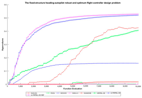
Figure 9. Average hypervolume versus function evaluation.

While SHAMODE, NSGA-III, and RVEA may seem to struggle with the proposed many-objective optimization problems, it is not implied that these algorithms are inherently inferior. As stated in the “no free lunch theorem” [34], no metaheuristic is universally superior across all problems.

Figure 10 presents the parallel coordinates plot of the final Pareto fronts from the best runs of A-MRPBIL-DE and A-MRPBIL-DE-RBF. The dashed line illustrates an example of a Pareto point where objective function 4 is minimized. When comparing Pareto points from both methods that achieve a similarly minimized objective function 4, the proposed A-MRPBIL-DE-RBF yields lower values for the other objective functions than A-MRPBIL-DE. This indicates that the proposed method achieves a more advanced Pareto front. Additionally, the distribution of lines in the figure suggests that A-MRPBIL-DE-RBF provides a more diverse and well-distributed set of solutions.

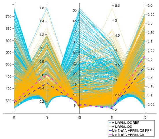
Figure 10. Parallel coordinates plot of the final Pareto front from the best run of A-MRPBIL-DE compared with A-MRPBIL-DE-RBF.

In summary, the findings suggest that the proposed A-MRPBIL-DE-RBF is the best performer for solving the robust optimum fixed-structure heading autopilot flight controller design problem. The integration of an RBF-learning operator into the original A-MRPBIL-DE has been successful, leading to an improvement in its search performance for such a multi-objective optimization problem.

Figure 11 displays the step responses with ±40% uncertainty of a step $\psi$ input for the selected Pareto solution with minimum f₁, f₂, f_3, and f₄ from the best run of the proposed A-MRPBIL-DE-RBF. Table 4 shows their objective and constraint function values. From Figure 11, all controllers that aimed to minimize all objective functions remained stable, with variations in response representing trade-offs between objective function values. The solution that minimizes f₁ shows fast and accurate tracking of the reference but exhibits low stability or high peak response. However, the system that minimizes f₂ demonstrates the highest stability and requires fewer control surface deflections. Table 4 indicates that all control systems selected from the Pareto solution satisfy all constraint requirements. Based on this study, within a single run, different robust and optimum heading autopilot systems with various performance levels satisfy all system requirements. All can be used for decision-making.

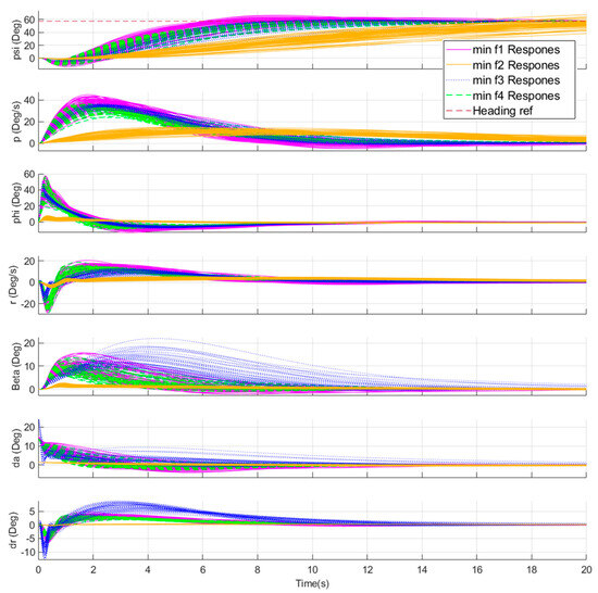
Figure 11. Step responses from the best solutions on the Pareto front min f₁, f₂, f_3, and f₄ with ±40% uncertainty of non-dimensional derivatives.

Table 4. Optimum controller and performance of the control system obtained from the best run of A-MRPBIL-DE-RBF (Bold indicates the best value).

Pareto Solution Selected by	Min f1	Min f2	Min f3	Min f4
$f_1\left(\mathit{x}\right)$	315.2015	729.1170	396.5011	340.7324
$f_2\left(\mathit{x}\right)$	0.4467	0.0919	1.1877	0.4720
$f_3\left(\mathit{x}\right)$	6.2251	50.9858	3.4840	5.6052
$f_4\left(\mathit{x}\right)$	2.3645	4.1442	2.6797	2.0324
$K_{\psi }$	2.0938	1.4033	0.9760	2.4914
$K_{\varphi }$	${\displaystyle \frac{0.1241s+0}{s}}$	${\displaystyle \frac{0.0169s+0}{s}}$	${\displaystyle \frac{0.4475s+0}{s}}$	${\displaystyle \frac{0.0960s+0}{s}}$
$K_p$	0.2885	0.0831	0.5693	0.3473
$K_r$	0.2293	0.0639	0.6673	0.2188
$\max ({\lambda }_A)<0$	−0.3960	−0.1318	−0.3705	−0.3892
$\mathit{settling} \mathit{time}\le 30 s$	11.3530	22.7483	10.9241	12.1884
$\%overshoot\le 5\%$	3.1304	1.5563	0.5402	0.0000
$\mathit{rise} \mathit{time}\le 15 sec$	3.8959	14.5004	6.1637	6.3304
$\%\left|\left.{\psi }_{t_{\infty }}-{\psi }_{ref}\right|\right.\le 2\%$	4.86 × 10−7	1.38 × 10−1	2.38 × 10−6	9.14 × 10−7
$\beta \le 20 deg$	9.5330	1.6137	12.1274	8.5390
$p\le 40 deg/s$	38.9385	11.5967	34.4850	32.3438
$\varphi \le 40 deg$	38.0397	4.4873	39.2341	36.6120
$r\le 20 deg/s$	19.9711	4.1466	12.8181	19.5356
${\delta }_a\le 30 deg$	14.8937	1.3563	25.0230	13.7105
${\delta }_r\le 30 deg$	4.5793	0.2650	8.5531	4.2740

5.2. The Benchmark Test Suites

This paper focuses on evaluating the performance of the proposed A-MRPBIL-DE-RBF for a specific many-objective optimization problem in the design of a heading-ahead autonomous navigation system. It also examines its effectiveness using additional benchmark test suites to ensure applicability to other problems.

After conducting 30 optimization runs for each MnMH on the benchmark test suites, their performance was assessed using the HV, STE, GD, and IGD performance indicators. Additionally, Friedman’s rank test was performed to statistically rank the various algorithms. The mean or overall Friedman rank is derived from the average rankings based on HV, STE, GD, and IGD.

Table 5 presents the Friedman ranks from HV, STE, GD, IGD, and mean values of the Friedman ranks of all optimizers on the benchmark test suites. The experimental results demonstrate the efficiency of the algorithms in solving each problem. Furthermore, the Friedman rank of A-MRPBIL-DE-RBF is significantly higher than that of the original A-MRPBIL-DE before improvement, considering the HV, STE, GD, and IGD indicators.

Table 5. Friedman’s ranks from HV, STE, GD, IGD, and mean values of these ranks of all optimizers on the benchmark test suites (Bold indicates the best value).

Problems		MaF1	MaF2	MaF5	MaF6	MaF7	MaF8	MaF9	MaF10	MaF11	MaF12	MaF13	MaF14	MaF15	DTLZ2	DTLZ4	DTLZ5	DTLZ6	WFG2	WFG4	WFG7	WFG8	WFG9
Algorithm
MnKnEA	${\mathrm{H}\mathrm{V}}_{\mathrm{F}\mathrm{r}\mathrm{a}\mathrm{n}\mathrm{k}}$	2.83	2.00	4.47	4.00	2.00	4.70	5.17	1.00	1.00	2.67	5.20	5.52	6.07	3.00	1.93	3.23	3.07	1.00	1.00	1.17	1.27	1.07
	${\mathrm{S}\mathrm{T}\mathrm{E}}_{\mathrm{F}\mathrm{r}\mathrm{a}\mathrm{n}\mathrm{k}}$	6.90	6.70	6.10	4.00	6.00	5.27	4.03	3.30	7.77	6.90	6.57	3.90	6.60	7.53	7.13	6.03	5.90	7.10	7.30	7.60	7.97	6.17
	${\mathrm{G}\mathrm{D}}_{\mathrm{F}\mathrm{r}\mathrm{a}\mathrm{n}\mathrm{k}}$	5.27	6.63	4.63	3.70	5.27	4.50	7.73	1.00	6.00	6.03	4.60	2.93	4.10	4.10	3.90	7.83	3.77	7.00	7.00	7.00	5.80	6.93
	${\mathrm{I}\mathrm{G}\mathrm{D}}_{\mathrm{F}\mathrm{r}\mathrm{a}\mathrm{n}\mathrm{k}}$	4.57	4.50	5.17	4.00	2.50	4.50	7.33	1.00	5.37	4.00	6.23	4.13	5.63	2.33	2.50	5.93	2.20	2.40	3.07	2.07	1.20	1.47
	${\mathrm{M}\mathrm{e}\mathrm{a}\mathrm{n}}_{\mathrm{F}\mathrm{r}\mathrm{a}\mathrm{n}\mathrm{k}}$	4.89	4.96	5.09	3.93	3.94	4.74	6.07	1.58	5.04	4.90	5.65	4.12	5.60	4.24	3.87	5.76	3.74	4.38	4.59	4.46	4.06	3.91
RVEA	${\mathrm{H}\mathrm{V}}_{\mathrm{F}\mathrm{r}\mathrm{a}\mathrm{n}\mathrm{k}}$	6.07	3.97	5.03	7.18	6.33	6.52	4.92	2.00	2.80	4.93	5.80	5.52	6.15	1.60	1.97	1.03	3.40	2.00	2.00	1.83	1.73	2.17
	${\mathrm{S}\mathrm{T}\mathrm{E}}_{\mathrm{F}\mathrm{r}\mathrm{a}\mathrm{n}\mathrm{k}}$	6.90	6.33	6.23	7.33	7.20	7.32	7.90	7.43	5.87	6.23	6.93	7.10	7.93	6.13	6.80	7.90	7.80	6.13	6.00	6.27	6.20	6.83
	${\mathrm{G}\mathrm{D}}_{\mathrm{F}\mathrm{r}\mathrm{a}\mathrm{n}\mathrm{k}}$	7.33	8.00	6.47	7.53	7.00	7.33	1.17	6.47	6.97	6.97	4.37	4.20	6.60	5.30	4.63	4.47	5.37	5.60	5.17	5.77	6.67	6.07
	${\mathrm{I}\mathrm{G}\mathrm{D}}_{\mathrm{F}\mathrm{r}\mathrm{a}\mathrm{n}\mathrm{k}}$	6.47	6.97	5.07	7.03	5.83	6.87	4.97	2.00	3.97	4.87	4.87	6.33	5.40	2.17	1.90	2.30	2.27	5.70	1.53	1.10	1.80	1.97
	${\mathrm{M}\mathrm{e}\mathrm{a}\mathrm{n}}_{\mathrm{F}\mathrm{r}\mathrm{a}\mathrm{n}\mathrm{k}}$	6.69	6.32	5.70	7.27	6.59	7.01	4.74	4.48	4.90	5.75	5.49	5.79	6.52	3.80	3.83	3.93	4.71	4.86	3.68	3.74	4.10	4.26
MOGWO	${\mathrm{H}\mathrm{V}}_{\mathrm{F}\mathrm{r}\mathrm{a}\mathrm{n}\mathrm{k}}$	3.80	3.97	6.47	5.63	5.83	6.57	5.17	6.93	3.37	2.00	7.60	5.38	2.10	4.90	6.07	3.63	1.77	3.13	7.73	7.00	7.80	7.10
	${\mathrm{S}\mathrm{T}\mathrm{E}}_{\mathrm{F}\mathrm{r}\mathrm{a}\mathrm{n}\mathrm{k}}$	4.90	5.00	4.67	5.63	2.90	1.78	6.97	6.03	3.63	5.00	5.73	5.53	4.53	4.63	1.53	4.90	5.33	4.87	5.00	5.00	5.00	5.03
	${\mathrm{G}\mathrm{D}}_{\mathrm{F}\mathrm{r}\mathrm{a}\mathrm{n}\mathrm{k}}$	2.17	1.30	6.37	5.90	1.07	5.90	5.87	7.00	1.93	1.50	7.97	5.43	1.33	2.17	5.13	1.77	6.57	1.10	5.53	4.00	5.53	4.47
	${\mathrm{I}\mathrm{G}\mathrm{D}}_{\mathrm{F}\mathrm{r}\mathrm{a}\mathrm{n}\mathrm{k}}$	3.33	2.37	6.47	5.93	6.40	6.73	7.07	6.77	3.10	2.53	6.93	4.70	2.00	5.17	6.27	2.20	1.83	4.17	7.07	7.00	7.30	7.17
	${\mathrm{M}\mathrm{e}\mathrm{a}\mathrm{n}}_{\mathrm{F}\mathrm{r}\mathrm{a}\mathrm{n}\mathrm{k}}$	3.55	3.16	6.00	5.77	4.05	5.25	6.27	6.68	3.01	2.76	7.06	5.26	2.49	4.22	4.75	3.13	3.88	3.32	6.33	5.75	6.41	5.94
NSGA_III	${\mathrm{H}\mathrm{V}}_{\mathrm{F}\mathrm{r}\mathrm{a}\mathrm{n}\mathrm{k}}$	7.73	8.00	7.73	7.72	8.00	5.93	4.05	7.97	7.70	8.00	7.00	5.52	6.15	8.00	7.80	8.00	5.75	7.63	7.27	8.00	7.20	7.90
	${\mathrm{S}\mathrm{T}\mathrm{E}}_{\mathrm{F}\mathrm{r}\mathrm{a}\mathrm{n}\mathrm{k}}$	7.20	7.97	7.47	7.20	7.80	6.97	5.10	6.43	7.20	7.87	5.60	2.57	2.93	7.33	6.10	7.07	6.77	7.70	7.70	7.13	6.83	7.97
	${\mathrm{G}\mathrm{D}}_{\mathrm{F}\mathrm{r}\mathrm{a}\mathrm{n}\mathrm{k}}$	7.67	6.37	6.73	7.37	8.00	6.33	6.43	6.93	8.00	8.00	1.87	7.73	7.97	8.00	7.63	6.83	8.00	8.00	8.00	8.00	8.00	8.00
	${\mathrm{I}\mathrm{G}\mathrm{D}}_{\mathrm{F}\mathrm{r}\mathrm{a}\mathrm{n}\mathrm{k}}$	7.67	7.97	7.70	7.83	8.00	5.80	3.97	8.00	7.93	8.00	7.63	8.00	7.97	8.00	7.77	8.00	7.93	8.00	7.93	8.00	7.70	7.83
	${\mathrm{M}\mathrm{e}\mathrm{a}\mathrm{n}}_{\mathrm{F}\mathrm{r}\mathrm{a}\mathrm{n}\mathrm{k}}$	7.57	7.58	7.41	7.53	7.95	6.26	4.89	7.33	7.71	7.97	5.53	5.96	6.26	7.83	7.33	7.48	7.11	7.83	7.73	7.78	7.43	7.93
SHAMODE	${\mathrm{H}\mathrm{V}}_{\mathrm{F}\mathrm{r}\mathrm{a}\mathrm{n}\mathrm{k}}$	2.60	4.63	3.40	1.00	4.00	1.67	5.17	3.00	3.87	3.37	2.07	5.52	1.57	6.40	6.17	4.73	5.75	4.97	4.30	4.03	4.17	4.20
	${\mathrm{S}\mathrm{T}\mathrm{E}}_{\mathrm{F}\mathrm{r}\mathrm{a}\mathrm{n}\mathrm{k}}$	1.90	1.53	2.80	1.00	2.63	2.40	2.90	1.50	4.10	1.93	3.23	5.43	6.20	1.53	3.60	3.10	2.13	3.67	1.20	1.17	1.17	1.80
	${\mathrm{G}\mathrm{D}}_{\mathrm{F}\mathrm{r}\mathrm{a}\mathrm{n}\mathrm{k}}$	2.77	2.90	2.93	1.00	4.97	3.00	5.37	2.43	2.53	2.43	2.97	5.63	2.03	7.00	6.27	1.57	5.10	4.00	2.20	2.00	2.27	2.13
	${\mathrm{I}\mathrm{G}\mathrm{D}}_{\mathrm{F}\mathrm{r}\mathrm{a}\mathrm{n}\mathrm{k}}$	2.17	3.00	2.97	1.00	3.23	1.40	4.50	3.00	1.50	2.23	1.60	6.47	1.47	6.37	5.83	4.03	7.07	2.67	5.43	5.10	5.73	4.13
	${\mathrm{M}\mathrm{e}\mathrm{a}\mathrm{n}}_{\mathrm{F}\mathrm{r}\mathrm{a}\mathrm{n}\mathrm{k}}$	2.36	3.02	3.03	1.00	3.71	2.12	4.49	2.48	3.00	2.49	2.47	5.76	2.82	5.33	5.47	3.36	5.01	3.83	3.28	3.08	3.34	3.07
MRPBIL-DE	${\mathrm{H}\mathrm{V}}_{\mathrm{F}\mathrm{r}\mathrm{a}\mathrm{n}\mathrm{k}}$	7.20	7.00	5.60	5.47	3.57	6.28	3.78	5.93	7.23	6.57	4.17	5.03	2.33	6.50	5.80	6.67	5.75	6.87	5.87	5.67	5.30	5.97
	${\mathrm{S}\mathrm{T}\mathrm{E}}_{\mathrm{F}\mathrm{r}\mathrm{a}\mathrm{n}\mathrm{k}}$	4.07	4.00	3.50	5.83	2.77	4.47	2.73	3.47	1.93	3.40	2.77	6.37	4.33	4.37	3.27	3.60	4.00	2.00	1.90	3.13	3.23	2.83
	${\mathrm{G}\mathrm{D}}_{\mathrm{F}\mathrm{r}\mathrm{a}\mathrm{n}\mathrm{k}}$	5.73	4.47	4.93	5.20	3.00	5.63	2.90	4.27	4.50	4.67	5.47	6.93	2.67	5.40	5.37	3.37	3.97	4.43	3.80	3.87	2.83	4.33
	${\mathrm{I}\mathrm{G}\mathrm{D}}_{\mathrm{F}\mathrm{r}\mathrm{a}\mathrm{n}\mathrm{k}}$	6.87	5.77	5.17	5.17	3.93	6.10	2.63	6.07	6.90	6.67	4.23	2.95	2.53	6.43	5.37	6.30	5.90	5.93	5.53	5.40	4.97	5.90
	${\mathrm{M}\mathrm{e}\mathrm{a}\mathrm{n}}_{\mathrm{F}\mathrm{r}\mathrm{a}\mathrm{n}\mathrm{k}}$	5.97	5.31	4.80	5.42	3.32	5.62	3.01	4.94	5.14	5.33	4.16	5.32	2.97	5.68	4.95	4.99	4.91	4.81	4.28	4.52	4.08	4.76
A-MRPBIL-DE	${\mathrm{H}\mathrm{V}}_{\mathrm{F}\mathrm{r}\mathrm{a}\mathrm{n}\mathrm{k}}$	4.77	5.43	2.20	2.63	4.97	2.43	3.40	4.50	6.03	6.17	2.23	1.52	6.07	4.20	3.63	6.17	5.45	6.47	4.83	5.30	5.50	4.83
	${\mathrm{S}\mathrm{T}\mathrm{E}}_{\mathrm{F}\mathrm{r}\mathrm{a}\mathrm{n}\mathrm{k}}$	2.90	2.97	2.83	2.63	4.07	4.00	2.93	3.47	3.87	2.27	3.00	2.67	1.97	2.90	4.33	2.27	2.10	2.87	3.73	3.40	2.90	2.60
	${\mathrm{G}\mathrm{D}}_{\mathrm{F}\mathrm{r}\mathrm{a}\mathrm{n}\mathrm{k}}$	4.00	4.53	2.37	2.53	4.50	1.67	3.40	3.53	4.23	4.23	3.90	1.77	5.77	3.03	1.77	5.33	1.43	3.97	3.27	4.33	3.87	3.07
	${\mathrm{I}\mathrm{G}\mathrm{D}}_{\mathrm{F}\mathrm{r}\mathrm{a}\mathrm{n}\mathrm{k}}$	3.93	4.40	2.17	2.60	4.73	2.47	2.67	4.43	5.43	5.93	2.10	1.57	6.60	4.03	3.50	5.67	4.47	5.83	3.70	4.50	4.27	4.97
	${\mathrm{M}\mathrm{e}\mathrm{a}\mathrm{n}}_{\mathrm{F}\mathrm{r}\mathrm{a}\mathrm{n}\mathrm{k}}$	3.90	4.33	2.39	2.60	4.57	2.64	3.10	3.98	4.89	4.65	2.81	1.88	5.10	3.54	3.31	4.86	3.36	4.79	3.88	4.38	4.14	3.87
A-MRPBIL-DE-RBF	${\mathrm{H}\mathrm{V}}_{\mathrm{F}\mathrm{r}\mathrm{a}\mathrm{n}\mathrm{k}}$	1.00	1.00	1.10	2.37	1.30	1.90	4.35	4.67	4.00	2.30	1.93	2.00	5.57	1.40	2.63	2.53	5.07	3.93	3.00	3.00	3.03	2.77
	${\mathrm{S}\mathrm{T}\mathrm{E}}_{\mathrm{F}\mathrm{r}\mathrm{a}\mathrm{n}\mathrm{k}}$	1.23	1.50	2.40	2.37	2.63	3.80	3.43	4.37	1.63	2.40	2.17	2.43	1.50	1.57	3.23	1.13	1.97	1.67	3.17	2.30	2.70	2.77
	${\mathrm{G}\mathrm{D}}_{\mathrm{F}\mathrm{r}\mathrm{a}\mathrm{n}\mathrm{k}}$	1.07	1.80	1.57	2.77	2.20	1.63	3.13	4.37	1.83	2.17	4.87	1.37	5.53	1.00	1.30	4.83	1.80	1.90	1.03	1.03	1.03	1.00
	${\mathrm{I}\mathrm{G}\mathrm{D}}_{\mathrm{F}\mathrm{r}\mathrm{a}\mathrm{n}\mathrm{k}}$	1.00	1.03	1.30	2.43	1.37	2.13	2.87	4.73	1.80	1.77	2.40	1.85	4.40	1.50	2.87	1.57	4.33	1.30	1.73	2.83	3.03	2.57
	${\mathrm{M}\mathrm{e}\mathrm{a}\mathrm{n}}_{\mathrm{F}\mathrm{r}\mathrm{a}\mathrm{n}\mathrm{k}}$	1.08	1.33	1.59	2.49	1.88	2.37	3.45	4.54	2.32	2.16	2.84	1.91	4.25	1.37	2.51	2.52	3.29	2.20	2.23	2.29	2.45	2.28

Table 6 presents the overall Friedman rank for the eight algorithms. The results clearly indicate that A-MRPBIL-DE-RBF achieves the highest ranking, with a total Friedman rank of 53.32, making it the best-performing algorithm for MaF1, MaF2, MaF5, MaF7, MaF11, MaF12, DTLZ2, DTLZ4, DTLZ5, DTLZ6, WFG2, WFG4, WFG7, WFG8, and WFG9. SHAMODE is the second best with an overall sum of Friedman’s rank of 74.48 but performs best for MaF6, MaF8, and MaF13. A-MRPBIL-DE secures third place with an overall Friedman rank of 82.97 and is the best performer for MaF14. MnKnEA, MRPBIL-DE, and MOGWO are the best performers for MaF10, MaF9, and MaF15, respectively. Performance details of the algorithms for each indicator are shown in Appendix A.

Table 6. Overall ranking based on mean values of the Friedman’s ranks of all optimizers on the benchmark test suites (Bold indicates the best value).

Problems	MnKnEA	RVEA	MOGWO	NSGA_III	SHAMODE	MRPBIL-DE	A-MRPBIL-DE	A-MRPBIL-DE-RBF
MaF1	4.89	6.69	3.55	7.57	2.36	5.97	3.90	1.08
MaF2	4.96	6.32	3.16	7.58	3.02	5.31	4.33	1.33
MaF5	5.09	5.70	5.99	7.41	3.03	4.80	2.39	1.59
MaF6	3.93	7.27	5.78	7.53	1.00	5.42	2.60	2.48
MaF7	3.94	6.59	4.05	7.95	3.71	3.32	4.57	1.88
MaF8	4.74	7.01	5.25	6.26	2.12	5.62	2.64	2.37
MaF9	6.07	4.74	6.27	4.89	4.48	3.01	3.10	3.45
MaF10	1.58	4.48	6.68	7.33	2.48	4.93	3.98	4.53
MaF11	5.03	4.90	3.01	7.71	3.00	5.14	4.89	2.32
MaF12	4.90	5.75	2.76	7.97	2.49	5.33	4.65	2.16
MaF13	5.65	5.49	7.06	5.53	2.47	4.16	2.81	2.84
MaF14	4.12	5.79	5.26	5.95	5.76	5.32	1.88	1.91
MaF15	5.60	6.52	2.49	6.25	2.82	2.97	5.10	4.25
DTLZ2	4.24	3.80	4.22	7.83	5.33	5.68	3.54	1.37
DTLZ4	3.87	3.83	4.75	7.33	5.47	4.95	3.31	2.51
DTLZ5	5.76	3.93	3.13	7.48	3.36	4.98	4.86	2.52
DTLZ6	3.73	4.71	3.88	7.11	5.01	4.90	3.36	3.29
WFG2	4.38	4.86	3.32	7.83	3.83	4.81	4.78	2.20
WFG4	4.59	3.68	6.33	7.73	3.28	4.28	3.88	2.23
WFG7	4.46	3.74	5.75	7.78	3.08	4.52	4.38	2.29
WFG8	4.06	4.10	6.41	7.43	3.33	4.08	4.13	2.45
WFG9	3.91	4.26	5.94	7.93	3.07	4.76	3.87	2.28
Sum ranks	99.49	114.13	105.02	158.36	74.48	104.24	82.97	53.32
Ranking	4	7	6	8	2	5	3	1

Figure 12 compares the Pareto fronts of the best runs of the proposed A-MRPBIL-DE-RBF and the original A-MRPBIL-DE for the benchmark functions, MaF1, MaF7, MaF11, and MaF15. The results indicate that A-MRPBIL-DE-RBF advances closer to the true fronts than the original A-MRPBIL-DE.

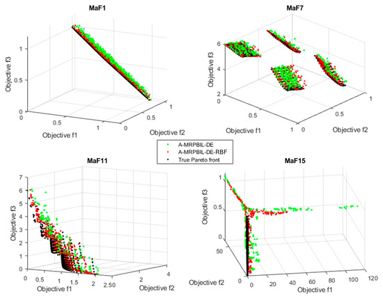
Figure 12. A Pareto front comparison of A-MRPBIL-DE, A-MRPBIL-DE-RBF, and true Pareto front.

5.3. The Real-World Test Problems

In addition to the benchmark test suite, real-world test problems (RE), as detailed in Table 2 [34], were also used to evaluate the proposed algorithm. Similarly to the benchmark test suite cases, each RE test problem was solved by each MnMH over 30 independent optimization runs. The number of iterations and the population size are both set at 100. The performance of the algorithms was assessed using four indicators: HV, STE, GD, and IGD. Additionally, Friedman’s rank test was applied to statistically rank the algorithms. The mean Friedman rank was computed as the average of rankings across all four performance metrics. The results are presented in Table 7, which clearly shows that the proposed A-MRPBIL-DE-RBF achieved the best overall performance across all RE test problems.

Table 7. Friedman’s ranks from HV, STE, GD, IGD, and mean values of these ranks of all optimizers on the RE test suites (Bold indicates the best value).

Problems Algorithm		RE2-4-1	RE2-3-2	RE3-3-1	RE3-4-2	RE3-5-4	RE3-7-5	RE3-4-7	RE4-7-1	RE4-6-2
MnKnEA	${\mathbf{H}\mathbf{V}}_{\mathbf{F}\mathbf{r}\mathbf{a}\mathbf{n}\mathbf{k}}$	7.53	7.30	7.87	7.63	7.93	8.00	7.20	6.47	7.83
	${\mathrm{S}\mathrm{T}\mathrm{E}}_{\mathrm{F}\mathrm{r}\mathrm{a}\mathrm{n}\mathrm{k}}$	7.93	7.10	7.20	7.87	8.00	7.97	7.60	7.97	7.47
	${\mathrm{G}\mathrm{D}}_{\mathrm{F}\mathrm{r}\mathrm{a}\mathrm{n}\mathrm{k}}$	8.00	7.83	1.27	3.23	8.00	7.93	8.00	7.90	7.97
	${\mathrm{I}\mathrm{G}\mathrm{D}}_{\mathrm{F}\mathrm{r}\mathrm{a}\mathrm{n}\mathrm{k}}$	7.23	7.37	7.87	6.93	7.43	6.00	7.10	6.50	7.53
	${\mathrm{M}\mathrm{e}\mathrm{a}\mathrm{n}}_{\mathrm{F}\mathrm{r}\mathrm{a}\mathrm{n}\mathrm{k}}$	7.68	7.40	6.05	6.42	7.84	7.48	7.48	7.21	7.70
RVEA	${\mathrm{H}\mathrm{V}}_{\mathrm{F}\mathrm{r}\mathrm{a}\mathrm{n}\mathrm{k}}$	7.47	6.87	4.13	7.30	6.50	6.00	6.17	6.63	7.17
	${\mathrm{S}\mathrm{T}\mathrm{E}}_{\mathrm{F}\mathrm{r}\mathrm{a}\mathrm{n}\mathrm{k}}$	6.97	7.27	6.80	6.97	6.67	6.90	6.20	6.90	7.37
	${\mathrm{G}\mathrm{D}}_{\mathrm{F}\mathrm{r}\mathrm{a}\mathrm{n}\mathrm{k}}$	6.30	5.83	2.73	1.27	6.13	1.67	7.00	6.43	6.93
	${\mathrm{I}\mathrm{G}\mathrm{D}}_{\mathrm{F}\mathrm{r}\mathrm{a}\mathrm{n}\mathrm{k}}$	7.60	6.77	6.67	7.83	7.03	7.93	6.00	7.10	6.00
	${\mathrm{M}\mathrm{e}\mathrm{a}\mathrm{n}}_{\mathrm{F}\mathrm{r}\mathrm{a}\mathrm{n}\mathrm{k}}$	7.08	6.68	5.08	5.84	6.58	5.63	6.34	6.77	6.87
MOGWO	${\mathrm{H}\mathrm{V}}_{\mathrm{F}\mathrm{r}\mathrm{a}\mathrm{n}\mathrm{k}}$	4.03	4.73	4.33	2.37	3.53	1.00	4.20	4.87	4.70
	${\mathrm{S}\mathrm{T}\mathrm{E}}_{\mathrm{F}\mathrm{r}\mathrm{a}\mathrm{n}\mathrm{k}}$	4.90	4.33	2.93	1.87	4.17	4.90	4.97	3.47	4.20
	${\mathrm{G}\mathrm{D}}_{\mathrm{F}\mathrm{r}\mathrm{a}\mathrm{n}\mathrm{k}}$	4.17	2.93	4.37	7.73	3.43	2.33	4.60	1.97	3.23
	${\mathrm{I}\mathrm{G}\mathrm{D}}_{\mathrm{F}\mathrm{r}\mathrm{a}\mathrm{n}\mathrm{k}}$	4.90	4.90	1.00	2.03	3.77	4.30	4.93	4.87	3.10
	${\mathrm{M}\mathrm{e}\mathrm{a}\mathrm{n}}_{\mathrm{F}\mathrm{r}\mathrm{a}\mathrm{n}\mathrm{k}}$	4.50	4.23	3.16	3.50	3.73	3.13	4.68	3.79	3.81
NSGA_III	${\mathrm{H}\mathrm{V}}_{\mathrm{F}\mathrm{r}\mathrm{a}\mathrm{n}\mathrm{k}}$	5.83	6.83	7.03	5.87	6.57	6.97	7.30	7.90	1.17
	${\mathrm{S}\mathrm{T}\mathrm{E}}_{\mathrm{F}\mathrm{r}\mathrm{a}\mathrm{n}\mathrm{k}}$	6.10	6.47	6.60	5.80	6.33	6.13	7.20	6.13	6.13
	${\mathrm{G}\mathrm{D}}_{\mathrm{F}\mathrm{r}\mathrm{a}\mathrm{n}\mathrm{k}}$	6.70	6.73	7.13	4.47	6.73	6.90	6.00	6.67	4.53
	${\mathrm{I}\mathrm{G}\mathrm{D}}_{\mathrm{F}\mathrm{r}\mathrm{a}\mathrm{n}\mathrm{k}}$	6.17	6.83	6.10	6.03	6.53	7.07	7.90	7.40	7.47
	${\mathrm{M}\mathrm{e}\mathrm{a}\mathrm{n}}_{\mathrm{F}\mathrm{r}\mathrm{a}\mathrm{n}\mathrm{k}}$	6.20	6.72	6.72	5.54	6.54	6.77	7.10	7.03	4.83
SHAMODE	${\mathrm{H}\mathrm{V}}_{\mathrm{F}\mathrm{r}\mathrm{a}\mathrm{n}\mathrm{k}}$	3.20	3.53	1.87	4.60	4.30	4.60	3.20	3.97	4.57
	${\mathrm{S}\mathrm{T}\mathrm{E}}_{\mathrm{F}\mathrm{r}\mathrm{a}\mathrm{n}\mathrm{k}}$	3.70	4.60	4.73	4.90	3.50	3.07	2.43	3.60	3.67
	${\mathrm{G}\mathrm{D}}_{\mathrm{F}\mathrm{r}\mathrm{a}\mathrm{n}\mathrm{k}}$	3.70	4.33	3.00	3.23	3.60	5.07	4.37	4.03	3.87
	${\mathrm{I}\mathrm{G}\mathrm{D}}_{\mathrm{F}\mathrm{r}\mathrm{a}\mathrm{n}\mathrm{k}}$	3.07	3.50	3.60	5.10	3.67	3.80	3.00	3.67	2.77
	${\mathrm{M}\mathrm{e}\mathrm{a}\mathrm{n}}_{\mathrm{F}\mathrm{r}\mathrm{a}\mathrm{n}\mathrm{k}}$	3.42	3.99	3.30	4.46	3.77	4.13	3.25	3.82	3.72
MRPBIL-DE	${\mathrm{H}\mathrm{V}}_{\mathrm{F}\mathrm{r}\mathrm{a}\mathrm{n}\mathrm{k}}$	4.87	3.60	3.87	1.83	2.87	2.83	4.27	3.17	5.10
	${\mathrm{S}\mathrm{T}\mathrm{E}}_{\mathrm{F}\mathrm{r}\mathrm{a}\mathrm{n}\mathrm{k}}$	3.30	2.67	1.93	3.10	2.70	1.90	4.03	3.23	2.27
	${\mathrm{G}\mathrm{D}}_{\mathrm{F}\mathrm{r}\mathrm{a}\mathrm{n}\mathrm{k}}$	2.73	3.20	6.90	5.53	3.13	3.63	1.27	2.73	3.40
	${\mathrm{I}\mathrm{G}\mathrm{D}}_{\mathrm{F}\mathrm{r}\mathrm{a}\mathrm{n}\mathrm{k}}$	4.03	3.60	4.87	2.97	3.10	2.93	4.07	3.43	5.00
	${\mathrm{M}\mathrm{e}\mathrm{a}\mathrm{n}}_{\mathrm{F}\mathrm{r}\mathrm{a}\mathrm{n}\mathrm{k}}$	3.73	3.27	4.39	3.36	2.95	2.83	3.41	3.14	3.94
A-MRPBIL-DE	${\mathrm{H}\mathrm{V}}_{\mathrm{F}\mathrm{r}\mathrm{a}\mathrm{n}\mathrm{k}}$	1.73	1.97	4.23	3.17	2.27	3.83	2.00	1.70	2.63
	${\mathrm{S}\mathrm{T}\mathrm{E}}_{\mathrm{F}\mathrm{r}\mathrm{a}\mathrm{n}\mathrm{k}}$	1.77	2.13	2.90	4.20	2.50	2.47	2.57	2.87	2.67
	${\mathrm{G}\mathrm{D}}_{\mathrm{F}\mathrm{r}\mathrm{a}\mathrm{n}\mathrm{k}}$	2.13	3.17	5.77	3.87	2.60	4.13	2.30	3.07	2.93
	${\mathrm{I}\mathrm{G}\mathrm{D}}_{\mathrm{F}\mathrm{r}\mathrm{a}\mathrm{n}\mathrm{k}}$	1.63	1.83	3.90	4.10	2.43	2.80	1.57	1.60	2.50
	${\mathrm{M}\mathrm{e}\mathrm{a}\mathrm{n}}_{\mathrm{F}\mathrm{r}\mathrm{a}\mathrm{n}\mathrm{k}}$	1.82	2.28	4.20	3.83	2.45	3.31	2.11	2.31	2.68
A-MRPBIL-DE-RBF	${\mathrm{H}\mathrm{V}}_{\mathrm{F}\mathrm{r}\mathrm{a}\mathrm{n}\mathrm{k}}$	1.33	1.17	2.67	3.23	2.03	2.77	1.67	1.30	2.83
	${\mathrm{S}\mathrm{T}\mathrm{E}}_{\mathrm{F}\mathrm{r}\mathrm{a}\mathrm{n}\mathrm{k}}$	1.33	1.43	2.90	1.30	2.13	2.67	1.00	1.83	2.23
	${\mathrm{G}\mathrm{D}}_{\mathrm{F}\mathrm{r}\mathrm{a}\mathrm{n}\mathrm{k}}$	2.27	1.97	4.83	6.67	2.37	4.33	2.47	3.20	3.13
	${\mathrm{I}\mathrm{G}\mathrm{D}}_{\mathrm{F}\mathrm{r}\mathrm{a}\mathrm{n}\mathrm{k}}$	1.37	1.20	2.00	1.00	2.03	1.17	1.43	1.43	1.63
	${\mathrm{M}\mathrm{e}\mathrm{a}\mathrm{n}}_{\mathrm{F}\mathrm{r}\mathrm{a}\mathrm{n}\mathrm{k}}$	1.58	1.44	3.10	3.05	2.14	2.73	1.64	1.94	2.46

Figure 13 shows the efficiency and effectiveness of the proposed RBF-learning operator. The percentage value determines the rate of the RBF-learning operator capable of producing non-dominated solutions at a particular iteration. If the value is 100%, that means all the design solutions generated by the RBF-learning operator are non-dominated on that iteration. The examination was made using the RE4-7-1 problem. The rate of producing non-dominated solutions by the original A-MRPBIL-DE operator is also given for comparison. As shown in the figure, the proposed learning operator consistently yields a higher rate of producing non-dominated solutions across the iterations. This confirms the effectiveness of the proposed RBF-learning operator in enhancing the performance of MnMHs.

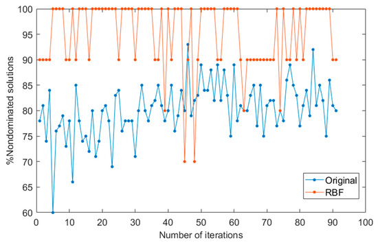
Figure 13. Comparison of the percentage of non-dominated solutions per iteration between the original reproduction operation and the proposed RBF learning-based reproduction operation.

Overall, A-MRPBIL-DE-RBF is the top performer in solving the benchmark test problems. Its performance is enhanced by integrating an RBF-learning operator into the original A-MRPBIL-DE, making it the best method for both the robust optimum fixed-structure heading autopilot flight controller design problem and the benchmark many-objective optimization test problems. However, as stated by the No Free Lunch Theorem, no single algorithm can perform best across all types of problems. Therefore, further investigation is needed for broader applications.

6. Conclusions

In this work, RBF-learning operator-assisted A-MRPBIL-DE is successfully presented for a robust optimum fixed-structure heading autopilot controller design. Several well-established MnMHs are used for comparison to identify the performance of the proposed algorithm. The robust optimum fixed-structure heading autopilot flight controller design, benchmark many-objective test problems, and real-world test problems are employed to examine the search performance of the proposed approach based on HV, STE, GD, IGD, and Friedman statistical tests. After performing several optimization runs to solve the problems, the proposed A-MRPBIL-DE-RBF is the overall best performer for both robust optimum heading autopilot controller design and benchmark many-objective test problems. For the robust optimum heading autopilot controller design problem, the results obtained from this study are set as the baseline for further studies of many-objective optimization design of heading autopilot problems. Within a single run, the Pareto front obtained from A-MRPBIL-DE-RBF shows several trade-off solutions between objective functions. This implies that different robust and optimum heading autopilot systems with various performance values that satisfy all system requirements can be obtained for future decision-making. However, further flight tests under various conditions are necessary to validate real-world performance. A parameter-varying model is also of interest for future investigation, particularly one that incorporates fully coupled lateral and longitudinal dynamics. Investigating the effect of different RBF kernel functions is also essential for broader applicability

References

- Yoo, Y.-D.; Moon, J.-H. Study on A-Star Algorithm-Based 3D Path Optimization Method Considering Density of Obstacles. Aerospace 2025, 12, 85. [Google Scholar] [CrossRef]
- Nikolaou, E.; Kilimtzidis, S.; Kostopoulos, V. Winglet Design for Aerodynamic and Performance Optimization of UAVs via Surrogate Modeling. Aerospace 2025, 12, 36. [Google Scholar] [CrossRef]
- Dudnik, V. Determination of the Tail Unit Parameters of Ultralight Manned and Unmanned Helicopters at the Preliminary Design Stage. Aerospace 2025, 12, 33. [Google Scholar] [CrossRef]
- Liao, K.-C.; Lau, J.; Hidayat, M. An Innovative Aircraft Skin Damage Assessment Using You Only Look Once-Version9: A Real-Time Material Evaluation System for Remote Inspection. Aerospace 2025, 12, 31. [Google Scholar] [CrossRef]
- Deng, B.; Xu, J. Trajectory Tracking Based on Active Disturbance Rejection Control for Compound Unmanned Aircraft. Aerospace 2022, 9, 313. [Google Scholar] [CrossRef]
- Evans, W.R. Control System Synthesis by Root Locus Method. Trans. Am. Inst. Electr. Eng. 1950, 69, 66–69. [Google Scholar] [CrossRef]
- McFarlane, D.; Glover, K. A Loop-Shaping Design Procedure Using H/Sub Infinity/Synthesis. IEEE Trans. Autom. Control 1992, 37, 759–769. [Google Scholar] [CrossRef]
- Wang, X.; Sun, S. Incremental Fault-Tolerant Control for a Hybrid Quad-Plane UAV Subjected to a Complete Rotor Loss. Aerosp. Sci. Technol. 2022, 125, 107105. [Google Scholar] [CrossRef]
- Guardeño, R.; López, M.J.; Sánchez, V.M. MIMO PID Controller Tuning Method for Quadrotor Based on LQR/LQG Theory. Robotics 2019, 8, 36. [Google Scholar] [CrossRef]
- Garg, S. Robust Integrated Flight/Propulsion Control Design for a STOVL Aircraft Using H-Infinity Control Design Techniques. Automatica 1993, 29, 129–145. [Google Scholar] [CrossRef]
- Panza, S.; Lovera, M.; Sato, M.; Muraoka, K. Structured μ-Synthesis of Robust Attitude Control Laws for Quad-Tilt-Wing Unmanned Aerial Vehicle. J. Guid. Control Dyn. 2020, 43, 2258–2274. [Google Scholar] [CrossRef]
- Zou, Q.; Mu, X.; Li, H.; Huang, R.; Hu, H. Robust Active Suppression for Body-Freedom Flutter of a Flying-Wing Unmanned Aerial Vehicle. J. Frankl. Inst. 2021, 358, 2642–2660. [Google Scholar] [CrossRef]
- Kapila, V.; Haddad, W.M.; Grivas, A. Fixed-Structure Controller Synthesis for Systems with Input Nonlinearities and Time Delay. Int. J. Syst. Sci. 2000, 31, 1593–1599. [Google Scholar] [CrossRef]
- Alaviyan Shahri, E.S.; Alfi, A.; Tenreiro Machado, J.A. Fractional Fixed-Structure H∞ Controller Design Using Augmented Lagrangian Particle Swarm Optimization with Fractional Order Velocity. Appl. Soft Comput. 2019, 77, 688–695. [Google Scholar] [CrossRef]
- Liu, T.-L.; Subbarao, K. Optimal Aggressive Constrained Trajectory Synthesis and Control for Multi-Copters. Aerospace 2022, 9, 281. [Google Scholar] [CrossRef]
- Geletu, A.; Klöppel, M.; Hoffmann, A.; Li, P. A Tractable Approximation of Non-Convex Chance Constrained Optimization with Non-Gaussian Uncertainties. Eng. Optim. 2015, 47, 495–520. [Google Scholar] [CrossRef]
- Zhao, G.; Kang, Z.; Huang, Y.; Wu, S. A Routing Optimization Method for LEO Satellite Networks with Stochastic Link Failure. Aerospace 2022, 9, 322. [Google Scholar] [CrossRef]
- Li, J.; Wang, D.; Zhang, W. Surrogate-Based Optimization Design for Air-Launched Vehicle Using Iterative Terminal Guidance. Aerospace 2022, 9, 300. [Google Scholar] [CrossRef]
- Feyel, P.; Duc, G.; Sandou, G. Evolutionary Fixed-Structure μ-Synthesis. In Proceedings of the 2014 IEEE Symposium on Computational Intelligence in Control and Automation (CICA), Orlando, FL, USA, 9–12 December 2014; pp. 1–8. [Google Scholar]
- Kanokmedhakul, Y.; Bureerat, S.; Panagant, N.; Radpukdee, T.; Pholdee, N.; Yildiz, A.R. Metaheuristic-Assisted Complex H-Infinity Flight Control Tuning for the Hawkeye Unmanned Aerial Vehicle: A Comparative Study. Expert Syst. Appl. 2024, 248, 123428. [Google Scholar] [CrossRef]
- Mohammed, U.; Karataev, T.; Oshiga, O.; Oghenewvogaga, O. Comprehensive Review of Metaheuristic Algorithms (MAs) for Optimal Control (OCl) Improvement. Arch. Comput. Methods Eng. 2024, 31, 2785–2903. [Google Scholar] [CrossRef]
- Ruenruedeepan, N. Fixed-Structure Heading-Autopilot Controller Design Using Meta-Heuristics: Engineering & Applied Science Research. Eng. Appl. Sci. Res. 2024, 51, 34–41. [Google Scholar] [CrossRef]
- Wansasueb, K.; Panagant, N.; Bureerat, S.; Sabangban, N.; Pholdee, N. Comparative Study of Recent Metaheuristics for Solving a Multiobjective Transonic Aeroelastic Optimization of a Composite Wing. Acta Mech. 2024, 235, 391–407. [Google Scholar] [CrossRef]
- Gonzalez, L.F.; Periaux, J.; Damp, L.; Srinivas, K. Evolutionary Methods for Multidisciplinary Optimization Applied to the Design of UAV Systems †. Eng. Optim. 2007, 39, 773–795. [Google Scholar] [CrossRef]
- Anosri, S.; Panagant, N.; Champasak, P.; Bureerat, S.; Thipyopas, C.; Kumar, S.; Pholdee, N.; Yıldız, B.S.; Yildiz, A.R. A Comparative Study of State-of-the-Art Metaheuristics for Solving Many-Objective Optimization Problems of Fixed Wing Unmanned Aerial Vehicle Conceptual Design. Arch. Comput. Methods Eng. 2023, 30, 3657–3671. [Google Scholar] [CrossRef]
- Gomez, V.; Gomez, N.; Rodas Benítez, J.; Paiva, E.; Saad, M.; Gregor, R. Pareto Optimal PID Tuning for Px4-Based Unmanned Aerial Vehicles by Using a Multi-Objective Particle Swarm Optimization Algorithm. Aerospace 2020, 7, 71. [Google Scholar] [CrossRef]
- Bureerat, S.; Pholdee, N.; Radpukdee, T.; Jaroenapibal, P. Self-Adaptive MRPBIL-DE for 6D Robot Multiobjective Trajectory Planning. Expert Syst. Appl. 2019, 136, 133–144. [Google Scholar] [CrossRef]
- Sadraey, M.H. Design of a Nonlinear Robust Controller for a Complete Unmanned Aerial Vehicle Mission. Ph.D. Thesis, University of Kansas, Lawrence, KS, USA, 2006. [Google Scholar]
- Pholdee, N.; Bureerat, S. Hybridisation of Real-Code Population-Based Incremental Learning and Differential Evolution for Multiobjective Design of Trusses. Inf. Sci. 2013, 223, 136–152. [Google Scholar] [CrossRef]
- Tanabe, R.; Fukunaga, A. Evaluating the Performance of SHADE on CEC 2013 Benchmark Problems. In Proceedings of the 2013 IEEE Congress on Evolutionary Computation, Cancun, Mexico, 20–23 June 2013; pp. 1952–1959. [Google Scholar]
- Tanabe, R.; Fukunaga, A. Improving the Search Performance of SHADE Using Linear Population Size Reduction. In Proceedings of the 2014 IEEE Congress on Evolutionary Computation (CEC), Beijing, China, 6–11 July 2014. [Google Scholar]
- Zhang, J.; Sanderson, A.C. JADE: Adaptive Differential Evolution with Optional External Archive. Evol. Comput. IEEE Trans. 2009, 13, 945–958. [Google Scholar] [CrossRef]
- Cheng, R.; Li, M.; Tian, Y.; Zhang, X.; Yang, S.; Jin, Y.; Yao, X. A Benchmark Test Suite for Evolutionary Many-Objective Optimization. Complex Intell. Syst. 2017, 3, 67–81. [Google Scholar] [CrossRef]
- Tanabe, R.; Ishibuchi, H. An Easy-to-Use Real-World Multi-Objective Optimization Problem Suite. Appl. Soft Comput. 2020, 89, 106078. [Google Scholar] [CrossRef]
- Zhang, X.; Tian, Y.; Jin, Y. A Knee Point-Driven Evolutionary Algorithm for Many-Objective Optimization. IEEE Trans. Evol. Comput. 2015, 19, 761–776. [Google Scholar] [CrossRef]
- Cheng, R.; Jin, Y.; Olhofer, M.; Sendhoff, B. A Reference Vector Guided Evolutionary Algorithm for Many-Objective Optimization. IEEE Trans. Evol. Comput. 2016, 20, 773–791. [Google Scholar] [CrossRef]
- Mirjalili, S.; Saremi, S.; Mirjalili, S.M.; Coelho, L. dos S. Multi-Objective Grey Wolf Optimizer: A Novel Algorithm for Multi-Criterion Optimization. Expert Syst. Appl. 2016, 47, 106–119. [Google Scholar] [CrossRef]
- Deb, K.; Jain, H. An Evolutionary Many-Objective Optimization Algorithm Using Reference-Point-Based Nondominated Sorting Approach, Part I: Solving Problems with Box Constraints. IEEE Trans. Evol. Comput. 2014, 18, 577–601. [Google Scholar] [CrossRef]
- Panagant, N.; Bureerat, S.; Tai, K. A Novel Self-Adaptive Hybrid Multi-Objective Meta-Heuristic for Reliability Design of Trusses with Simultaneous Topology, Shape and Sizing Optimisation Design Variables. Struct. Multidisc. Optim. 2019, 60, 1937–1955. [Google Scholar] [CrossRef]
Disclaimer/Publisher’s Note: The statements, opinions and data contained in all publications are solely those of the individual author(s) and contributor(s) and not of MDPI and/or the editor(s). MDPI and/or the editor(s) disclaim responsibility for any injury to people or property resulting from any ideas, methods, instructions or products referred to in the content. |
© 2025 by the authors. Licensee MDPI, Basel, Switzerland. This article is an open access article distributed under the terms and conditions of the Creative Commons Attribution (CC BY) license (https://creativecommons.org/licenses/by/4.0/).