Abstract
Urban Air Mobility (UAM) aims to transform urban transportation through innovative applications of electric Vertical Take-Off and Landing (eVTOL) aircraft. This paper focuses on tilt-wing eVTOLs, which offer significant advantages in energy efficiency and operational versatility. However, their unique flight characteristics present challenges, particularly during emergency landings. To address this, we propose a novel control framework that utilizes control barrier functions (CBFs) to ensure safe landings within urban environments, characterized by numerous obstacles and varying conditions. By integrating trajectory generation, tracking, and attitude control under stringent safety constraints, our method prioritizes occupant safety while complying with FAA airworthiness standards. We illustrate the framework’s effectiveness through simulations, demonstrating its ability to guide eVTOLs to safe touchdowns despite power loss or other emergencies. This study not only advances the understanding of emergency landing mechanisms for eVTOLs but also contributes to the broader field of urban air traffic management, offering a foundation for future research and practical implementations of UAM. The innovative combination of CBFs and global optimization techniques sets a new precedent for resilient aircraft control in complex urban scenarios, paving the way for the safe integration of eVTOLs into everyday urban life.
1. Introduction
Urban Air Mobility (UAM) anticipates a future where urban landscapes undergo a revolutionary shift within the domain of passenger and cargo transportation. UAM encompasses not only the transportation of passengers but also the delivery of small parcels. It integrates urban unmanned aerial systems (UAS) across a variety of operational modes, spanning from piloted and remotely piloted flights to fully autonomous flights. The potential applications of Urban Air Mobility (UAM) are extensive. They span from air taxis and personal commuting means to air ambulance services and law enforcement operations [1]. Central to Urban Air Mobility (UAM) is the electric Vertical Take-Off and Landing (eVTOL) aircraft, set to revolutionize urban air traffic. eVTOLs offer significant advantages, such as reduced noise pollution, environmental sustainability, and the elimination of the need for long runways. Despite being in the initial stages of exploration, eVTOL technology has already begun to flourish in diverse configurations. These include multi-rotor designs, hybrid wing–body structures, and vectored-thrust aircraft. Among them, tilt-wing eVTOLs have emerged as a particularly notable category [2]. Tilt-wing eVTOLs, a subtype of vectored-thrust aircraft, offer advantages like low energy consumption, an extended flight range, and higher cruising speeds. This is evidenced by models like Vahana and Lilium Jet. Due to their unconventional design, these aerial vehicles present unique challenges. They deviate from the standard flight characteristics of both fixed-wing aircraft and helicopters, especially in scenarios of power loss or other emergency situations that necessitate an emergency landing.
In the face of an emergency, tilt-wing eVTOLs must perform a safe and coordinated landing by gliding. The complexity of urban environments, filled with potential aerial obstacles and diverse initial landing conditions, such as varying levels of residual power, further increases the difficulty. Consequently, the emergency landing algorithms for these aircraft must be meticulously designed to demonstrate advanced obstacle-avoidance capabilities and remarkable adaptability. This is indispensable for ensuring a smooth descent and a safe landing, even in unforeseen circumstances. Given the critical importance of emergency landing capabilities in protecting the lives of occupants during emergencies, the FAA has formulated a strict definition of a controlled emergency landing. It requires that the pilot be able to control the landing direction and the touchdown area while the aircraft provides sufficient protection to its occupants. After landing, a certain degree of aircraft damage is considered acceptable. Specifically, for Joby aircraft, subsections (f) and (g) of part B in JS4.2105 articulate the following requirements. (f) The aircraft must maintain the ability to continue safe flight and execute a landing from any point within the flight envelope following a critical thrust loss, unless such a loss is demonstrated to be exceedingly unlikely. (g) In the event of a power or thrust failure, the aircraft must be capable of conducting a controlled emergency landing through gliding, autorotational descent, or an equivalent method, thereby minimizing the hazards associated with power or thrust loss [3,4]. And, EASA has given requirements for controlled emergency landings in SC-VTOL: “A controlled emergency landing should be performed under control; in particular it should be possible to steer the aircraft towards a touchdown area with the remaining lift/thrust units.” “The procedures for a controlled emergency landing should be designed so as to not injure occupants if landing is achieved on a flat solid surface.” [5]. In accordance with these requirements, should the aircraft experience a partial power loss during flight, it must execute a controlled emergency landing either by gliding or spinning. Simultaneously, ensuring the safety of the on-board personnel is essential. Owing to its unique configuration, the tilt-wing aircraft is not regarded as a candidate for emergency landing via spinning. Instead, emergency landing through gliding is selected to ensure that the aircraft’s emergency landing can satisfy the requirements of this article.
Currently, a variety of control methods for aircraft emergency landings play a part in ensuring a smooth touchdown. Pandi Li et al. divide the entire emergency landing process into several discrete phases and develop the control law for emergency landing based on the PID algorithm [6]. Fang, X., et al. [7] propose a goal-oriented control strategy that utilizes wind data to enable a forced landing. They formulate the forced landing problem with wind-preview details within the Economic Model Predictive Control (EMPC) framework, aiming to maximize the aircraft’s final altitude when it reaches the target area [7]. Procházka O presents a new trajectory-generation method founded on Model Predictive Control (MPC) for the agile landing of an Unmanned Aerial Vehicle (UAV) on the deck of an Unmanned Surface Vehicle (USV) under harsh conditions [8] Il-Ryeong Lee utilized the enhanced Rapidly Exploring Random Tree to generate a trajectory for the steady-descent phase, ensuring no obstacle collisions. Additionally, the Incremental Back-Stepping Controller was adopted as the trajectory-tracking controller [9]. Jin Park utilized the direct collocation method to design the eVTOL trajectory [10]. However, these articles fail to consider the vehicle’s obstacle avoidance problem during landing. Moreover, aside from the last one, which is based on the optimization method, all of them rely on a multi-closed-loop control framework to govern the vehicle’s navigation, guidance, and attitude. The last optimization method fails to consider potential obstacles in the airspace. Moreover, because it does not involve an emergency landing in gliding mode, the conditions to be met differ.
Traditional aircraft control emphasizes linear control under specific flight conditions. This approach fails to effectively address obstacles associated with the aircraft’s state variables during the control law design phase. Moreover, for highly nonlinear systems, applying a linear control framework may result in sub-optimal control effects in the nonlinear regions. Fang, X., et al. [11] proposed a guidance system architecture that provides a systematic solution for this specific flight phase, including energy management, trajectory generation, and guidance command calculation. Trajectories are generated based on the optimal lift-to-drag ratio target onboard. Through this process, the energy state is dynamically derived and serves as the foundation for mission-level decision making. Using the generated trajectory profile, guidance commands are computed in real time, providing control expectations for altitude, speed, and lateral control channels [11]. Tang, P., et al. [12] defined the unpowered final approach and the landing trajectory generation problem as a two-dimensional, two-point boundary value problem that has a fixed starting point, an endpoint, and optimal indices and that can be solved through numerical methods. Trajectory dimensionality reduction and non-iterative trajectory parameter propagation render the algorithm more adaptable and faster [12]. Fang, X., et al. [13] employed the lift-to-drag ratio as a crucial variable to devise an autonomous unpowered landing trajectory generation method for rotorcraft, while taking into account the autorotation constraints of the rotorcraft. A three-dimensional trajectory profile with geometric constraints was utilized, and a multi-turn heading alignment cone (Heading Align Cone, HAC) was introduced to enhance applicability. Additionally, a prediction-correction algorithm was proposed for generating trajectories that fulfill initial changes and terminal requirements [13].
These traditional control methods guarantee that the vehicle’s trajectory, velocity, and attitude can be tracked to the desired state through the construction of a multi-closed-loop control framework. However, when the vehicle is required to adhere to multiple constraints during emergency landing, traditional control methods might not ensure that the vehicle can be confined to the constraints in real time. Prioritizing safety over performance and restricting protection control is crucial for ensuring the safety of eVTOL aircraft emergency landings. Among the various fields of active research on control barrier functions, they possess advantages like real-time solid capability, compatibility, constraints, and robustness [14].
For aircraft with nonlinear characteristics, the control barrier functions (CBF) can directly impose strict constraints, thereby ensuring that the vehicle remains within a safe space [15]. CBF is utilized to manage multiple safety constraints that have logical relationships among them [16]. Through combination with the control Lyapunov function (CLF), the input for the subsequent moment can be obtained by means of quadratic programming (QP) [17]. The CLF-CBF-QP approach has been applied in various fields, primarily to ensure that system variables reach state variable objectives at the maximum speed while staying within the safety boundary [18].
Considering the complex urban air traffic operation scenarios of tilt-wing eVTOL aircraft and the necessity to meet airworthiness requirements during the landing process, this paper devises a control framework based on the control law with CBF as a strict constraint and control allocation within global optimization programming. This ensures that the aircraft can land safely while fulfilling airworthiness requirements. The main contribution of this paper is to provide an integrated approach for trajectory generation, tracking, and attitude control of tilt-wing eVTOL aircraft under strong constraint conditions, guaranteeing the aircraft’s safe landing. Currently, the study of emergency landing control for eVTOL aircraft in the context of urban air traffic is in its early stages, and the research results of this paper can provide valuable insights for practical applications.
2. Aircraft Longitudinal Dynamics Modeling
This paper explores the dynamics of a tilt-wing aircraft, specifically one equipped with two pairs of tilt-wings, each featuring four rotors, as depicted in Figure 1 [19]. During the crucial stages of take-off and landing, these tilt-wings are positioned vertically to generate lift through thrust. Once the transition phase is completed, the tilt-wings pivot into a horizontal orientation, where the propellers engage to provide forward thrust. This action not only boosts the aircraft’s flight speed but also ensures that the aircraft is capable of generating aerodynamic lift before transitioning into cruise flight. From the perspective of control systems, this aircraft can be regarded as a complex system that features multiple inputs, high coupling, and nonlinearity. The integration of tilt-wings brings about considerable force coupling along both the longitudinal and vertical axes of the aircraft. The lift/thrust forces that arise from the wing tilting maneuvers result in corresponding rotational dynamics. Furthermore, the tilt of the wings during the transition phase results in a substantial change in the local angle of attack, which significantly affects the generation of aerodynamic lift. Based on this analysis, this paper assumes that the forces and moments in the lateral direction are in balance. The primary focus of our research lies in the longitudinal control of the aircraft. The longitudinal forces exerted on the subject aircraft are illustrated in Figure 2.
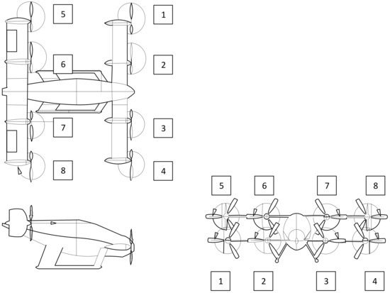
Figure 1.
The appearance and configuration of the dual-tilt-wing eVTOL aircraft selected.
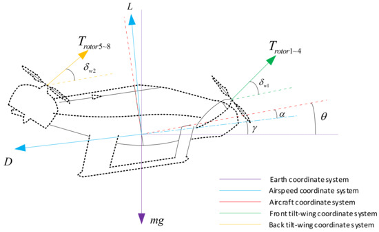
Figure 2.
Longitudinal force diagram of the dual-tilt-wing eVTOL aircraft.
Where is the aerodynamic drag, is the aerodynamic lift, is the tilt angle of the front wing, and is the tilt angle of the rear wing. Here, the tilt angles of the two wings are defined as 0° when parallel to the x-axis of the aircraft coordinate system and 90° when parallel to the z-axis of the aircraft coordinate system. denotes the gravitational force acting on the aircraft. is the angle of attack, is the flight path angle, and is the pitch angle. The numbering of each propeller of the vehicle is shown in Figure 2. Because this paper only deals with the landing of the vehicle under the longitudinal profile, whether the propeller thrust magnitudes on the same tilting wing are the same or different will not directly affect the longitudinal profile of force and moment changes. Therefore, here, the propellers on the same tilting wing are assumed to produce the same thrust by default. The four propellers on the front wing are numbered 1 to 4, so they all produce a thrust of . The four propellers on the rear wing are numbered from 5 to 8, so they all produce a thrust of . The aforementioned angles in the longitudinal plane satisfy the following relationship equation:
The aerodynamic coefficients in [19] are referenced here, and the specific image is shown in Figure 3.
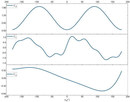
Figure 3.
Values of lift coefficient, drag coefficient, and pitching moment coefficient at different combined angles of approach.
Because the vehicle is a tilt-wing vehicle, its dynamic change process is highly complex. Therefore, here, for the vehicle in different states, the relationship between the combination of the angle of approach, the angle of attack, the tilt-wing angle, and the rudder can be approximated as
As for the specific values of each parameter of the vehicle, they are shown in the fol-lowing Table 1.

Table 1.
Aircraft-related parameters.
As shown in Figure 2, a closer examination of the aircraft’s coordinate system reveals the intricate relationship between the axial overload and the aircraft’s thrust and aerodynamic drag. The normal overload is also determined based on the interaction of aerodynamic lift, gravitational forces, and the pulling force generated by the aircraft. The aircraft’s tilting wing feature introduces a dynamic variable, as the angle of attack of the oncoming airflow relative to the wings is highly sensitive to changes in the wing’s tilt angle. Moreover, adjustments in the wing’s tilt angle considerably alter the aerodynamic pitching moment coefficient, which is crucial for the aircraft’s stability and control. Concurrently, variations in the magnitude and direction of the thrust lead to fluctuations in the moment in the aircraft’s center of gravity, thereby influencing the pitch acceleration. The interaction between the two tilting wing surfaces leads to a complex, simultaneous modulation of axial overload, normal overload, and pitch acceleration, generating a strong coupling effect among the aircraft’s forward motion, vertical movement, and pitch behavior. Because aerodynamic forces are defined within the velocity coordinate system, the composite velocity of the aircraft is initially described as follows:
represents the airspeed of the aircraft, represents the ground speed of the aircraft, and represents the wind speed. The forces and moments in the velocity coordinate system can be represented by the following formulas:
where is the force component along the x-axis of the velocity coordinate system produced by the four propellers on the front wing, is the force component along the x-axis of the velocity coordinate system produced by the four propellers on the rear wing, is the force component along the z-axis of the velocity coordinate system produced by the four propellers on the front wing, and is the force component along the z-axis of the velocity coordinate system produced by the four propellers on the rear wing. represents the pitch moment generated by aerodynamic forces, represents the pitch moment generated by the propellers on the front wing, and represents the pitch moment generated by the propellers on the rear wing. is the net external force in the x-direction of the velocity coordinate system of the aircraft, is the net external force in the z-direction of the velocity coordinate system of the aircraft, and is the net external moment of the y-axis in the aircraft’s body coordinate system. is the number of propellers on the front wing that are functioning normally, and is the number of propellers on the rear wing that are functioning normally. is the distance from the propellers on the front wing to the center of gravity along the x-axis of the body coordinate system, is the distance from the propellers on the front wing to the center of gravity along the z-axis of the body coordinate system, is the distance from the propellers on the rear wing to the center of gravity along the x-axis of the body coordinate system, and is the distance from the propellers on the rear wing to the center of gravity along the z-axis of the body coordinate system.
From the relationship between the velocity coordinate system and the aircraft coordinate system, as well as Equation (6), it can be deduced that
where is the external force on the aircraft in the x-direction of the body coordinate system, excluding gravity, is the external force on the aircraft in the z-direction of the body coordinate system, excluding gravity, and is the net external moment of the y-axis in the body coordinate system of the aircraft. From the above equations, it is possible to solve for the forces and moments acting on the aircraft in the body coordinate system at the next moment.
Assuming that the aircraft’s lateral forces and moments are in balance, its longitudinal dynamics equations are as follows:
where is the displacement of the aircraft in the x-direction of the Earth coordinate system, is the altitude at which the aircraft is currently located, is the velocity of the aircraft in the x-direction of the Earth coordinate system, is the velocity of the aircraft in the z-direction of the Earth coordinate system, and is the pitch rate.
Building upon the kinetic modeling discussed earlier, a set of specific inputs was established for the forces generated by the vehicle’s propellers and the tilt angles of the tilting wings. The objective was to evaluate whether the vehicle’s aggregate external forces and moments could reach equilibrium across various velocities and trajectory tilts. The subsequent analysis presents the trim envelopes for the vehicle under different degrees of power loss on both the front and rear airfoils. Because there are so many combinations of different power losses, only the leveling packages of power intact, 25% power loss, and 75% power loss are considered here, which represent all power intact, one rotor power loss on each of the front and rear wings, and three rotor power losses on each of the front and rear wings, respectively. In the following set of array plots, the horizontal coordinates represent the different power loss levels of the vehicle, and the vertical coordinates represent the magnitude of the rotor thrust on the front wing, the magnitude of the rotor thrust on the rear wing, the front wing’s inclination angle, and the rear wing’s inclination angle. The corresponding values change in magnitude, as indicated by a color change in the individual plots. And, on each subplot, its horizontal coordinate represents the combined velocity of the vehicle and the vertical coordinate represents the trajectory inclination of the vehicle.
From Figure 4, it can be found that the leveling envelope shrinks as the loss of power gradually increases. When the power loss reaches 75%, the leveling envelope only remains near zero track inclination at high speed and near −50° track inclination. If the landing state is considered, the vehicle cannot have a high longitudinal velocity upon touching the ground, so the region of high speed and −50° trajectory inclination is not suitable for the vehicle’s landing. At the same time, when the power is lost by 50%, the aircraft cannot be leveled at low speed. Then, only the area around high speed and 0° track inclination can be used so that the aircraft can be safely landed.
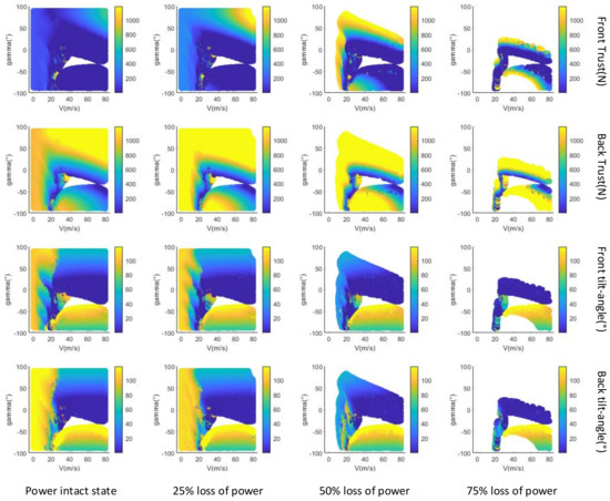
Figure 4.
Trim envelope at different percentages of power loss.
3. Emergency Landing Control Design for eVTOL Aircraft
3.1. The Overall Control Framework
In this study, we have meticulously designed a control architecture, dividing it into five core components, including the command filter module, the control law module, the control allocation module, the aircraft system module, and the sensor module, as shown in Figure 5. The process begins with the sensor module, which captures the aircraft’s state variables from the previous moment and forwards these data to the command filter module. This module then carefully analyzes the landing command, considering the geometric dimensions of the landing field and the operational environment, and divides it into two components: a control target component and a constraints component. The control target component translates the ultimate objective into a set of targets for all state variables, carefully analyzing their interdependencies. In contrast, the constraints component examines the safe operational thresholds for all state variables, analyzing the interplay between airworthiness requirements and the boundaries of each state variable, based on the intended destination.
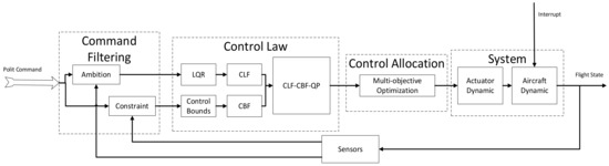
Figure 5.
Overall control framework.
The control law module utilizes the Linear Quadratic Regulator (LQR) method to formulate the control Lyapunov function for the target component. It adeptly incorporates boundary constraints into the control barrier functions by combining the upper and lower limits of each input and assigning diverse weights to the state variables. Subsequently, the quadratic programming (QP) algorithm is utilized to combine the control Lyapunov function with the control barrier functions. This results in the establishment of constraints and the derivation of the optimized total external force and torque command necessary for the aircraft at the next moment. In the control allocation module, the total external force and torque specified by the control law are effectively apportioned to each actuator on the aircraft through a multi-objective optimization framework. These control input commands are then relayed to the actuators, initiating a modification in the aircraft’s flight state. This coordination guides the aircraft to establish and adhere to a safe landing trajectory, thereby achieving the intended control objectives. The specific workflow is illustrated in Figure 6.
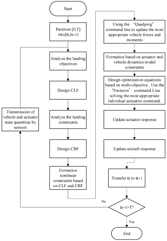
Figure 6.
Flowchart of the operation of the control framework.
From the preceding discussion, it is clear that the command filter module effectively differentiates between desired objectives and state constraints, carefully crafting the control Lyapunov function (CLF) and control barrier functions (CBF). This strategic separation ensures that the aircraft navigates towards the target destination along an optimized trajectory while avoiding any encroachment on obstacle boundaries. Moreover, because both the control law and control allocation are based on optimization algorithms, they remain robust against variations in the model with respect to control goals and obstacle constraints. This attribute significantly reduces the complexity inherent in addressing multi-input, nonlinear, and strongly coupled control challenges. An additional advantage of this control framework is the seamless integration of the aircraft’s landing trajectory planning, guidance, and control mechanisms. It not only complies with landing constraints but also has the agility to dynamically adjust the aircraft’s attitude, flight velocity, and directional orientation in real time. This adaptability is crucial for responding to unforeseen obstacles or disturbances that may arise during the landing sequence. By maintaining this level of responsiveness, the framework ensures that the aircraft can safely and effectively achieve the required control objectives.
3.2. Setting of Control Barrier Functions
Firstly, a nonlinear affine system can be defined as follows:
where is expressed as the state quantity and is expressed as the input quantity. We can construct a barrier function and derive its differential expression as follows:
The CBF can be constructed, which is , and
The above formula can be written as
The intention is to ensure that the barrier function never actually reaches zero. By setting it to be greater than zero, we establish a safety margin between the system’s operational limits and the barrier function itself. This enables the system to respond and adjust its behavior through the barrier function before it approaches the critical boundary. A typical representation of the barrier function is depicted in Figure 7.
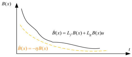
Figure 7.
Barrier function operating mechanism.
The objective is to ensure that the barrier function never approaches zero, thereby maintaining a safe margin between the system’s operational limits and the barrier function itself. This facilitates the system’s proactive response through the utilization of the barrier function prior to reaching critical boundaries, as depicted in Figure 5. Considering the crucial elements involved in a gliding landing, three control barrier functions are judiciously chosen to impose stringent control constraints.
Taking into account the safety of onboard personnel and the aerodynamic and structural integrity of the aircraft during landing, it is essential to establish three control barrier functions. The first of these functions relates to constraining the aircraft’s vertical speed. Given the structural strength limitations of the aircraft and the strict airworthiness requirements, the aircraft must avoid high longitudinal velocities during landing to prevent structural deformation upon touchdown, which could endanger the safety of passengers. Consequently, we define upper and lower bounds for the aircraft’s longitudinal velocity during landing, thereby ensuring that it remains within a safe threshold throughout the landing sequence.
where is the upper boundary of the aircraft’s vertical velocity and is the lower boundary of the vertical velocity. The purpose of setting this barrier function is to ensure that the aircraft does not have a large vertical velocity during the gliding process and to ensure that the aircraft can eventually land safely.
The second control barrier function is devised with the aim of delineating the boundaries for the vehicle’s landing trajectory inclination. Given the vehicle’s minimal speed upon landing and in accordance with the trim envelope represented in Figure 4, in the event of substantial power loss, the vehicle must operate in the vicinity of the high-speed, 0° trajectory inclination segment of the envelope to guarantee a smooth landing. Consequently, it is crucial to establish definitive upper and lower bounds for the vehicle’s trajectory inclination. This ensures that the vehicle can land smoothly while sustaining its equilibrium. This meticulous approach ensures that the vehicle’s descent is controlled and secure, facilitating a stable and manageable trajectory throughout the landing process.
where is the upper boundary of the flight path angle, is the lower boundary of the flight path angle, is the change in altitude within a unit step, and is the change in horizontal displacement within a unit step.
Considering that the flight environment of the aircraft is predominantly urban airspace, obstacles (such as flocks of birds, etc.) are highly likely to appear at any time within the airspace during flight. To ensure the safety of the aircraft during flight, it is highly necessary to integrate elements related to obstacle avoidance into the control barrier function. Here, the control barrier function related to obstacle avoidance is designed in the following manner:
where is the horizontal position of the center of the obstacle, is the vertical position of the center of the obstacle, is the radius of the largest circle that can enclose the obstacle and leave some margin at the same time, and is the coefficient in the barrier function. The purpose of setting this barrier function is to ensure that the aircraft has obstacle avoidance capabilities in the landing environment.
3.3. The Setting of the Control Lyapunov Function
Meanwhile, the Lyapunov function is constructed to ensure that it is always greater than 0 and that it gradually approaches 0 with the increase of time, which is obtained through the following differential expression:
The CLF can be constructed, which is , and
The above formula can be written as
This means that with the increase in time, the virtual energy of the system will gradually decrease, and, in the process, the conditions of to be met are
must be greater than 0 because it is necessary to ensure that the system is always in a stable state; its upper bound is set to ensure that the system can converge according to the set convergence rate, and the size of its convergence rate can be adjusted by changing .
When applied to the system and the application scenarios proposed in this paper, the nonlinear model is linearized. Considering that the aircraft must ensure ride quality during the actual landing, the and are relatively small, so Equation (2) is simplified. The differential term of the velocity can be simplified as follows:
After simplification, the dynamics equation can be regarded as a linear system, as shown in the following formula:
where represents the state vector, represents the input vector, and represents the output vector. Here, a method based on the LQR (the Linear Quadratic Regulator) is adopted to ensure that the path to the desired position of the flight is optimal. Given the weight matrices and , the control law can be derived from the theory of the LQR controller as follows:
where represents the state feedback matrix and represents the auxiliary matrix in the LQR (the Linear Quadratic Regulator) controller theory. According to this theory, when is minimized, the value of the cost function in the LQR is minimized. Using MATLAB (2024a) software, when given the determined , , , , and arrays, the P array can be derived directly. After debugging, the values of the and arrays set here are
Therefore, a Lyapunov equation is constructed using the matrix as follows:
Because the aircraft is in the process of gliding down at this point, the desired state is set here as follows:
The significance of the characterization lies in the fact that the horizontal and vertical velocities of the vehicle are constantly changing with altitude, while the attitude angle of the vehicle remains stable and the vehicle is always flying towards the origin of the reference coordinate system. By the time of final landing, the desired landing speed of the vehicle is approximately 25 m/s in the horizontal direction and 0.1 m/s in the vertical direction.
Because the matrix is a positive definite quadratic form matrix, is always greater than 0.
The derivative of is shown as follows:
By substituting Equation (22) into the previous equation, further derivation can be achieved as follows:
Because the matrix here is the identity matrix, it follows that
This meets the theoretical requirement.
According to the given CLF and CBF, the CLF-CBF-QP comprehensive constraint function can be constructed as follows:
where is the QP weight diagonal matrix, whose value is the weight ratio for different input quantities. The function of the loose variable is to release the soft constraint on the CLF, and represents the weight of this loose variable, while represents the set of inputs that can be reached.
When there may be multiple obstacles in the system, that is, multiple barrier functions are required to constrain the quadratic programming of the aircraft at the same time, then the function needs to be rewritten as
where is the first control barrier function, is the second control barrier function, and so on.
3.4. Control Allocation Based on Optimization
The control allocation design uses a decentralized search mechanism to generate multiple starting points within the limit range, which are then substituted into the optimization function. The interior point method is used to find the solution that minimizes the optimization function, and this set of solutions is the vector of control inputs for the aircraft. The control inputs include , , , and . The five optimization objectives selected here are the minimum thrust, the minimum difference in tilt angles between the front and rear wings, the minimum elevator deflection angle, and the minimum change in tilt angle of the wing over a single step.
where , , and are three parameters in the optimization function, is the net external force along the x-axis in the body coordinate system calculated from the solution of the optimization function, and is the net external force along the z-axis in the body’s coordinate system calculated from the solution. Based on this framework, is the net external moment of the y-axis in the body’s coordinate system calculated using the solution of the optimization function. By adjusting the parameters to change the importance of different optimization objectives, the combination of control input magnitudes for each moment can ultimately be obtained.
4. Simulation Verification
In order to verify the validity of the proposed method in guaranteeing the safety and performance of the target aircraft within complex environments, a suite of simulation tests has been performed. These simulations are designed in accordance with airworthiness regulations and comprise three distinct scenarios: (1) glider landing of the aircraft under different degrees of power loss, (2) landing trajectory in the presence of obstacles in the airspace, and (3) emergency landing in a different initial position. The vehicle modeling, controller design, etc. are simulated using MATLAB. Taking the simulation verification in Section 4.1 as an example, the vehicle takes approximately 225 s to land in the simulation, whereas the entire code takes about 47 s to run through the computer.
4.1. Glider Landing of the Aircraft Under Different Degrees of Power Loss
Here, the initial point of the aircraft is selected as (−6000, 150), with a forward flight speed of 30 m/s for controlling the aircraft. The upper boundary of the obstacle is defined by a flight path angle of 5°, located at a distance of 800 m from the ground, and the lower boundary of the obstacle is defined by a flight path angle of 1°, located at a distance of −800 m from the ground. The allowable landing range on the ground is from −800 m to 800 m.
The following are the actuator responses of the aircraft under different degrees of power loss, where and represent the thrust responses of individual propellers on different wings of the aircraft.
From the above figure, it can be seen that the state quantity response during the landing process of the vehicle is consistent. However, when the vehicle is in different power loss states, there are still some differences in its response. Figure 8 shows the landing trajectory at this initial position, and the vehicle can eventually land with a small trajectory inclination. Figure 9 shows the response of each state quantity. When it is about to land, the velocity of the vehicle in the horizontal direction is around 25 m/s, the velocity in the vertical direction is around 0.2 m/s, the attitude angle is stabilized at 2°, and the attitude angular velocity is stabilized at 0°/s. Figure 10 shows the control input response. It can be seen that when the flight is in a steady state, the force and moment of the vehicle are stabilized at a certain value and no longer change more drastically. Figure 11 represents the response of the actuator after the front and rear wings are lost to different degrees at the same time, and it can be seen that the response of its tilting airfoil angle is still basically the same. However, the power will be lost due to the power loss of some of these propellers, thus requiring other propellers to provide some supplementation. Figure 12 looks for the maximum degree of power loss on one airfoil after the complete loss of power on the other airfoil. It can be found that due to the loss of power on one airfoil, the remaining propellers on the other airfoil need to increase the power, and the airfoil with complete loss of power needs to increase the tilt angle to ensure that the vehicle can achieve the balance of forces and moments.
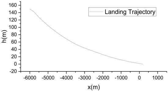
Figure 8.
Aircraft emergency landing trajectory.
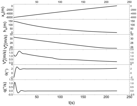
Figure 9.
Response curves of various state quantities for aircraft emergency landing.
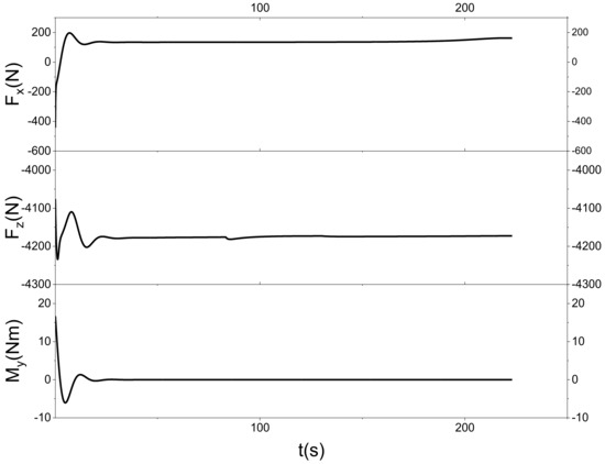
Figure 10.
Response curves of aircraft control inputs.
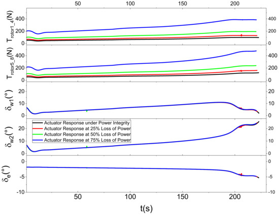
Figure 11.
Response curves of various aircrafts under different degrees of power loss 1.
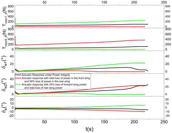
Figure 12.
Actuator response levels under various degrees of power loss 2.
4.2. Landing Trajectory in the Presence of Obstacles in the Airspace
Here, two obstacles are set up, both with their centers located at (−3200, 50), with radii of 10 m and 20 m, respectively.
Figure 13 characterizes the landing trajectory of the vehicle when there are different sizes of obstacles in the airspace. Before the vehicle is about to reach the obstacle, due to the existence of the third function of the CBF, the vehicle will go around from the top of the obstacle and then proceed to land, but the landing will be deviated from the established landing point by a certain distance. Figure 14 shows the local zoomed-in image, and it is found that the landing trajectory of the vehicle cannot cross the boundary line of the obstacle. Figure 15 shows the response curve of each state quantity, and it can be found that the vertical velocity will have a larger magnitude in advance before it is about to encounter the obstacle. Figure 15 also shows the response curves of each state quantity, and it can be seen that the vertical velocity of the vehicle will be reduced greatly in advance before hitting the obstacle so as to ensure that the vehicle can go around the obstacle in an approximately horizontal forward flight. Figure 16 shows the response of the vehicle’s angle of attraction and trajectory inclination, and, when hitting the obstacle, the vehicle’s angle of attraction and trajectory inclination will be reduced to a certain extent. Figure 17 shows the vehicle control input response. In the presence of obstacles, the force and moment of the vehicle will have a smaller response, because the force and moment of the vehicle will directly change the linear acceleration and rotational acceleration of the vehicle, and this change needs to be integrated over time to be reflected in the velocity and position of the vehicle. Figure 18 shows the response curves of each actuator of the vehicle. Due to the long flight time of the vehicle, the response of the actuator with and without obstacles is mainly reflected in the change of the tilt-wing. It has been observed that within the framework of this control system, the aircraft is capable of efficiently avoiding obstacles that appear along the original landing trajectory. The aircraft can adjust its trajectory in response to the size of the obstacles, thereby ensuring that it can navigate around them effectively and ultimately meet the landing requirements.
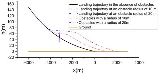
Figure 13.
Landing trajectory with obstacles present in the airspace.
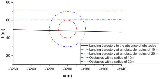
Figure 14.
Landing trajectory with obstacles present in the airspace (enlarged view).
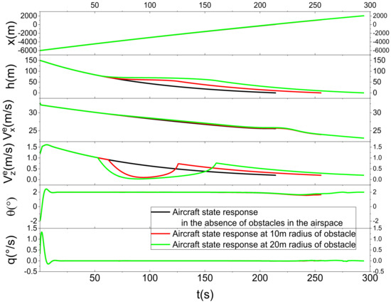
Figure 15.
Response curves of state quantities when obstacles are present in the airspace.
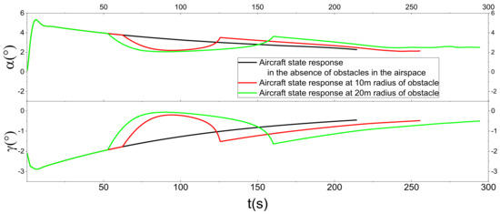
Figure 16.
Angle of attack and flight path angle response curves with obstacles in the airspace.
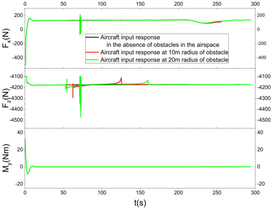
Figure 17.
Control input response curves in the presence of obstacles in the airspace.
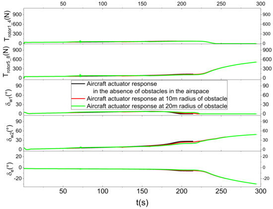
Figure 18.
Actuator response curves in the presence of obstacles in the airspace.
4.3. Emergency Landing in Different Initial Position
Here, six different initial points are selected, each with a position in the airspace of (−7000, 150), (−6000, 180), (−6000, 120), (−6000, 100), (−5000, 180), and (−5000, 100). Using the same set of control frames and set to the same set of parameters, the following is the landing effect of the aircraft.
Figure 19 shows that the vehicle can fulfill the landing requirements at different initial points. Figure 20 shows that the horizontal and vertical velocities of the vehicle are stabilized within a certain range when it is about to land, and it is reasonable to land at this range of velocities. Figure 21 shows that the control inputs of the vehicle are all stabilized near the same value eventually. Figure 22 shows that the thrusts on the front wings are all reduced when it is about to land, the thrusts on the rear wings are all increased, and the front and rear wings change accordingly. When landing, the thrust on the front wing of the vehicle will decrease, the thrust on the rear wing will increase, and the front and rear wings will change accordingly. It can be found that with the same set of control parameters, the aircraft can land safely from different initial points and meet the requirements within a certain range. It can thus be seen that the method is robust.
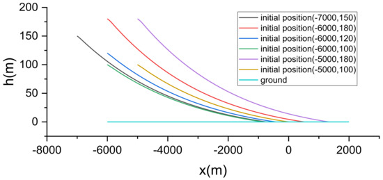
Figure 19.
Landing trajectories with different initial point states.
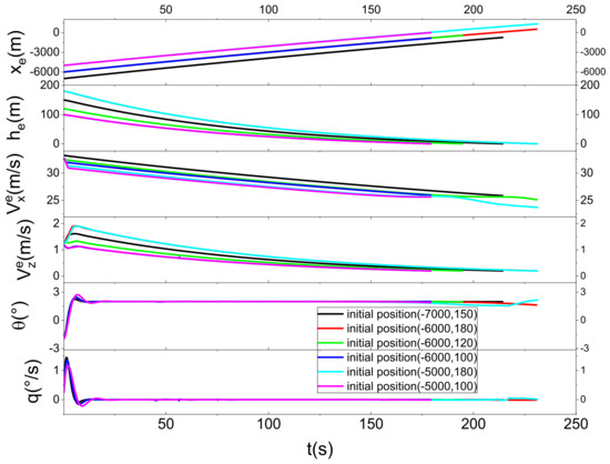
Figure 20.
State response with different initial point states.
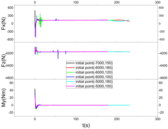
Figure 21.
Input response with different initial point states.
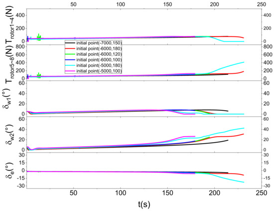
Figure 22.
Actuator response with different initial point states.
5. Conclusions
This paper presents a highly sophisticated and meticulously engineered control framework designed to expertly guide a tilt-wing EVTOL aircraft through the intricate process of safe descent to the ground during emergency gliding landing missions within the dynamic domain of Urban Air Mobility (UAM). The framework has been constructed with an astute consideration of the exacting landing requirements, which are rigorously dictated by the aircraft’s robust structural design and the omnipresent threat of potential aerial obstacles within urban airspace. It ingeniously incorporates an advanced obstacle function, leveraging state-of-the-art quadratic programming techniques to formulate the control laws with utmost precision and in a highly systematic and methodical fashion.
Through an extensive series of comprehensive simulations, meticulously designed across three distinct and judiciously selected scenarios, the safety and efficacy of this control framework have been subjected to rigorous evaluation and exhaustive testing. The simulation results, which are the culmination of extensive research and computational efforts, unequivocally demonstrate that the proposed framework not only ensures the secure execution of emergency gliding landings but also showcases an exemplary and exceptionally robust performance. This outstanding performance underscores the framework’s capacity to adeptly navigate through the most challenging circumstances, thereby unequivocally demonstrating its superiority and unwavering reliability in handling various unpredictable and demanding conditions.
This innovative approach represents a significant stride forward in the realm of autonomous emergency gliding landing guidance and control for tilt-wing eVTOLs, addressing the critical need for safe operations in UAM missions. By integrating CBFs, the proposed framework offers a novel and effective solution to the complex problem of safely guiding aircrafts in urban environments, characterized by a multitude of obstacles and ever-changing conditions. It not only enhances our understanding of emergency landing mechanisms for eVTOLs but also makes a substantial contribution to the broader field of urban air traffic management. This research lays a solid foundation for future investigations and practical implementations, setting a new benchmark for resilient aircraft control in complex urban scenarios. The seamless combination of CBFs and global optimization techniques marks a paradigm shift, opening up new vistas for the safe integration of eVTOLs into the fabric of everyday urban life, thus revolutionizing urban transportation through the innovative applications of electric Vertical Take-Off and Landing (eVTOL) aircraft.
Author Contributions
Validation, L.M.; Resources, L.M.; Data curation, Y.D.; Writing—original draft, Y.D.; Writing—review & editing, J.Y. All authors have read and agreed to the published version of the manuscript.
Funding
This research was funded by Civil Aviation University of China grant number [3122024046].
Data Availability Statement
The data that support the findings of this study are available on request from the corresponding author, upon reasonable request.
Conflicts of Interest
The authors declare no conflict of interest.
References
- Reiche, C.; McGillen, C.; Siegel, J.; Brody, F. Are We Ready to Weather Urban Air Mobility (UAM)? In Proceedings of the 2019 Integrated Communications, Navigation and Surveillance Conference (ICNS), Herndon, VA, USA, 9–11 April 2019; pp. 1–7. [Google Scholar] [CrossRef]
- Melo, S.P.; Cerdas, F.; Barke, A.; Thies, C.; Spengler, T.S.; Herrmann, C. Life Cycle Engineering of future aircraft systems: The case of eVTOL vehicles. Procedia CIRP 2020, 90, 297–302. [Google Scholar] [CrossRef]
- May, M.S.; Milz, D.; Looye, G. Semi-Empirical Aerodynamic Modeling Approach for Tandem Tilt-Wing eVTOL Control Design Applications. In Proceedings of the AIAA SCITECH 2023 Forum: American Institute of Aeronautics and Astronautics, National Harbor, MD, USA, 23–27 January 2023. [Google Scholar]
- Federal Aviation Administration. Airworthiness Criteria: Special Class Airworthiness Criteria for the Joby Aero, Inc. Model JAS4-1 Powered-Lift; FAA: Washington, DC, USA, 2022.
- European Union Aviation Safety Agency. Proposed Means of Compliance with the Special Condition VTOL (Doc. No: MOC SC-VTOL, Issue 1). 2020. Available online: https://www.easa.europa.eu/en/document-library/product-certification-consultations/special-condition-vtol (accessed on 3 November 2024).
- Li, P.; Chen, X.; Li, C. Emergency landing control technology for UAV. In Proceedings of the 2014 IEEE Chinese Guidance, Navigation and Control Conference, Yantai, China, 8–10 August 2014; pp. 2359–2362. [Google Scholar] [CrossRef]
- Fang, X.; Jiang, J.; Chen, W.-H. Model Predictive Control with Wind Preview for Aircraft Forced Landing. IEEE Trans. Aerosp. Electron. Syst. 2023, 59, 3995–4004. [Google Scholar] [CrossRef]
- Lee, I.R.; Choi, Y.S.; Lim, M.G.; Woo, J.W.; Kim, C.J. Guidance and control for autonomous emergency landing of the rotorcraft using incremental backstepping controller in 3D terrain environments. Aerosp. Sci. Technol. 2023, 132, 108051. [Google Scholar] [CrossRef]
- Procházka, O.; Novák, F.; Báča, T.; Gupta, P.M.; Pěnička, R.; Saska, M. Model predictive control-based trajectory generation for agile landing of unmanned aerial vehicle on a moving boat. Ocean Eng. 2024, 313, 119164. [Google Scholar] [CrossRef]
- Park, J.; Kim, I.; Suk, J.; Kim, S. Trajectory optimization for takeoff and landing phase of UAM considering energy and safety. Aerosp. Sci. Technol. 2023, 140, 108489. [Google Scholar] [CrossRef]
- Fang, X.; Benzerrouk, H.; Landry, R.J. Energy Management and Guidance for Gyroplane Autonomous Unpowered Landing Based on Onboard Trajectory Generation. IFAC-PapersOnLine 2019, 52, 250–255. [Google Scholar] [CrossRef]
- Tang, P.; Zhang, S.; Li, J. Final Approach and Landing Trajectory Generation for Civil Airplane in Total Loss of Thrust. Procedia Eng. 2014, 80, 522–528. [Google Scholar] [CrossRef]
- Fang, X.; Wang, Y.; Landry, R.J. Onboard trajectory generation for gyroplane unpowered landing based on optimal lift-to-drag ratio target. Aerosp. Sci. Technol. 2018, 82–83, 438–449. [Google Scholar] [CrossRef]
- Jie, B.; Xu, Z. Research on Over-Speed Protection Control Method for Aircraft Engines Based on Control Barrier Functions. In Proceedings of the 7th International Conference on Advanced Algorithms and Control Engineering (ICAACE), Shanghai, China, 1–3 March 2024; pp. 1233–1237. [Google Scholar] [CrossRef]
- Wang, K.; Meng, T.; Wang, W.; Lei, J. Control barrier function based trajectory generation and tracking control for spacecraft inspection mission under multiple safety constraints. Adv. Space Res. 2024, 73, 2080–2097. [Google Scholar] [CrossRef]
- Farras, A.W.; Hatanaka, T. Safe Control with Control Barrier Function for Euler-Lagrange Systems Facing Position Constraint. In Proceedings of the 2021 SICE International Symposium on Control Systems (SICE ISCS), Tokyo, Japan, 2–4 March 2021; pp. 28–32. [Google Scholar] [CrossRef]
- Li, B.; Wen, S.; Yan, Z.; Wen, G.; Huang, T. A Survey on the Control Lyapunov Function and Control Barrier Function for Nonlinear-Affine Control Systems. IEEE/CAA J. Autom. Sin. 2023, 10, 584–602. [Google Scholar] [CrossRef]
- Long, K.; Dhiman, V.; Leok, M.; Cortes, J.; Atanasov, N. Safe Control Synthesis with Uncertain Dynamics and Constraints. IEEE Robot. Autom. Lett. 2022, 7, 7295–7302. [Google Scholar] [CrossRef]
- May, M.S.; Milz, D.; Looye, G. Dynamic Modeling and Analysis of Tilt-Wing Electric Vertical Take-Off and Landing Vehicles. In Proceedings of the AIAA SCITECH 2022 Forum: American Institute of Aeronautics and Astronautics, San Diego, CA, USA, 3–7 January 2022. [Google Scholar]
Disclaimer/Publisher’s Note: The statements, opinions and data contained in all publications are solely those of the individual author(s) and contributor(s) and not of MDPI and/or the editor(s). MDPI and/or the editor(s) disclaim responsibility for any injury to people or property resulting from any ideas, methods, instructions or products referred to in the content. |
© 2025 by the authors. Licensee MDPI, Basel, Switzerland. This article is an open access article distributed under the terms and conditions of the Creative Commons Attribution (CC BY) license (https://creativecommons.org/licenses/by/4.0/).