LEO Satellite Navigation Based on Optical Measurements of a Cooperative Constellation

Abstract

Autonomous, anti-jamming, and high-precision satellite navigation are of great importance to current and future space technologies. This paper proposes a cooperative constellation navigation system for low Earth orbit (LEO) satellites that use only the optical measurements of cooperative satellites. Based on photometry, an optical transmission link model of the system is built. With the pixel coordinates of the cooperative satellites on the optical images, the line of sight (LoS) vectors of the cooperative satellites with respect to the LEO spacecraft are first calculated, and a single-point positioning method based on the LoS vectors’ inner products is proposed. The single-point positioning results are then fed into a least square batch filter to estimate a high-precision spacecraft orbit. Simulations are conducted to evaluate the potential navigation accuracy. With a cooperative satellite ephemeris error of 100 m and an optical measurement noise level of 5 arcsecs, position accuracies of single-point positioning and dynamic orbit determination in the order of hundreds of meters and eight meters, respectively, are realized. In addition, the influences of the orbital altitude of the cooperative constellation, the ephemeris error of the cooperative satellite, the noise level of the optical measurements, and the Earth’s gravitational model on navigation accuracy are investigated via comparative simulations.

1. Introduction

In the early era of space exploration, satellite navigation relied on ground tracking stations. The available measurements from ground stations include the ranges, bearings, and radio signal Doppler frequency shifts of the satellite with respect to the ground station. A representative historical system is the Minitrack system introduced in the late 1950s, which provided angle observations and was used to track Vanguard satellites [1]. Ground-based satellite navigation has the merits of high precision and high reliability and still plays an irreplaceable role in modern space missions.

With the rapid development of space technology, the number of artificial Earth satellites has increased explosively. To date, more than 10,680 satellites have been launched by humankind, and about 6250 satellites are now operating in orbit [2]. The large number of satellites in orbit has introduced a great burden to ground facilities. In addition, ground-based satellite navigation usually cannot be done in real time, as a ground facility cannot track a satellite on the opposite side of the Earth. The Global Positioning System (GPS) is currently the most popular autonomous satellite navigation method. GPS relies on geometric measurements of the relative distance and direction via the use of electromagnetic waves and can provide real-time and centimeter-level navigation results for low Earth orbit (LEO) satellites [3,4]. However, the electromagnetic wave signals of GPS can be easily jammed or spoofed [5].

In recent years, autonomous satellite navigation in GPS-denied environments has received increasing interest. A representative example is the optical measurement-based autonomous navigation method, as optical signals could not be easily interfered with. A series of autonomous navigation methods based on optical measurements have been proposed, including celestial navigation [6,7,8], optical navigation with landmarks [9,10,11], and inter-satellite link-based navigation [12,13]. The celestial navigation system plays a significant role in optical navigation. Positioning accuracy ranging from tens of meters to a hundred meters can be achieved for LEO satellites via the indirect measurement of stellar refraction. [6,8]. Landmark-based optical navigation methods have also become widely applied to soft landings on planets [10]. Using images of the morphological features or landmarks on the surface of a planet, position and attitude accuracies of 25 m and 0.42 deg, respectively, can be realized. In 2018, Hayabusa2 performed two landing operations successfully using artificial-landmark-based autonomous optical navigation [13]. Work on inter-satellite link-based navigation was first conducted by Markley and Psiaki, who proposed an orbit determination method based on inter-satellite relative position measurements between two satellites [12]. The relative position measurement contains both the range and the LoS information, which are provided by a laser range finder and an optical sensor, respectively. Apart from the above applications, optical measurements have also been adopted for the surveillance of geosynchronous Earth orbit (GEO) objects. It has been demonstrated that optical measurements from the optical sensors onboard a LEO satellite platform offer great benefits for observing GEO objects [14,15].

Based on optical measurements, Hu et al. proposed a new navigation system for LEO satellites using cooperative GEO satellites [16]. Position accuracies of 50 meters were obtained under the condition that the attitude of the LEO satellites was known. This navigation system improved the autonomy of LEO satellites and reduced their dependence on ground facilities. However, in his work, the orientation of the optical sensor had to move along GEO satellites, which necessitated high requirements for the servo-tracking capabilities of the sensors. In addition, a priori attitude information was required to obtain angle measurements in the inertial frame. The present study extends Hu’s work and eliminates the requirements of strict attitude control and a priori attitude information.

This paper is mainly a proof-of-concept study of a cooperative constellation navigation system (CCNS). The main contribution of this paper is as follows. First, a cooperative constellation navigation system is proposed. Owing to the cooperative constellation, the star tracking mode is adopted to replace the target tracking mode and does not require attitude servos for the sensor. Second, an optical transmission link model for the CCNS is built, and the feasibility of the CCNS is verified. Third, a positioning method based on the LoS vectors’ inner products is given. Pixel information is introduced as a measurement in this method instead of right ascension and declination. The proposed positioning method functions independently from a priori attitude information. Finally, the feasibility and performance of the CCNS are demonstrated via simulations.

In this paper, a new navigation method for LEO satellites based on optical measurements of a cooperative constellation is proposed. It is assumed that a cooperative medium Earth orbit (MEO) satellite constellation similar to a GPS constellation is constructed. Cooperative satellites carry optical sources, which actively emit modulated and coded light signals. With the optical sensor onboard the LEO satellite, a light signal can be detected. The information on the cooperative satellite, including ephemeris, light signal emission time, and pixel coordinates of cooperative satellites on the optical images, can be extracted. The pixel coordinate observations are transferred to equivalent LoS vectors, and a single-point positioning method with the LoS vectors’ inner product is developed to directly solve the position of the LEO satellite. Then, iterated least square (ILS) batch filtering with single-point positioning results as inputs is used for precise orbit determination (OD). Finally, a variety of simulations is conducted to analyze the effects of several important factors on navigation accuracy.

The remainder of this paper is organized as follows. Section 2 briefly introduces the segments and working principles of the cooperative constellation navigation system (CCNS). Section 3 analyzes the optical transmission link. Section 4 presents the orbital dynamic model, the optical observation model, and the linearized perturbation model of the LoS vectors’ inner product. Section 5 provides a detailed navigation algorithm, which consists of two parts: the single-point positioning with the LoS vectors’ inner product and the precise orbit determination with the iterated least square method. In Section 6, simulations are developed to demonstrate the feasibility and performance of the CCNS. The conclusions of this study are presented in Section 7.

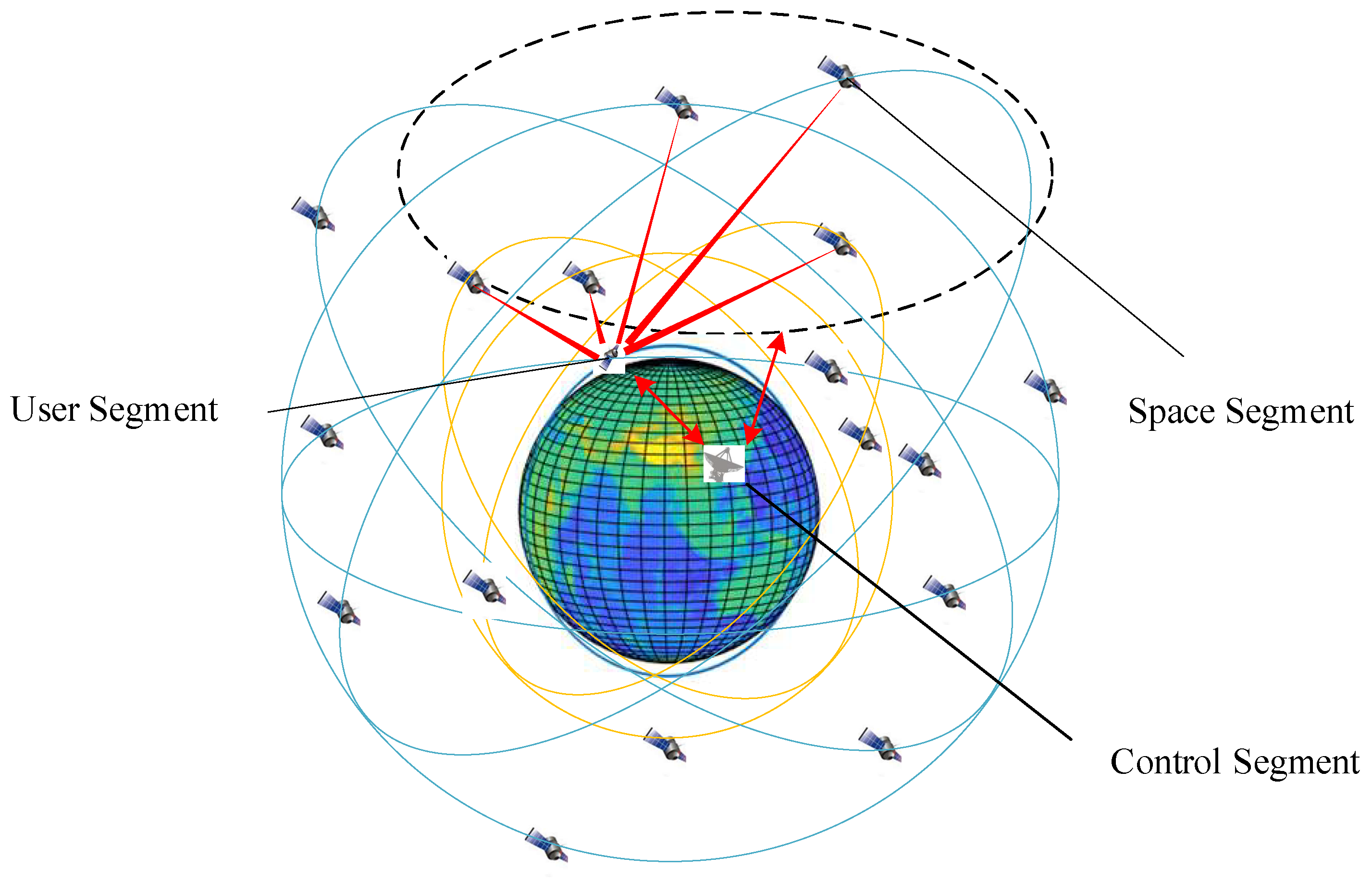
2. Basic Concepts of Cooperative Constellation Navigation System

As shown in Figure 1, the CCNS consists of three segments: the space segment, the user segment, and the control segment. The functions of each segment are as follows.

Figure 1. Overview of CCNS segments.

2.1. Space Segment

The cooperative constellation is similar to that of GPS and consists of 54 cooperative satellites, which move along nearly circular orbits deployed in six evenly spaced planes. Each orbital plane has an inclination of 55° and 12 satellites per plane [17]. Every cooperative satellite is equipped with light sources that can emit a modulated and encoded light signal. The light signal contains the required information for cooperative satellites, including the satellite identification number, ephemeris, light signal emit time, etc. In addition, the cooperative satellites receive uplinked commands and upload them from the control segment, crosslink commands and upload them within the space segment, and downlink optical information to the user segment [18].

2.2. User Segment

The user segment is comprised of satellites in low earth orbits, which are equipped with optical sensors. The user segment’s interaction with the CCNS is achieved through the active optical detection of optical sources mounted on cooperative satellites, which derive optical measurements. Optical sensors adopt the star tracking mode as the observation mode. The aim of using this mode is to observe cooperative satellites as much as possible. The observed cooperative satellites pass through the field of view (FOV) of the optical sensors.

2.3. Control Segment

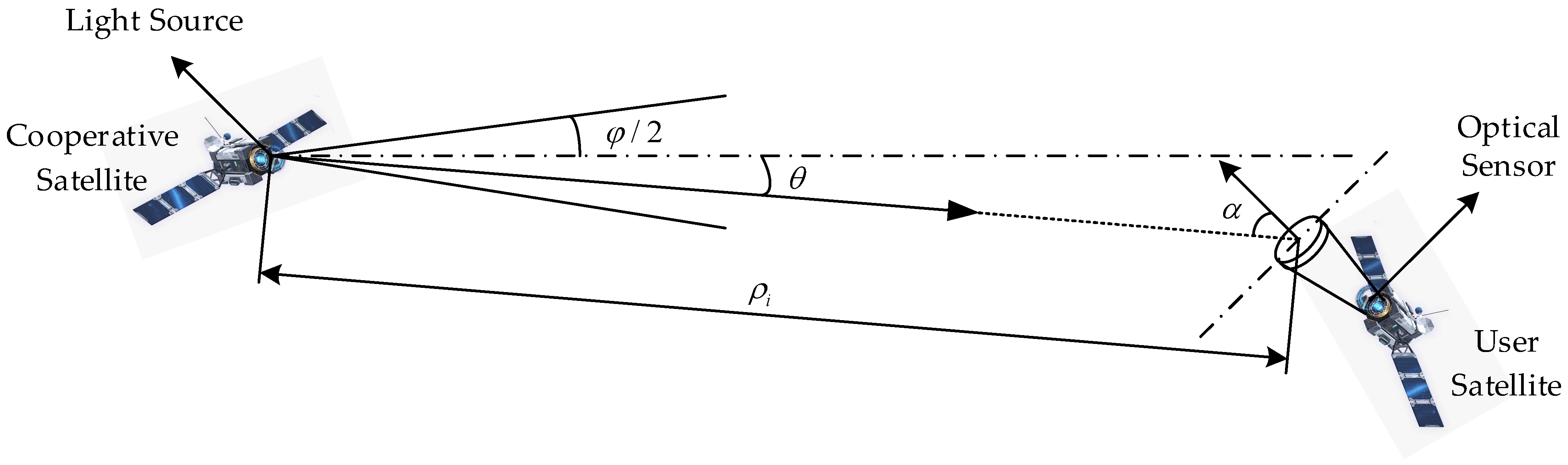
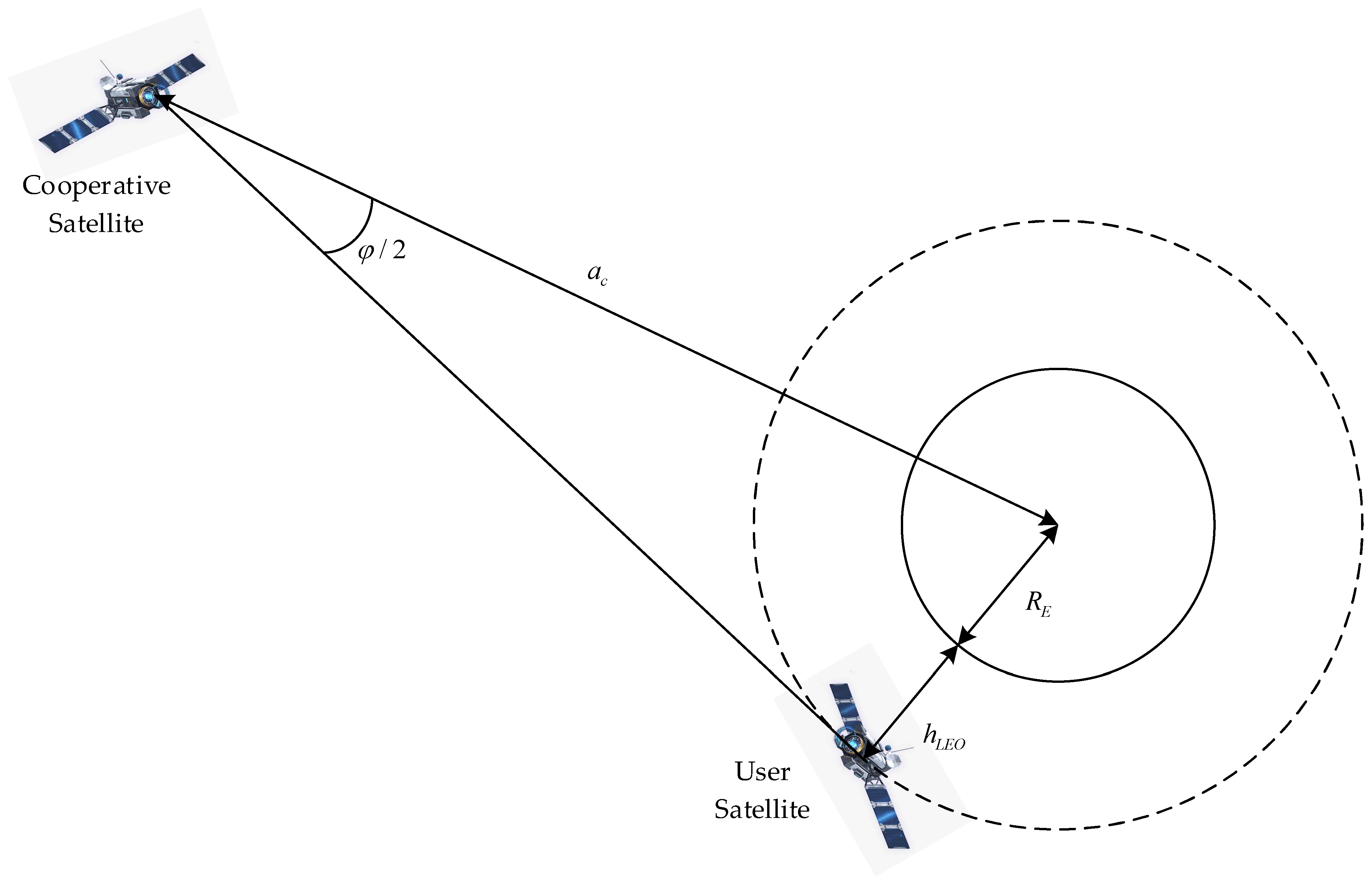
The operational control segment consists of a master control station, monitoring stations, and ground antennas. The main operational tasks of the operational control segment are as follows: tracking the cooperative satellites for the orbit, clock determination, and prediction, and uploading the precise ephemeris of the cooperative satellites to the user segment.

The principle of the CCNS is as follows. With support from the control segment, the ephemeris of cooperative satellites can be obtained and sent to the user segment. In the navigation process, the user satellite’s camera continuously takes photographs of the sky and detects cooperative satellites. From consecutive images, the detected cooperative satellite identification number and corresponding pixel coordinates can be extracted. Then, with pixel coordinates and ephemeris information, the real-time position of the user satellite can be estimated via the single-point positioning algorithm. Finally, the batch least square method is adopted to solve the dynamic orbit determination problem, thereby realizing high-precision spacecraft navigation.

The main acronyms used in this paper are summarized in Table 1 for quick reference.

Table 1. The main acronyms.

Acronym	Description
LEO	Low Earth orbit
LoS	Line of sight
GPS	The Global Positioning System
CCNS	Cooperative constellation navigation system
MEO	Medium Earth orbit
ILS	Iterated least squares
FOV	Field of view
SNR	Signal to noise ratio
ECI	The Earth centered inertial coordinate frame
DOP	Dilution of precision
RMS	Root mean square
OD	Orbit determination

3. Analysis of Optical Transmission Link

3.1. Effective Optical Signals

In a cooperative constellation navigation system, optical radiation is transmitted from the light sources of cooperative satellites to the optical sensors of user satellites through a free space channel (see Figure 2). The basic equation of radiation transfer involves the radiance of the source, the areas of the receiver, and the distance between them [19]. The radiation flux of optical signals emitted by the i^th cooperative satellite at the entrance pupil of the camera can be described as follows:

$${\varphi }_i=\frac{P_i{S}_c\cos \theta \cos \alpha }{4\pi {\sin }^2(\frac{\phi }{4}){\rho }_i{}^2}$$

(1)

where $P_i$ is the optical power of the light source of the i^th cooperative satellite, $S_c$ is the effective receiving area of the optical sensor, ${\rho }_i$ is the distance between the i^th cooperative satellite and the user satellite, $\theta$ is the radiation angle for the light source, $\alpha$ is the incident angle at the optical sensor, and $\phi$ is the divergence angle of the light source.

Figure 2. Diagram of the optical transmission link.

As shown in Figure 3, to ensure full coverage of optical navigation signals to LEO satellites, the divergence angle of the light source $\phi$ should meet the following constraints:

$$\phi \ge 2\arcsin (\frac{R_E+h_{LEO}}{a_c})$$

(2)

where $R_E$ is the earth radius, $a_c$ is the semi-major axis of the cooperative satellite, and $h_{LEO}$ is the orbital altitude of the user satellite. In order to achieve communication coverage of the LEO satellites, $h_{LEO}$ is set to a maximum of 2000 km.

Figure 3. Diagram of Optical Signal Coverage.

To enhance optical signal directivity and reduce the energy divergence of the optical signal, the divergence angle of the light source is set to a minimum value:

$${\phi }_{\min }=2\arcsin (\frac{R_E+h_{LEO}}{a_c})$$

(3)

It can be seen from Equation (3) that the minimum divergence angle of the light source is inversely proportional to the semi-major axis of the cooperative satellite.

Then, electrons converted by the optical radiation flux through the sensor can be calculated as:

$$N_{si}=\frac{{\tau }_0\epsilon Q_s{t}_{\mathrm{int}}{\varphi }_i}{(hc/\lambda )M_{xy}}$$

(4)

where $h$ is the Planck constant; $c$ is light speed; $\lambda$ is the wavelength; ${\tau }_0$, $\epsilon$, $Q_s$, and $t_{\mathrm{int}}$ are the inherent parameters of the camera; ${\tau }_0$ is the spectral transmittance; $\epsilon$ is the fill factor pixel; $Q_s$ is the quantum efficiency; $t_{\mathrm{int}}$ is the integration period; and $M_{xy}$ is the pixel occupied by the star point of the i^th cooperative satellite on the sensor.

According to the Johnson criterion, if 5~10 pixels can be observed for a single star point on the sensor array, the cooperative satellite can be identified. Therefore, $M_{xy}$ is set to 5 in this paper.

Equations (1) and (4) form the channel model of the CCNS for LEO satellite navigation in a space environment. Notably, the CCNS can provide navigation information for aircraft and ground vehicles. In these cases, a more complex channel model considering optical signal link losses and transmission latency should be adopted [20,21].

3.2. Noise Analysis

The main noise sources of the imaging system include photon noise, dark current noise, fixed pattern noise, readout noise, reset noise, amplifier noise, quantization noise, 1/f noise, quantification noise, etc. In this paper, the dominant noise sources are discussed. These sources include photon noise, dark current noise, and readout noise.

3.2.1. Photon Noise

Photon noise occurs due to the random characteristics of the incident electrons, which include background photon noise and target signal photon noise.

The target signal photon noise can be calculated as:

$$n_s=\sqrt{N_s}$$

(5)

The radiation flux of the deep-space background at the entrance pupil of the camera can be described as follows:

$${\varphi }_B=2.9\times {10}^{-8}\times {2.512}^{-M_V}\times S_c$$

(6)

where $M_V$ is the magnitude of the deep-space background, which is normally set to 23.

Electrons generated by background radiation can be calculated as:

$$N_B=\frac{{\tau }_0\epsilon Q_s{t}_{\mathrm{int}}{\varphi }_B}{(hc/\lambda )M}$$

(7)

where $M$ is the total pixels of the imaging area.

Then, the background photon noise can be calculated as:

$$n_B=\sqrt{N_B}$$

(8)

Photon noise follows a Poisson distribution, so it can be calculated as:

$$n_p=\sqrt{n_s^2+n_B^2}$$

(9)

3.2.2. Dark Current Noise

Dark current noise is mainly caused by the thermal motion of charge carriers. Dark current noise is roughly addressed as white noise and follows a Poisson distribution. Its equivalent electrons are the square root of electrons generated by a dark current. Therefore, dark current noise can be calculated as:

$$n_d=\sqrt{N_d}$$

(10)

where $N_d$ represents the electrons generated by the dark current.

3.2.3. Readout Noise

Readout noise, denoted by $n_r$ is mainly caused by random fluctuations in the signal level of the column amplifier, gain amplifier, ADC, etc. The value of readout noise is generally at the level of several to dozens.

To this end, the full noise model of the imaging system can be described as:

$$n_{noise}=\sqrt{n_p^2+n_d^2+n_r^2}$$

(11)

3.3. Signal to Noise Ratio

The signal to noise ratio (SNR) can be used as a criterion to judge whether a cooperative satellite can be detected. According to the basic theory of SNR calculation, the SNR of the imaging system can be expressed as:

$$SNR=\frac{N_s}{n_{noise}}$$

(12)

In order to effectively extract the target signal and reduce the false alarm probability, the SNR must meet the threshold signal to noise ratio limit:

$$SNR\ge SN{R}_0$$

(13)

where $SN{R}_0$ is the threshold SNR determined by the detection probability and false alarm probability. In this paper, the threshold $SN{R}_0$ is empirically set to 5 [22].

4. Orbit Determination Models

4.1. Orbital Dynamic Model

The user satellite’s orbital motion is described by the following first-order differential equation:

$$\frac{d}{dt}\left[\begin{array}{c}R\\ V\end{array}\right]=\left[\begin{array}{c}V\\ a\left(t,R,V\right)\end{array}\right]$$

(14)

where $R$ and $V$ are the user satellite’s position and velocity vectors, and $a\left(t,R,V\right)$ is the acceleration in the Earth-centered inertial (ECI) coordinate frame. Given the initial state (position and velocity) and accurate force models, position and velocity over time can be obtained through the numerical integration of Equation (14). The forces on LEO satellites include the Earth’s gravitational attraction, third-body attractions from the Sun and the Moon, atmospheric drag, solar radiation pressure, thruster forces, etc.

The state transmission matrix refers to the partial derivative of the orbital state at an arbitrary time with respect to the initial state. The state transmission matrix is obtained via the integration of the following differential equation:

$$\frac{d}{dt}\Phi \left(t,t_0\right)=\left[\begin{array}{cc}{\mathsf{0}}_{3\times 3}& I_{3\times 3}\\ \frac{\partial a\left(t,r,v\right)}{\partial r}& \frac{\partial a\left(t,r,v\right)}{\partial v}\end{array}\right]\Phi \left(t,t_0\right)$$

(15)

where $\Phi \left(t,t_0\right)$ denotes the state transmission matrix from $t_0$ to $t$.

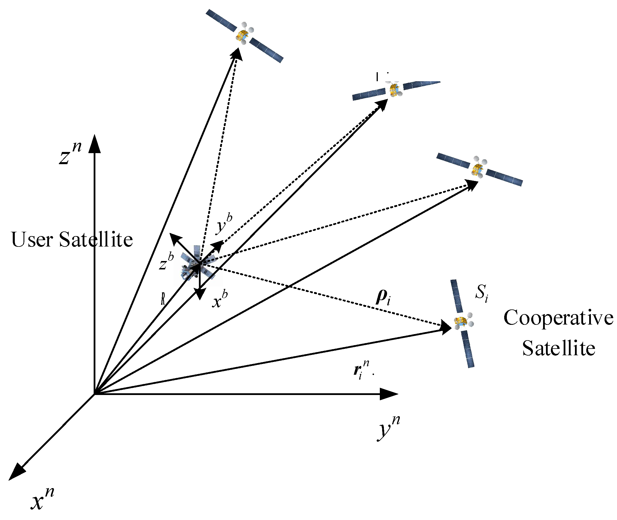
4.2. Observation Model Based on the Camera Imaging Model

In the ECI frame, the relative position of the user satellite with respect to the cooperative satellite is shown in Figure 4.

Figure 4. Relative position vector diagram of the observation model.

The inertial position of the user satellite is denoted as $R$, and the inertial position of the i^th cooperative satellite detected by the optical sensor is denoted as $r_i{}^n$. Here, we assume that the user satellite’s body frame coincides with the optical sensor frame. The coordinate transformation matrix from the ECI frame to the user satellite body frame is denoted as $C_n^b$. In the user satellite body frame, the position of the cooperative satellite is defined as:

$$r_i^b=C_n^b{\rho }_i=C_n^b\left(r_i{}^n-R\right)$$

(16)

According to the imaging model of the optical sensor, the pixel coordinates of the i^th cooperative satellite in the two-dimensional plane of the image are defined as:

$$\left[\begin{array}{c}{u}_i\\ v_i\\ 1\end{array}\right]=\frac{1}{z_i^b}\left[\begin{array}{ccc}{f}_x& 0& c_x\\ 0& f_y& c_y\\ 0& 0& 1\end{array}\right]r_i^b\stackrel{def}{=}\frac{K{r}_i^b}{z_i^b}$$

(17)

where $[u_i, v_i]$ represents the pixel coordinates, $f_x$ and $f_y$ denote equivalent focal lengths of the navigation camera, $[c_x,c_y]$ is the translation vector from the origin of the image coordinate frame to the origin of the pixel coordinate frame, and K denotes the intrinsic parameter matrix of the optical sensor and can be obtained through the calibration procedure.

Combining Equations (16) and (17), the observation equation for a single cooperative satellite is defined as:

$$c_i=\left[\begin{array}{c}{u}_i\\ v_i\end{array}\right]=\frac{1}{z_i^b}\left[\begin{array}{ccc}{f}_x& 0& c_x\\ 0& f_y& f_y\end{array}\right]C_n^b\left(r_i{}^n-R\right)=h\left(R,C_n^b\right)$$

(18)

Based on Equation (18), significant coupling is noted between position $R$ and attitude information $C_n^b$, and the observation equation has severe nonlinearity. As a consequence, it is difficult to solve the six-dimensional states simultaneously using Equation (18).

4.3. Linearized Observation Model Based on LoS Vectors’ Inner Products

In Equation (18), the coupling between the LEO satellite’s position and attitude makes it difficult to estimate the position separately. Considering that the angle between two vectors remains invariant through coordinate frame transformation, and the angle between the LEO satellite observation vectors only depends on the LEO satellite’s position and has no dependence on the LEO satellite’s attitude, the LEO satellite observation vectors’ inner product, instead of pixel coordinate measurements, is used here as the new observation, which can decouple the LEO satellite’s position and attitude.

According to Equation (17), the normalized vector ${\mathit{l}}_i$ of the cooperative satellite’s position in the LEO satellite body frame is defined as:

$${\mathit{l}}_i={\left[\begin{array}{ccc}\raisebox{1ex}{$x_i^b$}\!\left/ \!\raisebox{-1ex}{$z_i^b$}\right.& \raisebox{1ex}{$y_i^b$}\!\left/ \!\raisebox{-1ex}{$z_i^b$}\right.& 1\end{array}\right]}^T={\left[\begin{array}{ccc}{f}_x& 0& c_x\\ 0& f_y& c_y\\ 0& 0& 1\end{array}\right]}^{-1}\left[\begin{array}{c}{u}_i\\ v_i\\ 1\end{array}\right]$$

(19)

where $x_i^b,y_i^b,z_i^b$ are the three components of vector $r_i^b$ on the three axes. Through Equation (16), we obtain:

$${\mathit{l}}_i=\frac{1}{z_i^b}{\left(C_b^n\right)}^T\left(r_i{}^n-R\right)$$

(20)

Next, we denote the inner product between the i^th and j^th normalized vectors as $s_{i,j}$, and the new observation equation can be described as:

$$s_{i,j}=\frac{l_i}{\left|l_i\right|}\cdot \frac{l_j}{\left|l_j\right|}=\frac{{\left(C_b^n\right)}^T\left(r_i{}^n-R\right)}{\left|{\left(C_b^n\right)}^T\left(r_i{}^n-R\right)\right|}\cdot \frac{{\left(C_b^n\right)}^T\left(r_j{}^n-R\right)}{\left|{\left(C_b^n\right)}^T\left(r_j{}^n-R\right)\right|}$$

(21)

Since the coordinate transformation does not change the included angle between the two vectors, Equation (21) can be simplified as:

$$s_{i,j}=\frac{(r_i{}^n-R)}{\left|r_i{}^n-R\right|}\cdot \frac{(r_j{}^n-R)}{\left|r_j{}^n-R\right|}$$

(22)

We next denote the number of visible cooperative satellites as m. Then, the stacked observation matrix can be expressed as:

$$s={\left[\begin{array}{c}{s}_{1,2}\\ s_{1,3}\\ ⋮\\ s_{\left(m-1\right),m}\end{array}\right]}_{\frac{m\left(m-1\right)}{2}\times 1}$$

(23)

As shown in Equation (22), the new observation equation is only related to the position of the LEO satellite and the cooperative satellite, and the unknown states are only the LEO satellite’s position vector $R$. Therefore, the equation requires at least three inner products of LoS vectors to solve a unique solution, which means that at least three cooperative satellites should be in the field of view at the same time.

The Jacobian matrix of the observation equation is calculated as:

$$h_{i,j}={\left[\begin{array}{c}\frac{1}{AB}\left[(2x-x_i^n-x_j^n)M-\frac{N}{2M}\left((2x-2x_i^n)B+(2x-2x_j^n)A\right)\right]\\ \frac{1}{AB}\left[(2y-y_i^n-y_j^n)M-\frac{N}{2M}\left((2y-2y_i^n)B+(2y-2y_j^n)A\right)\right]\\ \frac{1}{AB}\left[(2z-z_i^n-z_j^n)M-\frac{N}{2M}\left((2z-2z_i^n)B+(2z-2z_j^n)A\right)\right]\end{array}\right]}^T$$

(24)

with

$$\begin{array}{l}M=\sqrt{{(x-x_i^n)}^2+(y-y_i^n{)}^2+(z-z_i^n{)}^2}\cdot \sqrt{{(x-x_j^n)}^2+(y-y_j^n{)}^2+(z-z_j^n{)}^2}\\ N=(x-x_i^n)(x-x_j^n)+(y-y_i^n)(y-y_j^n)+(z-z_i^n)(z-z_j^n)\\ A={(x-x_i^n)}^2+(y-y_i^n{)}^2+(z-z_i^n{)}^2\\ B={(x-x_j^n)}^2+(y-y_j^n{)}^2+(z-z_j^n{)}^2\end{array}$$

where $x_i^n,y_i^n,$ and $z_i^n$ are the three components of vector $r_i^n$; and $x,y,$ and $z$ are the three components of vector $R$. The linearization of Equation (22) can be expressed as:

$$\delta s_{i,j}=h_{i,j}\delta R$$

(25)

The stacked observation perturbation can be expressed as:

$$\delta s={\left[\begin{array}{c}\delta s_{1,2}\\ \delta s_{1,3}\\ ⋮\\ \delta s_{\left(m-1\right),m}\end{array}\right]}_{\frac{m\left(m-1\right)}{2}\times 1}$$

(26)

The corresponding stacked Jacobian matrix is expressed as:

$$H={\left[\begin{array}{c}{h}_{1,2}\\ h_{1,3}\\ ⋮\\ h_{\left(m-1\right),m}\end{array}\right]}_{\frac{m\left(m-1\right)}{2}\times 3}$$

(27)

4.4. Position Accuracy Analysis Based on the Dilution of Precision

The geometry of visible cooperative satellites is an important factor for accurate single-point positioning. The geometry changes over time due to the relative motion of the LEO with respect to cooperative satellites. The value of the dilution of precision (DOP) reflects the observability of the navigation system [17]. In this section, the DOP is introduced to evaluate position accuracy.

According to the linearized observation model in Equation (25), the weight coefficient matrix of the stacked measurement vector can be calculated as follows:

$$Q_z={(H^{T}H)}^{-1}=\left[\begin{array}{ccc}{q}_{xx}& q_{xy}& q_{xz}\\ q_{yx}& q_{yy}& q_{yz}\\ q_{zx}& q_{zy}& q_{zz}\end{array}\right]$$

(28)

If each measurement noise is mutually independent and has the same variance of ${\sigma }_0^2$, the position accuracy is calculated as:

$$m_{3D}={\sigma }_0\cdot PDOP={\sigma }_0\sqrt{\left(q_{xx}+q_{yy}+q_{zz}\right)}$$

(29)

where $m_{3D}$ is the three-dimensional (3D) position accuracy, and PDOP is a function of the principal diagonal elements of the matrix $Q_z$. Therefore, the position accuracy in different directions can be calculated as:

$$\begin{array}{l}{m}_x={\sigma }_0\cdot XDOP={\sigma }_0\sqrt{q_{xx}}\\ m_y={\sigma }_0\cdot YDOP={\sigma }_0\sqrt{q_{yy}}\\ m_z={\sigma }_0\cdot ZDOP={\sigma }_0\sqrt{q_{zz}}\end{array}$$

(30)

where $m_x, m_y,$ and $m_z$ are the X-axis, Y-axis, and Z-axis position accuracies, respectively, and the XDOP, YDOP, and ZDOP are the position dilution of precision in the X-axis, Y-axis, and Z-axis, respectively.

5. Navigation Algorithm Design

5.1. Single-Point Positioning Algorithm

The principle of least-squares batch filtering is to determine a set of states that minimize the sum of the squares of the measurement residuals. For the nonlinear observation Equation (22), the ILS batch filter iteratively improves state estimation using the first-order partial derivatives of the linearized system [23]. In this section, an ILS filter is introduced to estimate the LEO satellite’s position.

The process of the single-point positioning algorithm is described in Algorithm 1.

Algorithm 1. Single-point positioning algorithm.

Input: A series of pixel measurement ${\left\{c_i\right\}}_{i=1,2,\dots m}$, ephemeris of visible cooperative Satellites ${\left\{r_i{}^n\right\}}_{i=1,2,\dots ,m}$, and initial state $R^{(0)}$

Output: Position vector of user satellite $R$ and its covariance matrix $P$

1: Initialize the corrected position with $\Delta R^{(k)}=1$ and initialize the iteration order with $k=0$

2: for $i=1,2\dots ,m$ do

3: $l_i\leftarrow \mathrm{Equation} (20)$

4: end for

5: Generate the new real measurement $s_i$ using Equations (22) and (23)

6: If $|\Delta R^{(k)}|\ge {10}^{-3}$ then

7: for $n=1,2,\dots ,m-1$ do

8:  for $j=n+1,\dots ,m$ do

9:     $s_{n,j}\leftarrow \mathrm{Equation} (22)$

10:   end for

11: end for

12: ${\widehat{s}}^{(k)}\leftarrow \mathrm{Equation} (23)$

13: The measurement deviation $Y^{(k)}={\widehat{s}}^{(k)}-s$

14: Calculate the Jacobian matrix $H^{(k)}$ using Equations (24) and (27)

15: Calculate the corrected position $\Delta R^{(k)}$ with $\Delta R^{(k)}={({(H^{(k)})}^T)}^{-1}{(H^{(k)})}^T{Y}^{(k)}$

16: $R^{(k+1)}=R^{(k)}-\Delta R^{(k)}$

17: $k=k+1$

18: Else

19: Calculate the covariance matrix $P$ with $P={\sigma }_0^2{(H^{{(k)}^T}{H}^{(k)})}^{-1}$

20: $R=R^{(k)}$

21: Output the final estimated position $R$ and its covariance matrix $P$

22: end if

5.2. Batch Dynamic Orbit Determination Algorithm

Due to the errors in the measured pixel coordinates, there are also large errors in the single-point positioning results. When the pixel coordinate measurement errors are very large or the LEO satellite is far from the cooperative satellites, the accuracy of single-point positioning may be unsatisfactory. Thus, batch dynamic orbit determination is introduced to further improve navigation accuracy.

First, the positions of the LEO satellite estimated from single-point positioning are arranged according to their time sequences. The velocity of the LEO satellite in each epoch can be obtained using the third-order polynomial fitting of the position sequences. Then, we can obtain a series of positions and velocities as:

$$[R(1);V(1)],[R(2);V(2)],\cdots ,[R(t_n);V(t_n)]$$

(31)

Next, we denote the estimated position and velocity at time t as $x_t$ and obtain:

$$x_t=[R(t);V(t)]$$

(32)

We then take the estimated position $R(t)$ as the observation and the estimated position and velocity at the initial time as the state. The resulting observation equation can be described as:

$$R(t)=\left[\begin{array}{cc}{I}_{3\times 3}& {\mathsf{0}}_{3\times 3}\end{array}\right]f(x_0,t)$$

(33)

where $f(,)$ represents the orbit integrator, which depends on the dynamic model.

The observation $R(t)$ is obtained from the single-point positioning algorithm, thus containing errors and the covariance matrix of $P$.

The linearized perturbation of Equation (33) is obtained as:

$$\delta R(t)=\left[\begin{array}{cc}{I}_{3\times 3}& {\mathsf{0}}_{3\times 3}\end{array}\right]\Phi \left(t,t_0\right)\delta x_0=h(t)\delta x_0$$

(34)

where $\Phi \left(t,t_0\right)$ denotes the state transmission matrix from $t_0$ to $t$, and $h(t)$ represents the partial derivative matrix of $R(t)$ with respect to $x_0$.

We next assume that there are k epochs in a time sequence: stacked linearized observations, the stacked Jacobian matrix, and the stacked covariance matrix of the observation noise can be expressed using Equations (35)–(37), respectively:

$$Z={[\begin{array}{cccc}\delta R(1)& \delta R(2)& \cdots & \delta R(t_n)\end{array}]}^T$$

(35)

$$H={[\begin{array}{cccc}h(1)& h(2)& \cdots & h(t_n)\end{array}]}^T$$

(36)

$$C_W={\left[\begin{array}{cccc}{P}_1& 0& 0& 0\\ 0& P_2& 0& 0\\ 0& 0& \ddots & 0\\ 0& 0& 0& P_k\end{array}\right]}_{3t_n\times 3t_n}$$

(37)

The process for the batch dynamic orbit determination algorithm is described in Algorithm 2.

Algorithm 2. Batch dynamic orbit determination algorithm.

Input: A time series of position vectors $R_{series}$ and covariance matrix ${\left\{P_t\right\}}_{t=1,2,\dots ,t_n}$ obtained from Algorithm 1 Output: Initial orbital state ${\tilde{x}}_0$

1: Generate a series of positions and velocities with Equation (31) using third-order polynomial fitting

2: Set initial state $x_0=[R(1);V(1)]$. Initialize the state correction with $\Delta x^{(k)}=1$ and initialize the iteration order with $k=0$

3: Calculate the stacked covariance matrix of observation noise $C_W$ using Equation (37)

4: If $|\Delta x^{(k)}|\ge {10}^{-3}$ then

5: Generate a predicted position sequence ${\tilde{R}}_{series}^{\left(k\right)}$ using the orbital integrator 6: ${\tilde{R}}_{series}^{\left(k\right)}\leftarrow {\left[\begin{array}{cccc}\tilde{R}(1)& \tilde{R}(2)& \cdots & \tilde{R}(t_n)\end{array}\right]}^T$

7: Generate a series for the state transition matrix ${\left\{\Phi {(t,t_0)}^{(k)}\right\}}_{t=1,2,\dots t_n}$

8: $Z^{(k)}={\tilde{R}}_{series}^{(k)}-R_{series}$

9: Calculate the Jacobian matrix $H$ using Equations (34) and (36)

10: Calculate the corrected position $\Delta x^{(k)}\leftarrow {(H^T{C}_W{}^{-1}H)}^{-1}{H}^T{C}_W{}^{-1}{Z}^{(k)}$

11: $x_0^{(k+1)}=x_0^{(k)}-\Delta x_{}^{\left(k\right)}$

12: $k=k+1$

13: Else

14: ${\tilde{x}}_0=x_0^{(k)}$

15: Output the estimated initial orbital state ${\tilde{x}}_0$

16: end if

6. Simulation and Results

In this study, numerical simulations are conducted to verify the feasibility and performance of the proposed cooperative constellation navigation system. In addition, several factors that could influence the performance of the navigation system are examined, including the noise levels of measurements, critical parameters of cooperative constellations, cooperative satellite ephemeris errors, and the truncated degree and order of the Earth’s gravitational model in the ILS process.

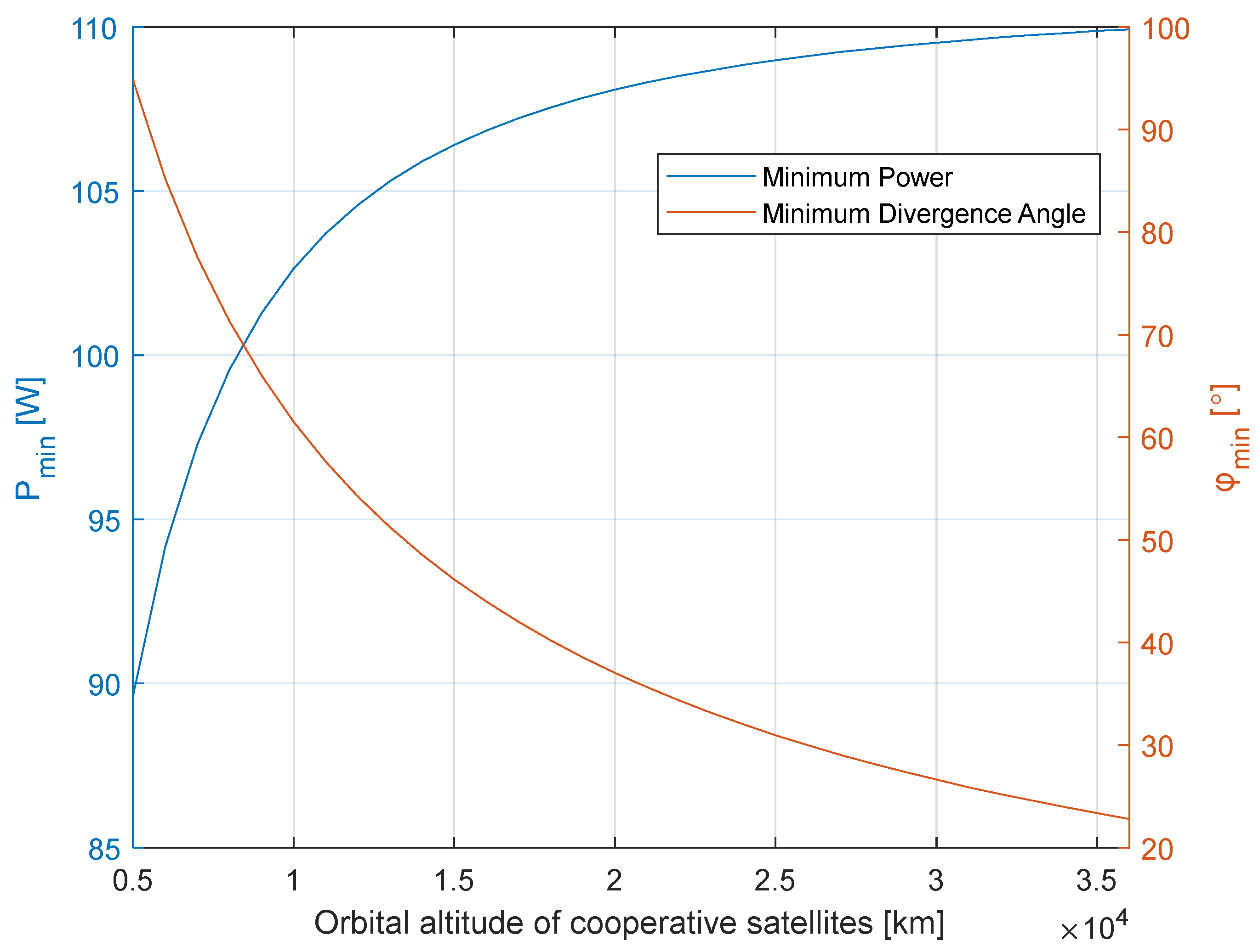
6.1. Optical Link Budget

In order to verify the feasibility of the CCNS, it is necessary to calculate the power demand and divergence angle of the light source onboard cooperative satellites at different orbital altitudes. An optical sensor array with a wide FOV is used in the CCNS. Table 2 shows the parameters of the optical sensor onboard the LEO satellite. In addition, in order to test the power demand in extreme cases, the radiation angle $\theta$ is set to $\phi /2$, the incident angle $\alpha$ is set to 15°, and the SNR is set to 5. The orbital altitude of the cooperative constellations varies from 5000 to 36000 km.

Table 2. Optical sensor parameters.

Parameters	Value
Aperture, m	0.2
FOV of sensor array, °	150
FOV of single sensor	30
Spectral transmittance	0.56
Array size, pixel	1024 × 1024
Fill factor pixel	0.44
Quantum efficiency	0.66
Integration period, s	0.02
Dark current noise, e-/pixel-second	3.5
Readout noise, e-	6

Figure 5 shows the minimum values of the divergence angle with the optical signal constraints in Equation (2) and the minimum power of the light source with SNR constraints in Equation (13) given different orbital altitudes of cooperative satellites. As expected, the light source of the smaller divergence angle is required with an increase in the orbital altitude of cooperative satellites, which reduces signal energy divergence. However, an increase in the orbital altitude of cooperative satellites produces more signal energy diffusion. Under the combined effects, the light source power demand varies little with the orbital altitude. For a cooperative satellite with an orbital altitude of 36,000 km, the power demand of the light source reaches 110 w, and the divergence angle is about 23°. For a cooperative satellite with an orbital altitude of 5000 km, the power demand of the light source reaches 89 w, and the divergence angle is about 108°.

Figure 5. Minimum divergence angle and power of the light source (SNR = 5).

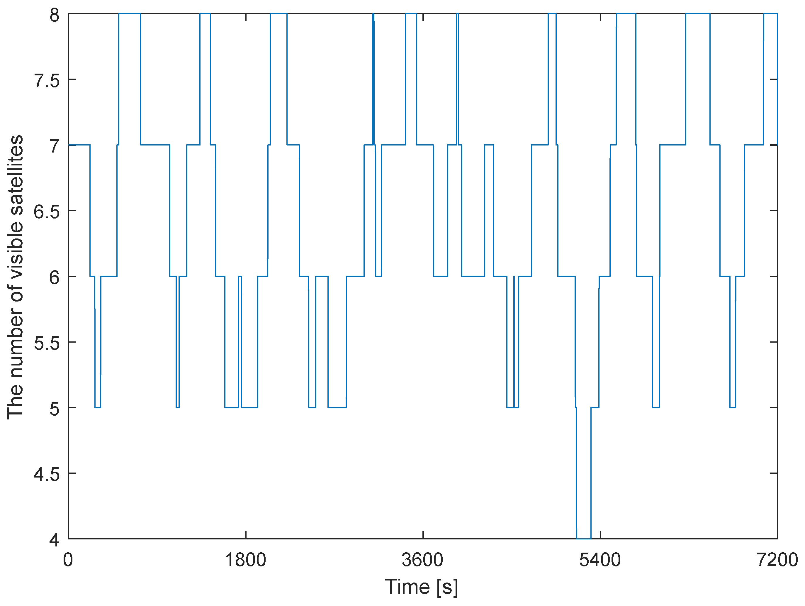
6.2. Navigation Simulation Scenario

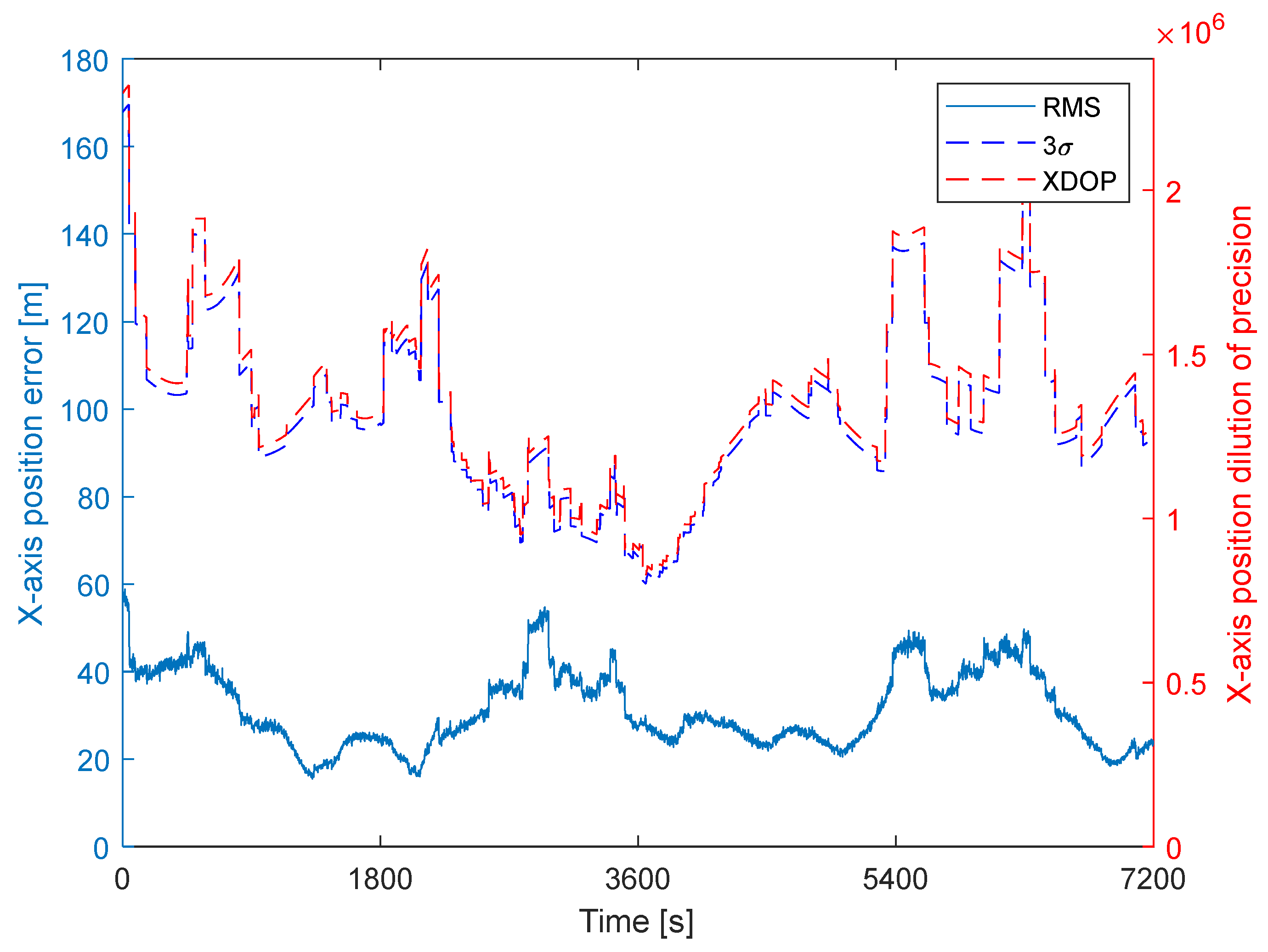
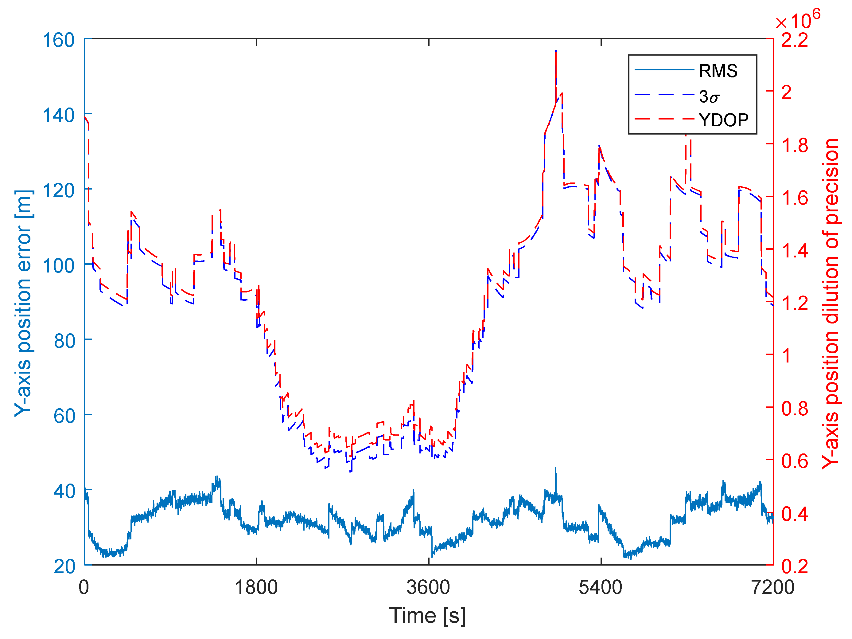
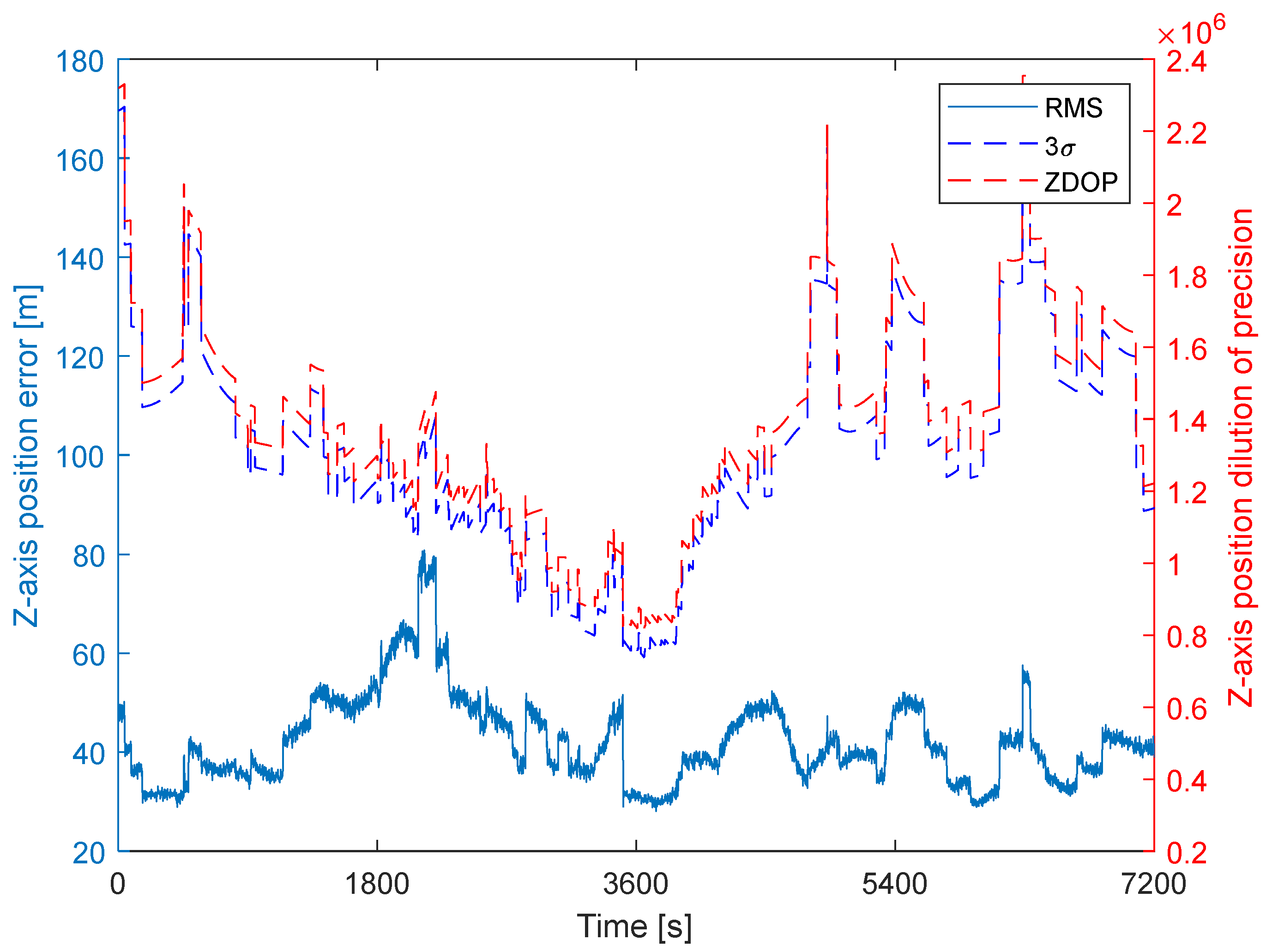
In order to verify the performance of the CCNS, the LEO satellite is assumed to move along a nearly circular orbit with a 500 km height, and the Walker constellation is selected as the cooperative satellite constellation. In this simulation scenario, the total number of satellites of the cooperative constellation is 54, the number of orbital planes is 6, and the configuration number is set to 1. Table 3 shows the specific parameters of the simulation scenario. The true orbit trajectories are generated using a high-precision numerical orbit simulator. In the simulator, we use Earth’s gravitational model (2008) truncated at degree 70 and order 70 for gravitational acceleration, the NRLMSISE-00 model for atmospheric density, and the analytical formulas for lunar and solar ephemerides. The simulation covers a 2 h data arc starting from February 21, 2022, at 00:00:00.0 (UTC). Moreover, in order to examine the performance in a probabilistic manner, a 500 run Monte Carlo simulation is performed for each single-point positioning process.

Table 3. Simulation scenario parameters.

Parameters		Value
LEO satellite	Semi-major axis, km	6878.14
	Eccentricity	0.00074
	Inclination, °	30
	Right ascension of ascending node, °	210.1
	Argument of perigee, °	8.2
	Mean anomaly, °	215.8
Cooperative constellation	Inclination, °	55
	Satellite number	54
	Orbital plane number	6
	Constellation configuration number	1

6.3. Baseline Case

For the baseline case, the orbital altitude of the cooperative constellation is assumed to be 5000 km. The optical sensor noise is assumed to be Gaussian white with a standard deviation of 5 arcsecs. The ephemeris errors of the cooperative constellation are set to 10 m, and the observation sampling interval is set to 1 s.

Figure 6 shows the evolution of the number of visible cooperative satellites over time. To test the navigation performance of the cooperative constellation navigation system, the results of single-point positioning and orbit determination are examined. Figure 7, Figure 8 and Figure 9 show the evolutions of single-point positioning errors and DOPs over time. Table 4 shows the root mean square (RMS) of the position errors. It can be seen that variations in the 3-sigma values of the position errors and the values of the DOP are consistent, which demonstrates that the DOP can effectively reflect the position accuracy.

Figure 6. The number of visible cooperative satellites.

Figure 7. RMS of the X-axis position error and the corresponding 3-sigma and XDOP values.

Figure 8. RMS of the Y-axis position error and the corresponding 3-sigma and YDOP values.

Figure 9. RMS of the Z-axis position error and the corresponding 3-sigma and ZDOP values.

Table 4. RMS of position errors of single-point positioning and orbit determination.

Direction	RMS of Position Errors, m
	Single-Point Positioning	Dynamic Orbit Determination (The Degree and Order of the Earth’s Gravitational Model)
		8 × 8	20 × 20	60 × 60
3D	63.40	19.7616	8.0532	2.0006
X-axis	32.90	4.7296	3.5525	1.4577
Y-axis	32.49	19.0814	6.4748	0.7508
Z-axis	43.38	13.6106	3.2110	1.1462

Figure 10 shows the initial position errors of dynamic orbit determination with Earth’s gravitational models truncated at different degrees. Here, the initial position accuracies of the dynamic orbit determination are greatly improved by 43~60 m compared to those of the single-point positioning. In addition, by increasing the truncated degree of Earth’s gravitational model, the position error gradually decreases.

Figure 10. 500 Monte Carlo simulations of the initial position error of dynamic orbit determination: (a) top, with a truncated degree and order of 8 × 8; (b) middle, with a truncated degree and order of 20 × 20; (c) bottom, with a truncated degree and order of 60 × 60.

6.4. Influence Factor Analysis

In order to investigate the factors that influence navigation accuracy, the parameters for the noise level of optical measurements, critical parameters of cooperative constellation, truncated degree of the Earth’s gravitational model, and cooperative satellites’ ephemeris errors are changed. Numerical simulations are then performed to analyze the influence of these parameters on navigation accuracy.

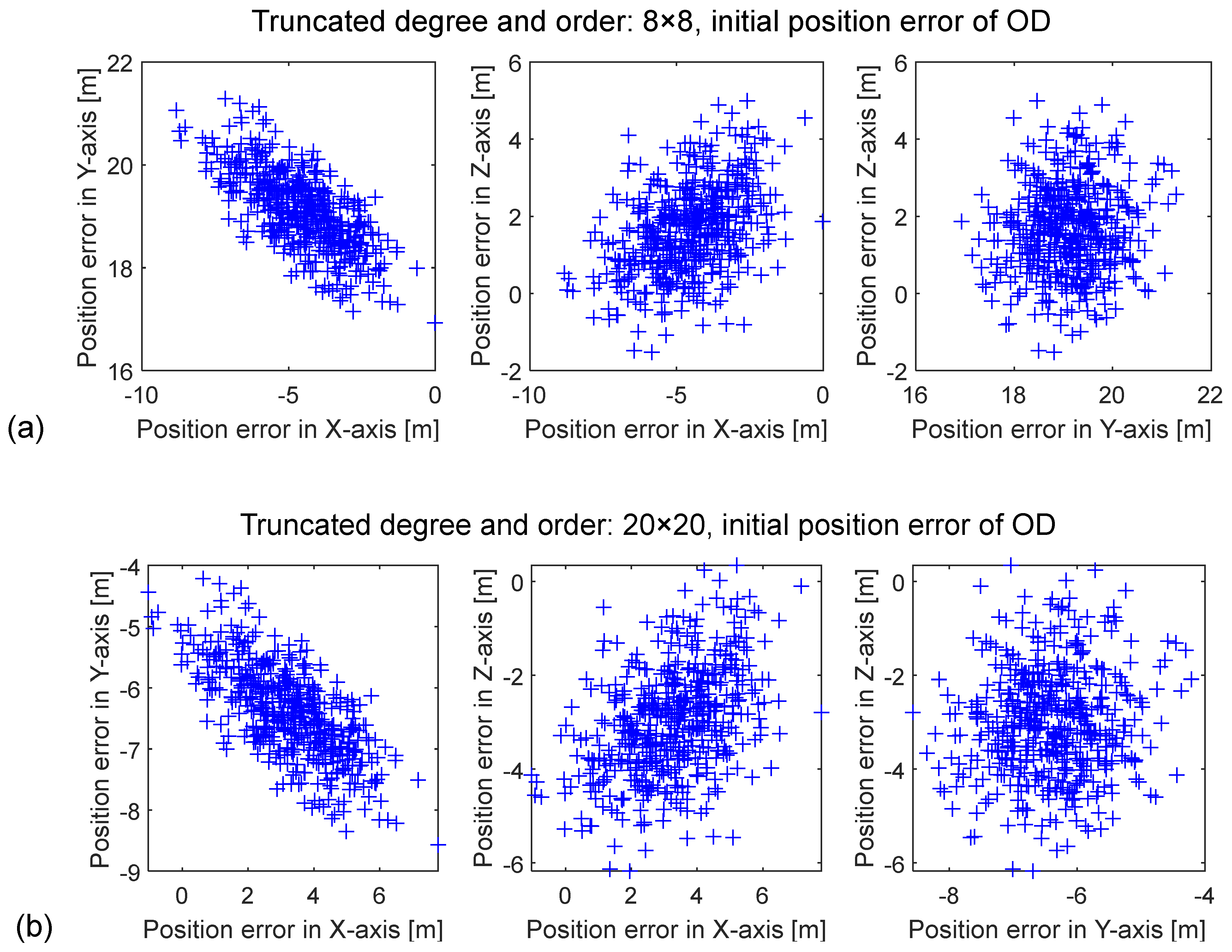
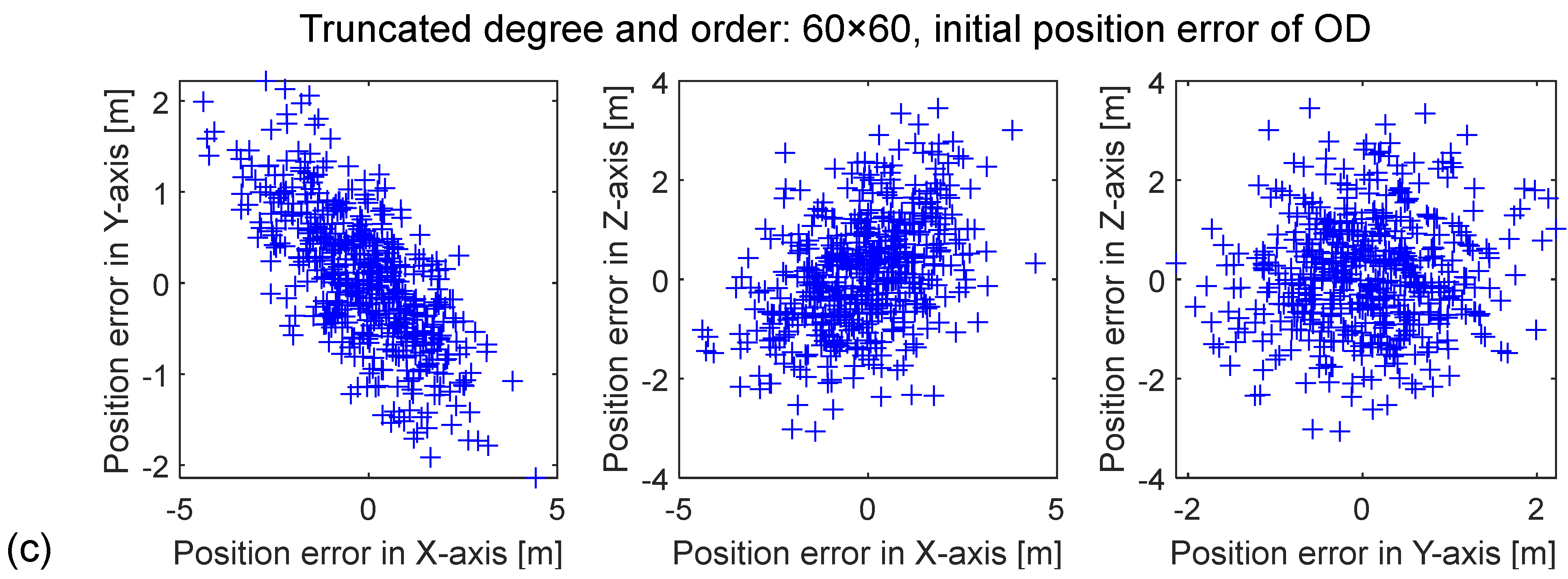
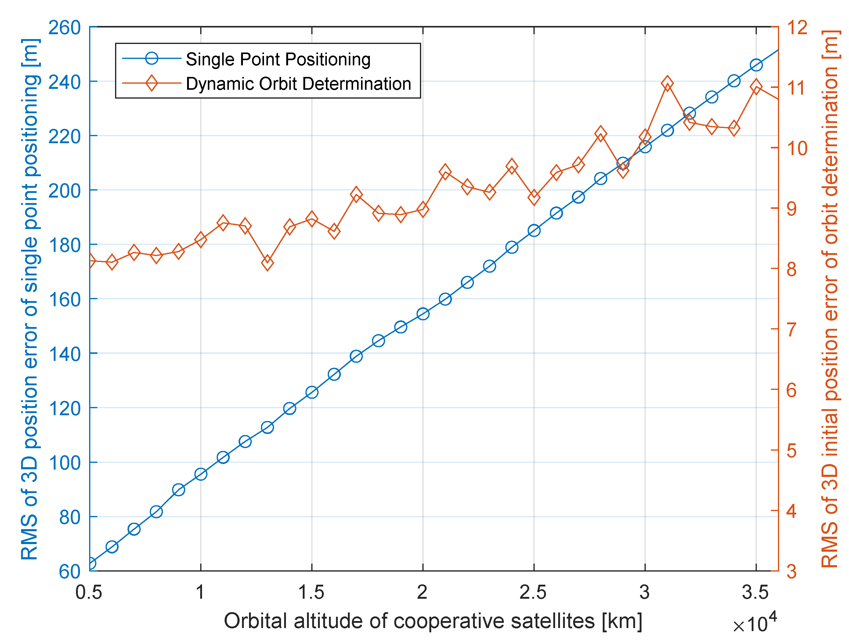
6.4.1. Cooperative Constellation Parameters

First, the effects of the orbital altitude of the cooperative constellations are investigated. The distances between the LEO satellite and cooperative satellites, as well as the observations in Equation (24), depend on the orbital altitude of the cooperative constellations, which is a key parameter in navigation. Cases with different cooperative constellation orbital altitudes from 5000 to 36,000 km are simulated. The truncated degree and order of the Earth’s gravitational model is set to 20×20. The rest of the simulation conditions are the same as those of the baseline case.

The statistical RMS values of the 3D position errors are shown in Figure 11. Here, an increase in the orbital altitude of cooperative constellation results in low navigation accuracy. By increasing the orbital altitude of the cooperative constellation, the number of visible cooperative satellites increases, which slightly improves the DOP. The distances between the LEO satellite and cooperative satellites also increase, which results in the serious deterioration of the DOP. Under the combined effects, the navigation accuracy of single-point positioning significantly degrades. After adopting dynamic orbit determination, navigation accuracy is greatly improved. In addition, the influence of orbital altitude on the navigation errors of orbital determination becomes smaller than that on the position errors of single-point positioning.

Figure 11. RMS of the 3D position errors of different orbital altitudes of cooperative satellites.

The effects of the number of cooperative satellites are also examined, and different numbers of cooperative satellites from 54 to 90 are adopted. In this simulation, the truncated degree and order of the Earth’s gravitational model is set to 20×20. The rest of the simulation conditions are the same as those of the baseline case. The statistical RMS values of the 3D position errors for these cases are shown in Figure 12. As the number of cooperative satellites increases, more abundant observation geometry can be obtained, leading to better positioning accuracy.

Figure 12. RMS of 3D position errors of different cooperative satellite numbers.

Next, the effects of the orbital plane number and constellation configuration number are investigated. The orbital plane number is set to three different values of 3, 6, and 9. The truncated degree and order of the Earth’s gravitational model is set to 20×20. The statistical RMS of the 3D position errors with different orbital plane numbers is shown in Table 5. The position accuracy increases slowly with an increase in the orbital plane number. This phenomenon occurs because as the orbital plane number increases, the observed cooperative satellite number slightly improves.

Table 5. RMS of 3D position errors of different orbital plane numbers.

Orbital Plane Number	RMS of 3D Position Errors, m
	Single-Point Positioning	Dynamic Orbit Determination
3	74.33	8.2460
6	63.40	8.0532
9	58.58	7.9018

Finally, the effects of the constellation configuration number are also analyzed. The different constellation configuration numbers are set to 1, 1.5, and 2. The truncated degree and order of the Earth’s gravitational model are set to 20×20. The statistical RMS of the 3D position errors of the different constellation configuration numbers are shown in Table 6. It can be seen that the constellation configuration number has little effect on navigation accuracy.

Table 6. RMS of the 3D position errors of different constellation configuration numbers.

Constellation Configuration Number	RMS of 3D Position Errors, m
	Single-Point Positioning	Dynamic Orbit Determination
1	63.40	8.0532
1.5	65.79	8.0263
2	64.52	7.8947

6.4.2. Ephemeris Errors of Cooperative Satellites

The ephemeris errors are set to four different values: 0, 10, 50, and 100 m. The truncated degree and order of the Earth’s gravitational model are set to 20×20. The remainder of the simulation conditions remain the same as those of the baseline case.

The statistical RMS values of 3D position errors for these cases are shown in Table 7. As the ephemeris errors increase, the single-point positioning errors also increase greatly, whereas the position errors of dynamic orbit determination increase slightly. When the cooperative satellite orbit determination accuracy is at a 100 m level, the ephemeris errors of cooperative satellites have little effect on navigation accuracy.

Table 7. RMS of the 3D position errors of different Ephemeris errors.

Ephemeris Errors of Cooperative Satellites, m	RMS of 3D Position Errors, m
	Single-Point Positioning	Dynamic Orbit Determination
0	62.80	8.0472
10	63.40	8.0532
50	75.65	8.1918
100	105.21	8.6188

6.4.3. Noise Level of Measurement

Here, the noise level of optical measurements is set to three different values: 5 arcsecs, 10 arcsecs, and 15 arcsecs. The truncated degree and order of the Earth’s gravitational model is set to 20×20. The rest of the simulation conditions are the same as the baseline case.

The statistical RMS 3D position errors for these cases are shown in Table 8. Here, navigation accuracy is approximately linear to the noise level of optical measurements. In addition, by increasing the noise level of the optical measurements, navigation accuracy is greatly reduced. As a consequence, the optical measurement noise level is taken as the main parameter affecting navigation accuracy.

Table 8. RMS of 3D position errors of different measurement noise levels.

Measurement Noise, Arcsec	RMS of 3D Position Errors, m
	Single-Point Positioning	Dynamic Orbit Determination
5	63.40	8.0532
10	125.76	9.5117
15	188.39	11.0676

According to the above simulation results and analysis, the proposed cooperative constellation navigation system along with the related single-point positioning and batch orbit determination algorithm can effectively navigate the LEO satellite. The simulation results can be summarized as follows:

(1)

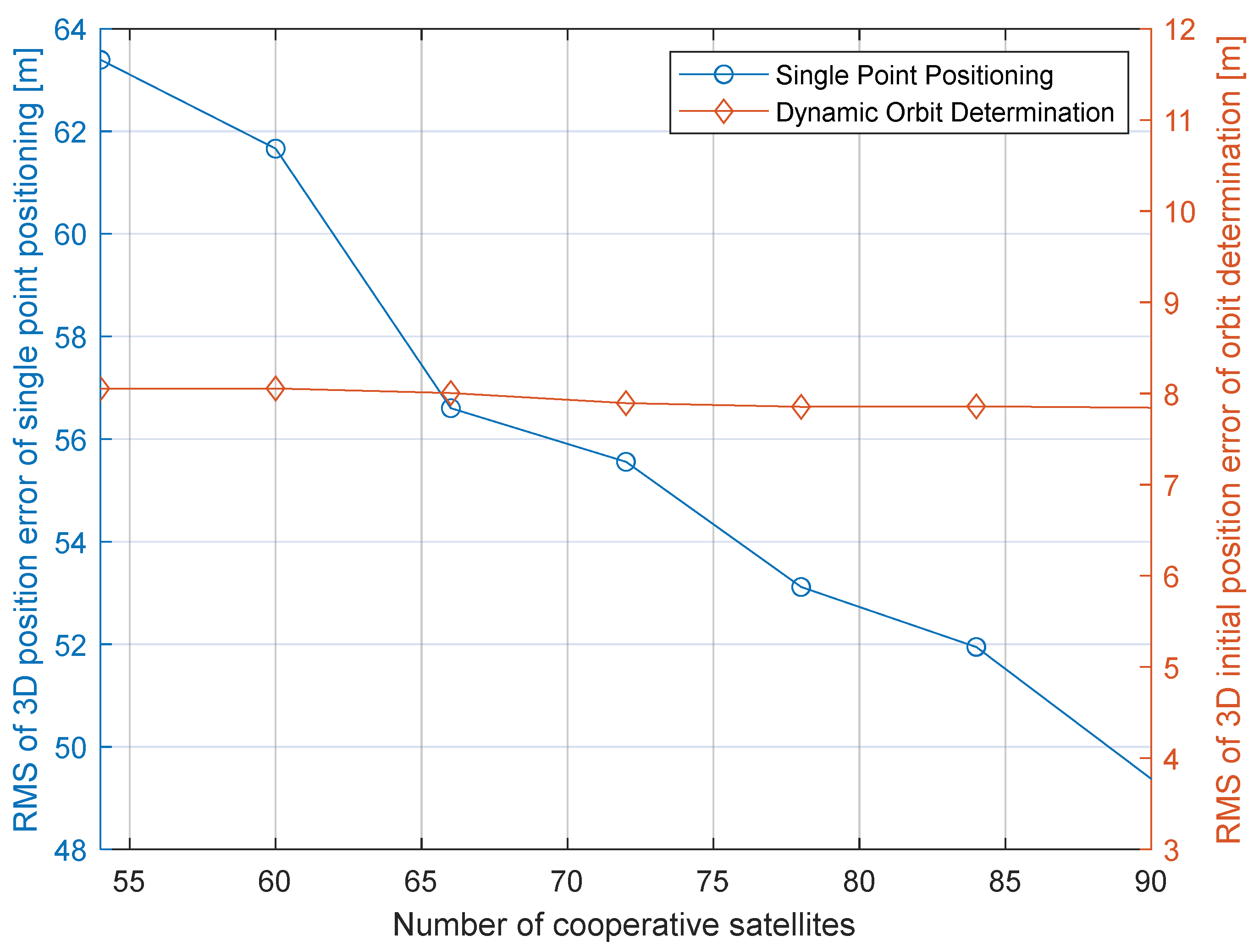
For critical parameters of cooperative constellations, reducing the orbital altitude of cooperative satellites and increasing the number of cooperative satellites can improve navigation accuracy. The position accuracy increases slowly with an increase in the orbital plane number, and the constellation configuration number has little effect on navigation accuracy.

(2)

The ephemeris error of the cooperative satellite has little influence on navigation accuracy.

(3)

The optical measurement error is the main factor that affects navigation accuracy. Thus, it is vital to carry a dedicated optical sensor onboard the LEO satellite to realize accurate navigation.

(4)

After introducing the dynamic orbit determination method, the navigation accuracy of the navigation system is greatly improved, and the influence of external factors on navigation accuracy is greatly reduced.

(5)

The influence of Earth’s gravitational model errors on navigation accuracy is evident, as Earth’s gravitational model errors can significantly affect orbit propagation errors. Therefore, reducing dynamic model errors is of great importance in realizing high-precision orbit determination.

7. Conclusions

In this paper, we propose a new navigation method for LEO satellites based on optical measurement of a cooperative constellation and built an optical transmission link model. Additionally, simulations of the power demand and divergence angle of the light source of cooperative satellites at different orbital altitudes are developed to verify the feasibility of the CCNS. Because directly determining the LEO satellite’s position with optical pixel coordinate observations is complicated, the inner product of the line-of-sight vector is introduced as a new measurement to decouple the position and attitude state. Then, the least square method is employed to realize single-point positioning. Furthermore, in order to improve single-point positioning accuracy, batch orbit determination with ILS is developed. For a case with an ephemeris error of 10 m and measurement noise levels of 5 arcsecs, a navigation accuracy of 8.05 m (3D) is observed. In addition, the influences of the critical parameters of cooperative constellation, ephemeris error, noise level of optical measurements, and truncated degree of the Earth’s gravitational model on navigation accuracy are investigated using comparative simulations.

References

1. Oliver, M.; Eberhard, G. Satellite Orbits; Springer: Berlin/Heidelberg, Germany; New York, NY, USA, 2000. [Google Scholar]
2. ESA Space Debris Office. ESA’S Annual Space Environment Report, 2022; ESA: Paris, France, 2022. [Google Scholar]
3. Montenbruck, O.; van Helleputte, T.; Kroes, R.; Gill, E. Reduced dynamic orbit determination using GPS code and carrier measurements. Aerosp. Sci. Technol. 2005, 9, 261–271. [Google Scholar] [CrossRef]
4. Bock, H.; Jaggi, A.; Meyer, U.; Visser, P.; van den IJssel, J.; van Helleputte, T.; Heinze, M.; Hugentobler, U. GPS-derived orbits for the GOCE satellite. J. Geodesy 2011, 85, 807–818. [Google Scholar] [CrossRef]
5. Tippenhauer, N.O.; Popper, C.; Rasmussen, K.B.; Capkun, S. On the requirements for successful GPS spoofing attacks. In Proceedings of the ACM Conference on Computer & Communications Security, Chicago, IL, USA, 17–21 October 2011; p. 75. [Google Scholar]
6. Ning, X.L.; Fang, J.C. An autonomous celestial navigation method for LEO satellite based on unscented Kalman filter and information fusion. Aerosp. Sci. Technol. 2007, 11, 222–228. [Google Scholar] [CrossRef]
7. Ning, X.L.; Wang, L.H.; Bai, X.B.; Fang, J.C. Autonomous satellite navigation using starlight refraction angle measurements. Adv. Space Res. 2013, 51, 1761–1772. [Google Scholar] [CrossRef]
8. Qian, H.M.; Sun, L.; Cai, J.N.; Huang, W. A starlight refraction scheme with single star sensor used in autonomous satellite navigation system. Acta Astronaut. 2014, 96, 45–52. [Google Scholar] [CrossRef]
9. Xu, C.; Wang, D.Y.; Huang, X.Y. Landmark-based autonomous navigation for pinpoint planetary landing. Adv. Space Res. 2016, 58, 2313–2327. [Google Scholar] [CrossRef]
10. Zhu, S.Y.; Liu, D.C.; Liu, Y.; Cui, P.Y. Observability-based visual navigation using landmarks measuring angle for pinpoint landing. Acta Astronaut. 2018, 155, 313–324. [Google Scholar] [CrossRef]
11. Ogawa, N.; Terui, F.; Yasuda, S.; Matsushima, K. Image-based Autonomous Navigation of Hayabusa2 using Artificial Landmarks: Design and In-Flight Results in Landing Operations on Asteroid Ryugu. In Proceedings of the AIAA Scitech 2020 Forum, Orlando, FL, USA, 6–10 January 2020. [Google Scholar] [CrossRef]
12. Psiaki, M.L. Absolute Orbit and Gravity Determination Using Relative Position Measurements Between Two Satellites. J. Guid. Control Dyn. 2011, 34, 1285–1297. [Google Scholar] [CrossRef]
13. Luo, Y.; Qin, T.; Zhou, X.Y. Observability Analysis and Improvement Approach for Cooperative Optical Orbit Determination. Aerospace 2022, 9, 166. [Google Scholar] [CrossRef]
14. Huang, J.; Lei, X.; Zhao, G.; Liu, L.; Li, Z.; Luo, H.; Sang, J. Short-Arc Association and Orbit Determination for New GEO Objects with Space-Based Optical Surveillance. Aerospace 2021, 8, 298. [Google Scholar] [CrossRef]
15. Flohrer, T.; Krag, H.; Klinkrad, H.; Schildknecht, T. Feasibility of performing space surveillance tasks with a proposed space-based optical architecture. Adv. Space Res. 2011, 47, 1029–1042. [Google Scholar] [CrossRef]
16. Hu, Y.P.; Bai, X.Z.; Chen, L.; Yan, H.T. A new approach of orbit determination for LEO satellites based on optical tracking of GEO satellites. Aerosp. Sci. Technol. 2018, 11, 222–228. [Google Scholar] [CrossRef]
17. Bernhard, H.W.; Herbert, L.; Elmar, W. GNSS—Global Navigation Satellite Systems; Springer: Vienna, Austria, 2008; pp. 309–340. [Google Scholar]
18. Luba, O.; Boyd, L.; Gower, A.; Crum, J. GPS III system operations concepts. IEEE Aerosp. Electron. Syst. Mag. 2005, 20, 10–18. [Google Scholar] [CrossRef]
19. William, L.W. Methods in Experimental Physics; Elsevier: London, UK, 1989; pp. 213–289. [Google Scholar] [CrossRef]
20. Anbarasi, K.; Hemanth, C.; Sangeetha, R.G. A review on channel models in free space optical communication systems. Opt. Laser Technol. 2017, 97, 161–171. [Google Scholar] [CrossRef]
21. Baeza, V.M.; Lagunas, E.; Al-Hraishawi, H.; Chatzinotas, S. An Overview of Channel Models for NGSO Satellites. In Proceedings of the IEEE 96th Vehicular Technology Conference, London, UK, 26–29 September 2022. [Google Scholar]
22. Engstrom, R.W. Electro-Optics Handbook; FDA: Rockville, MD, USA, 1974. [Google Scholar]
23. Bar-Shalom, Y.; Li, R.; Kirubarajan, T. Estimation with Applications to Tracking and Navigation: Theory Algorithms and Software; John Wiley & Sons: Hoboken, NJ, USA, 2001. [Google Scholar]
Disclaimer/Publisher’s Note: The statements, opinions and data contained in all publications are solely those of the individual author(s) and contributor(s) and not of MDPI and/or the editor(s). MDPI and/or the editor(s) disclaim responsibility for any injury to people or property resulting from any ideas, methods, instructions or products referred to in the content.
Article Metrics
Citations
Article Access Statistics
Multiple requests from the same IP address are counted as one view.