Numerical Simulations in Ultrasonic Guided Wave Analysis for the Design of SHM Systems—Benchmark Study Based on the Open Guided Waves Online Platform Dataset

Abstract

Structural health monitoring (SHM) strategies based on ultrasonic guided waves are very promising regarding thin-walled lightweight structures. To study the performance of such systems, validated numerical analysis tools have to be used. For that procedure, a benchmark between two numerical methods will be presented. The first promising approach is the elastodynamic finite integration technique (EFIT). Miscellaneous research shows that its capability of capturing wave characteristics and interactions is advanced in various media and structures, including thin-walled composites. The second approach employs conventional shell-type finite elements following the Reissner–Mindlin theory for modelling layered composite structures. The advantage of using such finite element methods (FEM) is their high availability in general purpose simulation tools. As a reference model, the measurement data coming from the Open Guided Waves Project (OGW) was taken into account. The OGW dataset provides the experimental data of ultrasonic guided wave propagation in carbon fiber composite plates with an additional omega stringer. By using this contribution, this experiment was reproduced by simulation. The paper presents the results of a validation and motivates further research, such as in research related to the probability of detection analysis and numerical performance.

1. Introduction

Over the last years, ultrasonic guided waves (UGW) have become a main topic of research in the field of structural health monitoring (SHM) systems [1,2,3,4]. The realization of UGW-based SHM concepts has been investigated regarding a large variety of engineering applications, e.g., aerospace and the inspection of plant constructions [5]. SHM not only may improve the safety of technical systems, but also can ultimately help to save material usage and costs. Especially considering lightweight structures, smart condition monitoring systems might contribute to decreasing environmental pollution by saving energy consumption.

Due to the great complexity of the interacting physical phenomena and technical principles, enormous efforts have to be undertaken in developing suitable concepts. Consequently, the design process and the adaption of such monitoring systems cannot only be covered by laboratory testing. Rather, this process has to be accompanied by model-assisted methods. At this point, numerical simulations offer a great potential for reducing time and saving costs.

Apart from analytical and semi-analytical methods, there exist various approaches to simulate UGW propagation numerically [6]. The finite element method has become a major simulation tool in a wide range of scientific and engineering areas [7,8,9]; it was also adapted to the ultrasonic guided wave analysis of thin-walled structures [10]. Suitable finite element concepts have to capture the characteristics of UGW processes that have very high propagation frequencies and short wavelengths. Hence, such finite element implementations are often realized as the so-called spectral element method (SEM) [11]. This method can be seen as a special form of the p-version of finite element refinement [12]. The SEM uses Lagrange polynomials for interpolation within an element and nodes defined on Gauss–Labatto-Legendre or Chebyshev–Gauss–Labatto points [13,14]. Based on this approach, different plate, shell, and 3D continuum finite elements have been developed [15]. Although there has been some progress in transferring high-order applications to particular non-destructive evaluation analysis tools [16], the main disadvantage of SEM and other advanced techniques [17] is that they are still not available in commonly used FEM simulation tools. Furthermore, additional effort arises in model data handling when existing finite element models should be transferred to special tools.

Along with growing computational resources, low-order finite shell element techniques might be an alternative choice while dealing with thin-walled lightweight structures. Consequently, these techniques have to follow the h-version of finite elements refinement [12], where the geometrical dimensions of elements are decreased in models coming, for instance, from strength or modal analysis. The derived models are actually limited to certain low-frequency ranges and can only reproduce certain Lamb wave mode phenomena. Above all, the propagation of the first anti-symmetric Lamb wave mode $A_0$, which is of great importance for damage detection in composite structures [18,19], ought to be investigated sufficiently. Thus, validated and robust numerical analysis tools must be used for model-assisted GW-based SHM studies.

Another method adapted to simulate UGW, especially for thin-walled lightweight structures, is the elasto-dynamic finite integration technique (EFIT), which was first launched as a computational tool for real-life non-destructive evaluation (NDE) implementations and general purpose wave propagation problems. It was introduced and analysed by Fellinger for electromagnetics [20,21]. The approach can be referred to as the finite volume method (FVM), and it is equivalent to the finite difference—time domain method (FDTD) approach in Cartesian coordinates; the major difference comes from the discretization procedure. EFIT uses the integral form instead of the differential form for governing equations, which leads to highly stable, convergent numerical behavior that is also suitable for high-performance vector and/or parallel computer implementations [22]. Further, the EFIT scheme shows a decent performance combination with the efficient modeling approaches of layered media such as the equivalent single layer (ESL), and this leads to using the EFIT scheme for SHM purposes [23]. Despite miscellaneous numerical performance and validation-related studies having been conducted [24], there remains a research gap in experimental examination for an anisotropic layered media with increased geometrical complexity using the EFIT method.

This work is aimed to address these gaps mentioned above by comparing and validating the EFIT and finite shell elements method implemented in a thin-walled composite structure that includes geometric complexity and material heterogeneity. As a reference model, the measurement data coming from the Open Guided Waves Project (OGW) was selected [25]. The experiments in the OGW database were reproduced with both numerical methods and compared between each other, as well as experimental data, by using whole wave-field demonstrations and time signal data at some certain sensor positions. Basically, the simulation results presented here and their comparison to experimental data are supposed to illustrate the occurring differences. This may give some criteria for further model improvement.

The rest of paper is organized as follows: In Section 2, the geometry and other details of the experimental specimens of OGW are documented along with the experimental setup. Section 3 presents a brief description of the simulation tools used in this study, thus indicating their derivations and discretization schemes along with other aspects. Section 4 describes the simulation and comparison results. Finally, in Section 5, the results are summarized, and areas of future work are discussed.

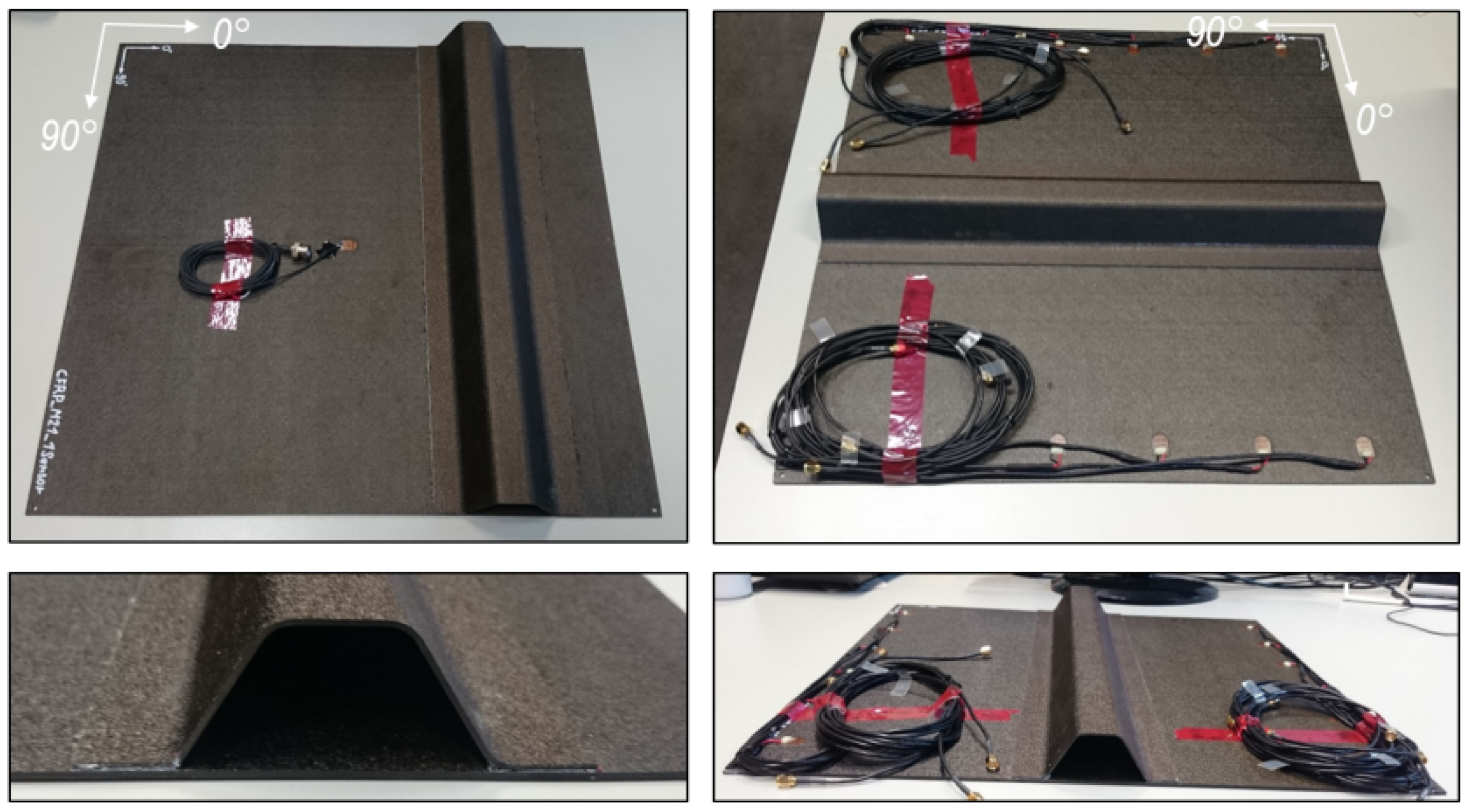
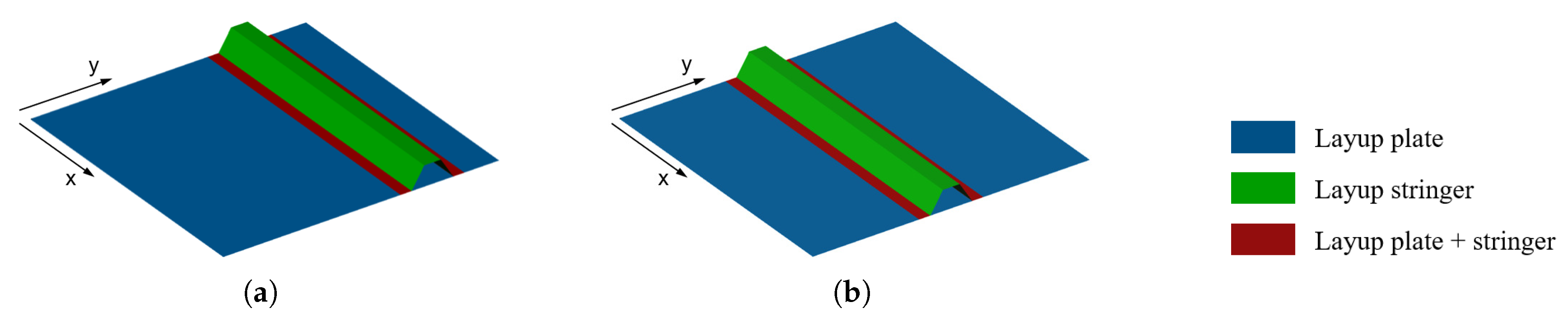
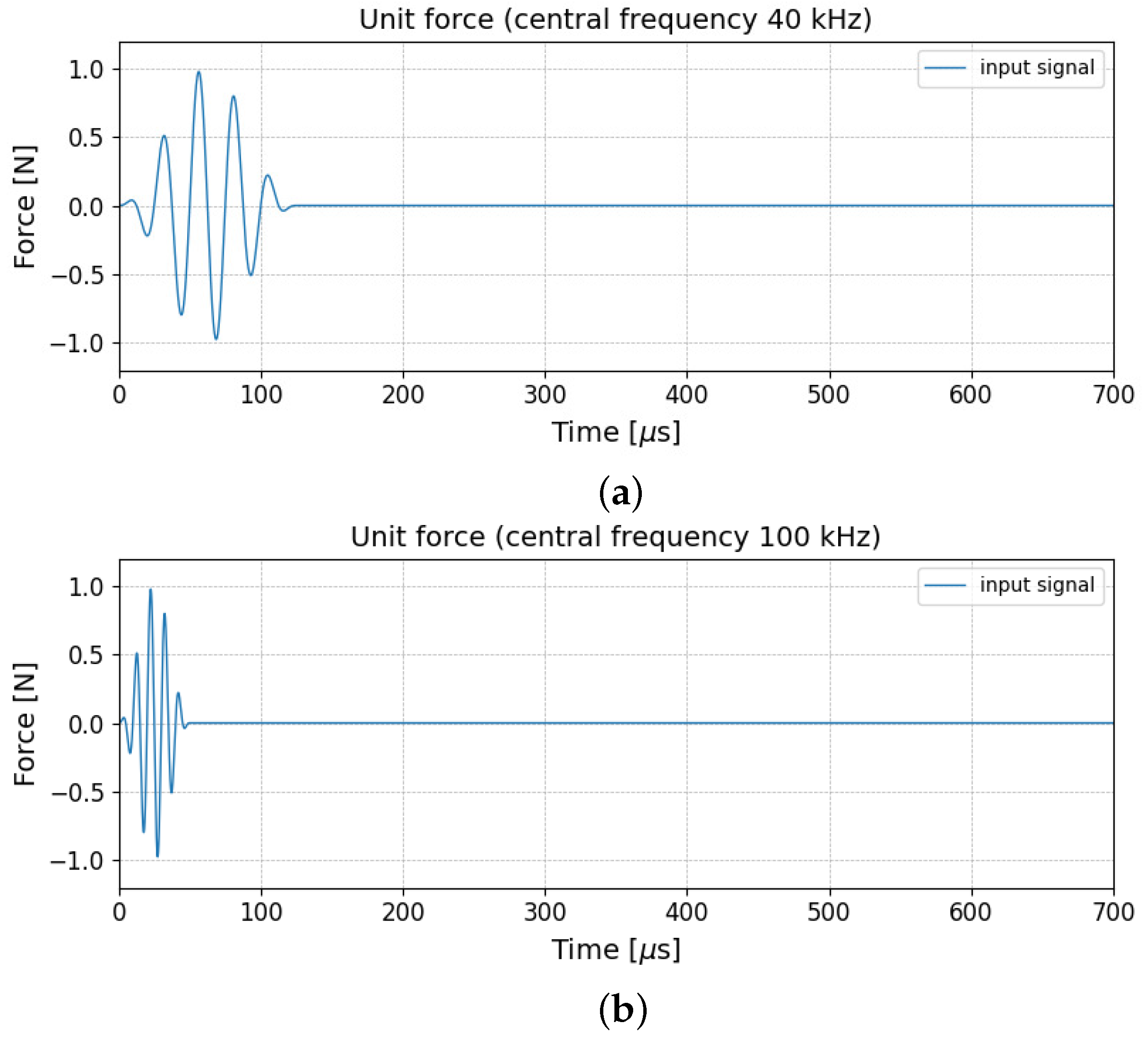
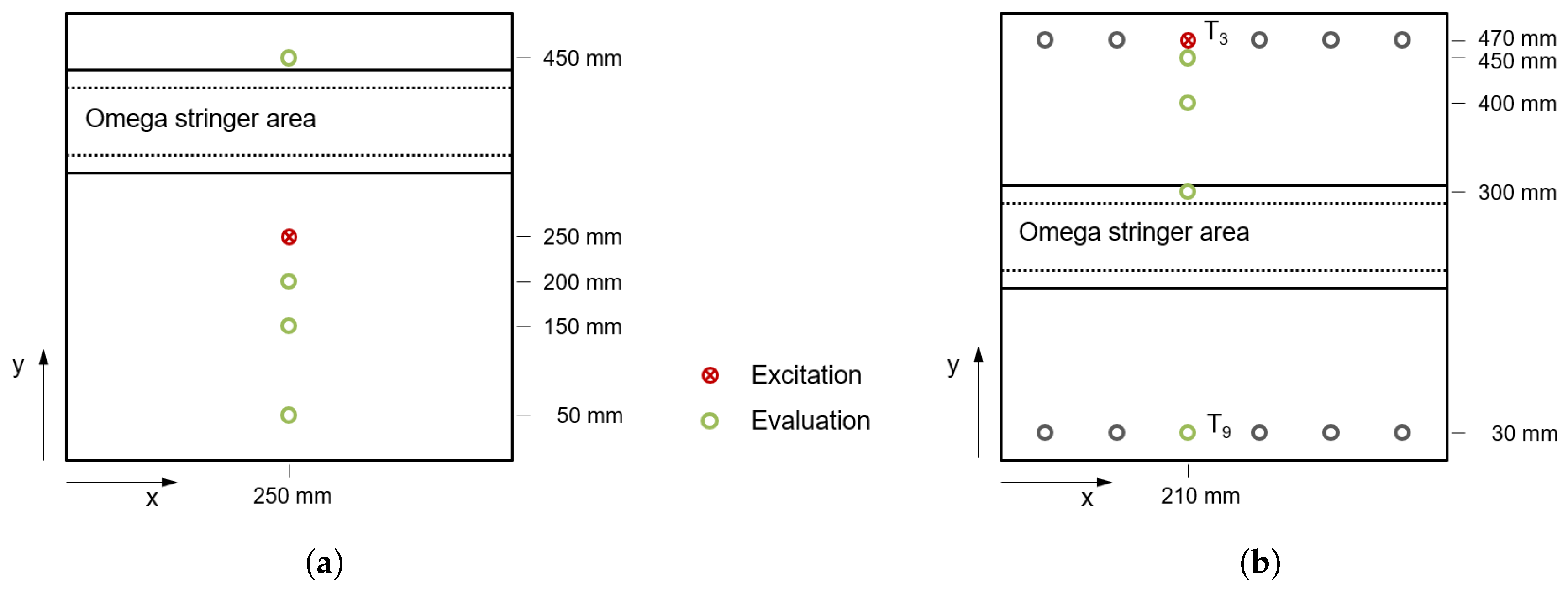
2. Experimental Setup-Open Guided Waves

For a realistic comparison of two different numerical methods, their results must first be validated with experimental data. Validating simulations is a challenging procedure for UGW, as obtaining complete and precise knowledge of the wavefield is difficult due to UGW being significantly dependent on environmental conditions. Therefore, simulations and experiments must be executed with as much sensitivity as possible. In this work, the validation was conducted on data provided by the Open Guided Waves (OGW) group [25,26], as the measurements and testing procedures of the mechanical properties of the composite samples were performed with great sensitivity, thereby increasing the possibility of conformity between experiments and simulations. The recently published new OGW dataset provides the experimental data of UGW propagation in carbon fiber composite plates with an additional omega stringer at constant temperature conditions. Two different cases have been measured in the dataset with similar plates. The composite panels with stringers are 16-layer CFRP panels of dimensions $500\times 500\times 2$ mm³. As seen in Figure 1, in the first experiment, the propagated wavefield was measured by a 3D laser Doppler vibrometer for the plate called ‘wavefield plate’, which was instrumented by a piezoelectric actuator in its center. In the second experiment, the plate called ‘SHM plate’ with the same dimensions but with a different location of the stringer was experimented. Twelve piezoelectric transducers were placed to the plate, and all the time signals were recorded for each path. In

Table 1. Plate material: transversely isotropic elastic properties for Hexply^® M21/34%/UD134/T700/300 (uni-directional) [25].

Elastic Coefficient/Density	Value	Unit
$E_{11}$	125,462	Mpa
$E_{22}$	8701	MPa
${\nu }_{12}$	0.372	-
$G_{12}$	4200	MPa
$G_{23}$	3000	MPa
$\rho$	1.571 × 10${}^{-9}$	kg/mm3

and

Table 2. Stringer material: transversely isotropic elastic properties for Hexply^® M21/34%/UD194/IMA-12K (uni-directional) [25].

Elastic Coefficient/Density	Value	Unit
$E_{11}$	171,500	MPa
$E_{22}$	8659	MPa
${\nu }_{12}$	0.324	-
$G_{12}$	5882	MPa
$G_{23}$	3331	MPa
$\rho$	1.580 × 10${}^{-9}$	kg/mm3

, the elastic property values of the used materials for the plate and stringer are listed. The lay-up configuration for the plate is ${\left[45/0/-45/90/-45/0/45/90\right]}_S$ and for the stringer is ${\left[-45/0/90/45/90/-45\right]}_S$ [25]. Consequently, the cross-sections of the plate and the stringer exhibited quasi-isotropic behavior. Figure 2 displays the lay-up distribution over the two samples. The main parameters of this experiment are mentioned; for more detailss the reader is recommended to refer to [25,26,27].

3. Numerical Modeling of Ultrasonic Guided Wave Propagation

In this section, the theoretical background of the two numerical methods that were employed to simulate ultrasonic guided wave propagation is presented very briefly. The aim is to show the main ideas behind the proposed techniques and to point out some differences.

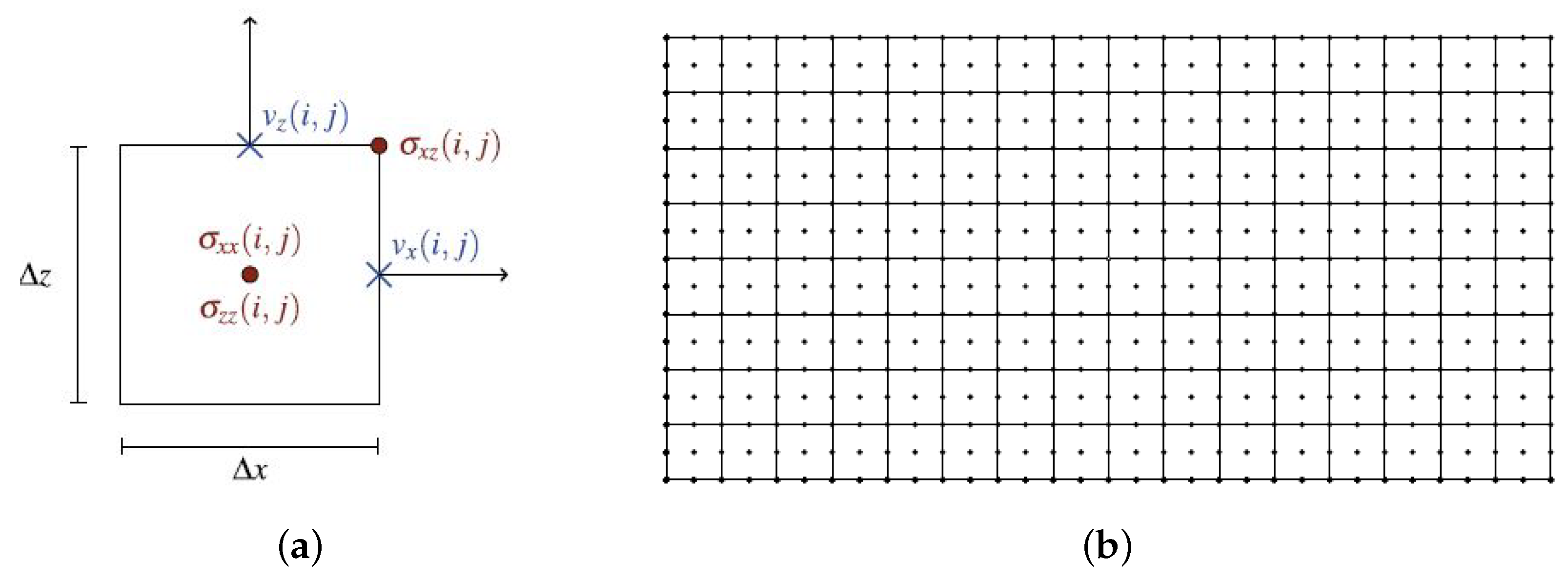
3.1. Analysis by Elasto-Dynamic Finite Integration Technique

EFIT is a stable and efficient numerical scheme to investigate all kinds of elastic wave propagation. EFIT advances with a velocity–stress formulation on a staggered spatial and temporal grid similar to the velocity–stress finite difference method (VS-FDM) introduced by Virieux [28] but on the integral form of equations instead of the differential form. To increase the comprehensibility of the scheme, one component from the stress and velocity will be derived in the following.

The propagation of elastic waves in an in-homogeneous medium is governed by Cauchy’s equation of motion

$$\rho \frac{{\partial }^2\mathbf{u}}{\partial t^2}=\nabla ·\mathit{\sigma }+\mathbf{f}$$

(1)

where $\rho =\rho (x,y,z)$ is the mass density, $\mathbf{u}=\left(u_x,u_y,u_z\right)$ is the displacement vector, $\mathit{\sigma }={\left\{{\sigma }_{i,j}\right\}}_{i,j=x,y,z}$ is the stress tensor, and $\mathbf{f}=\left(f_x,f_x,f_z\right)$ denotes the body forces. In the case of linear deformations, Hooke’s law assesses

$$\mathit{\sigma }=\mathbf{C}:\mathit{\epsilon }$$

(2)

where ε denotes the strain

$$\mathit{\epsilon }=\frac{1}{2}\left(\nabla \mathbf{u}+{(\nabla \mathbf{u})}^{\mathrm{T}}\right)$$

(3)

and $\mathbf{C}$ is the fourth order elasticity tensor containing up to 21 independent elastic constants for the anisotropic materials. Equation (1) is transformed into a hyperbolic system of the order one by introducing the particle velocity $\mathbf{v}=\partial \mathbf{u}/\partial \mathrm{t}$. We obtain [28]

$$\rho \frac{\partial \mathbf{v}}{\partial t}=\nabla ·\mathit{\sigma }+\mathbf{f}$$

(4)

and

$$\frac{\partial }{\partial t}\mathit{\sigma }=\mathbf{C}:\frac{\partial }{\partial t}\mathit{\epsilon }.$$

(5)

The basic idea of finite volume methods is to perform an integration of the differential Equations (4) and (5) over a defined volume, which is known as the so-called control volume. For readability, formulation is shown only for the two-dimensional case in the x–z-plane as mentioned. The integral form of Equation (4) over such a control volume V reads

$${\int }_V\left(\rho \frac{\partial v_x}{\partial t}\right)dV={\int }_V\left(\frac{\partial {\sigma }_{xx}}{\partial x}+\frac{\partial {\sigma }_{xz}}{\partial z}+f_x\right)dV.$$

(6)

Using the divergence theorem, we transfer Equation (6) into

$${\int }_V\left(\frac{\partial {\sigma }_{xx}}{\partial x}+\frac{\partial {\sigma }_{xz}}{\partial z}+f_x\right)dV={\int }_S\left(\left({\sigma }_{xx},{\sigma }_{xz}\right)·\mathbf{n}\right)dS+{\int }_V{f}_{x}dV$$

(7)

where $\mathbf{n}$ is the outer normal vector of the boundary edge (2D and 3D) or surface (3D) S. Technically, V can be an arbitrarily shaped volume with a sufficiently smooth boundary S. However, the most-used grid cells are Cartesian ones. Figure 3 shows the implemented staggered case that is often used for elasto-dynamic problems.

By assuming the staggered spatial grid and applying the midpoint rule to the cell $i,j$, we obtain a numerical quadrature scheme from Equations (6) and (7), which reads to complete the EFIT procedure with leap frog implementation. Every component of the wave propagation is discretized by employing almost the same procedure. Please note that no interpolation functions are necessary, and implementation of any kind of material is possible with the EFIT scheme, as every grid cell of the EFIT mesh can contain different material properties. For further information, the reader is recommended to refer [22].

3.1.1. Material Modeling

The carbon-reinforced composite plate is a multi-layered material composed of lamina layers. Modeling such structures is possible with the elasto-dynamic material parameters of a single lamina, which are known to most numerical solvers, including the EFIT. Two mainstream approaches are commonly used to represent the true material properties in composite modeling. The layer-wise method (LW) involves modeling each lamina as one or more material cells in the thickness direction, depending on their orientation. However, since a single ply in composites is usually very thin, the size of a cell would be very small in the thickness direction. Although LW modeling generally yields higher simulation accuracy, computational effort can be prohibitive for composite laminates with a certain number of plies in 3D simulations due to the high degree of freedom.

To significantly reduce the computational load, the equivalent single layer (ESL) approach is employed [23]. This method computes the effective stiffness by consolidating the multi-layered material properties, thus resulting in a homogenized material with equivalent stiffness to the original composite laminate. In other words, the goal is to determine a single layer with a stiffness equivalent to the whole layered material. Utilizing the ESL method alongside appropriate discretization in the thickness direction allows for a significant reduction in the required number of elements while ensuring accurate representation, thus enhancing the computational efficiency of the simulations. An essential aspect of the approach in composites is the wavelength–thickness ratio; the wave’s wavelength must be greater than the structure’s thickness to minimize additional undesired interactions. The ESL approach has been applied to model SHM systems based on UGW, particularly for plate-like structures [23,29].

In the current work, the ESL approach was implemented by following the procedure outlined in [23]. The stiffness matrix ${\mathit{C}}_{\mathrm{avg}}$ for the homogenized material is obtained by calculating a weighted sum of the stiffness matrices of each individual lamina, thereby taking into account their thickness and lay-up configuration. The homogenized stiffness matrix is evaluated via the following relation:

$${\mathit{C}}_{\mathrm{avg}}=\sum _{k=1}^n\left(h_k/H\right){\mathit{C}}_{\mathit{k}}$$

(8)

where ${\mathit{C}}_{\mathrm{k}}$ and $h_k$ represent the stiffness matrix and lamina thickness of the particular layer layer, respectively. This is obtained by applying transformation to the stiffness matrix.

$${\mathit{C}}_{\mathit{k}}={\mathit{R}}^T\mathit{C}\mathit{R}$$

(9)

and

$$\mathrm{R}=\left(\begin{array}{cccccc}{m}^2& n^2& 0& 0& 0& 2mn\\ n^2& m^2& 0& 0& 0& -2mn\\ 0& 0& 1& 0& 0& 0\\ 0& 0& 0& m& -n& 0\\ 0& 0& 0& n& m& 0\\ -mn& mn& 0& 0& 0& m^2-n^2\end{array}\right),m=cos\theta ,n=sin\theta$$

(10)

where $\mathit{C}$ is single uni-directional lamina with a stiffness matrix calculated by OGW authors [26] using effective material parameters of the composite lamina, and $\mathit{R}$ is the transformation matrix with respect to the rotation over the z-axis for angle $\theta$.

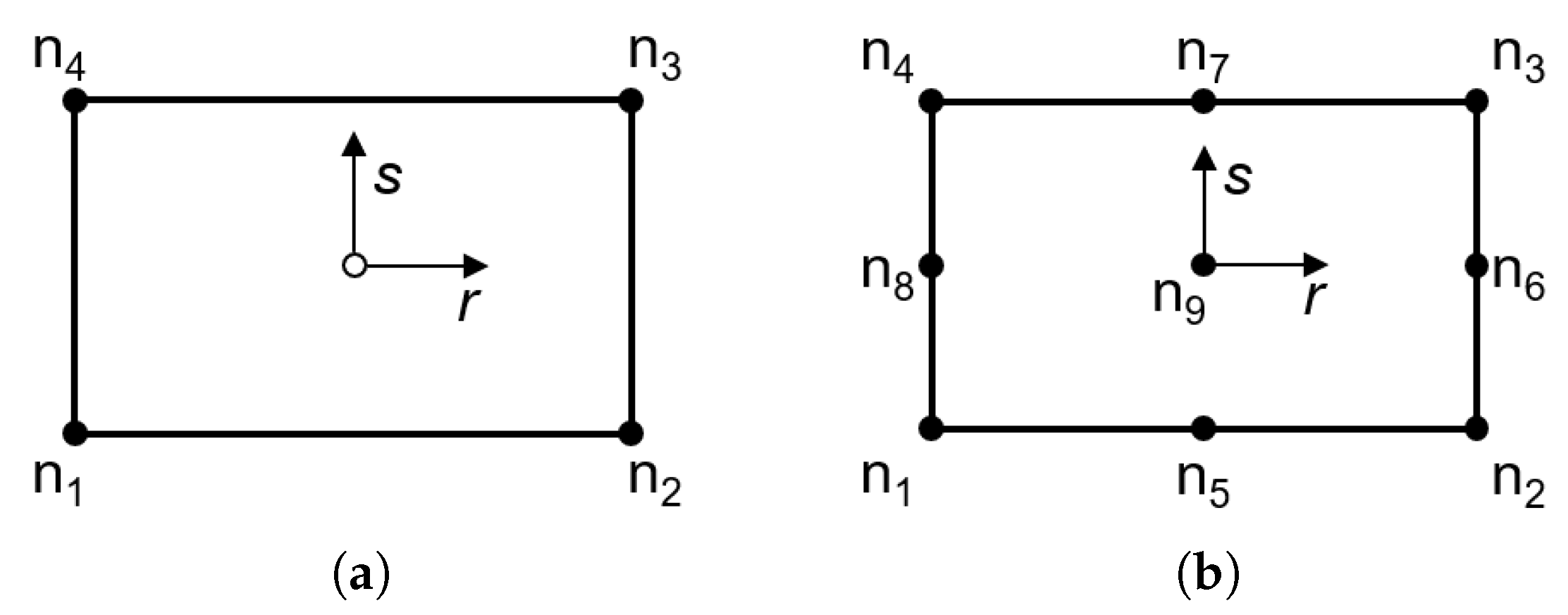
3.2. Analysis by Using Finite Shell Elements

The finite element method (FEM) is a well-suited method to perform simulations in different fields of engineering [7,8,9,12]. It is applied to solve the described partial differential equations numerically. Therefore, the whole investigated domain is discretized into single elements that are connected by their nodal values.

In order to derive the finite element discretized equations of motion, we may use Hamilton’s principle [30]

$$\delta \underset{t_0}{\overset{t_1}{\int }}\left(\mathcal{L}+\mathcal{W}\right)\mathrm{d}t=0$$

(11)

as a variation formulation of the elasto-dynamic problem. In Equation (11), $\mathcal{L}$ represents the Lagrangian function, and $\mathcal{W}$ represents the work done by external forces. By introducing the displacements $\mathbf{u}$, the mechanical stresses $\overline{\mathit{\sigma }}$, and the mechanical strains $\overline{\mathit{\epsilon }}$ of an elastic body, as well as the mass density $\rho$, the Lagrangian is received as

$$\mathcal{L}=\frac{1}{2}\underset{V}{\int }\left(\rho {\dot{\mathbf{u}}}^T\dot{\mathbf{u}}-{\overline{\mathit{\epsilon }}}^T\overline{\mathit{\sigma }}\right)\mathrm{d}V$$

(12)

and the contributions of external forces are received as

$$\mathcal{W}=\underset{V}{\int }{\mathbf{u}}^T{\mathbf{f}}_V\mathrm{d}V+\underset{S}{\int }{\mathbf{u}}^T{\mathbf{f}}_S\mathrm{d}S+\sum _{i=1}^n{\mathbf{u}}_i^T{\mathbf{f}}_i.$$

(13)

The expressions $\overline{\mathit{\sigma }}$ and $\overline{\mathit{\epsilon }}$ refer to the so-called Voigt notation collecting the components of the symmetric stress and strain tensor

$$\overline{\mathit{\sigma }}={\left[\begin{array}{cccccc}{\sigma }_{xx}& {\sigma }_{yy}& {\sigma }_{zz}& {\sigma }_{xy}& {\sigma }_{xz}& {\sigma }_{yz}\end{array}\right]}^T$$

(14)

$$\overline{\mathit{\epsilon }}={\left[\begin{array}{cccccc}{\epsilon }_{xx}& {\epsilon }_{yy}& {\epsilon }_{zz}& {\epsilon }_{xy}& {\epsilon }_{xz}& {\epsilon }_{yz}\end{array}\right]}^T.$$

(15)

We now consider Hooke’s law from Equation (2) as

$$\overline{\mathit{\sigma }}=\overline{\mathbf{C}}\overline{\mathit{\epsilon }}$$

(16)

where the elasticity matrix $\overline{\mathbf{C}}$ combines stresses $\overline{\mathit{\sigma }}$ and strains $\overline{\mathit{\epsilon }}$; a variational formulation is obtained from Equation (11) as [6]

$$\begin{array}{ccc}\hfill 0=& -& \underset{V}{\int }\left(\rho \delta {\mathbf{u}}^T\ddot{\mathbf{u}}+\delta {\overline{\mathit{\epsilon }}}^T\overline{\mathbf{C}}\overline{\mathit{\epsilon }}\right)\mathrm{d}V\hfill \\ & +& \underset{V}{\int }\delta {\mathbf{u}}^T{\mathbf{f}}_V\mathrm{d}V+\underset{S}{\int }\delta {\mathbf{u}}^T{\mathbf{f}}_S\mathrm{d}S+\sum _{i=1}^n\delta {\mathbf{u}}_i^T{\mathbf{f}}_i.\hfill \end{array}$$

(17)

By following a standard finite element procedure, the unknown displacements $\mathbf{u}$ are approximated by using shape functions $\mathbf{N}$ (space-dependent) and the nodal degrees of freedom $\mathbf{U}$ (time-dependent) of the element.

$$\mathbf{u}\left(\mathbf{x},t\right)=\mathbf{N}\left(\mathbf{x}\right)\mathbf{U}\left(t\right).$$

(18)

The differential operator $\mathbf{D}$ yields the strain–displacement relation

$$\overline{\mathit{\epsilon }}=\mathbf{Du}=\mathbf{DNU}.$$

(19)

From the fundamental lemma of the calculus of variation, we finally obtain the discretized equations of motion of the assembled system

$$\mathbf{M}\ddot{\mathbf{U}}\left(t\right)+\mathbf{KU}\left(t\right)=\mathbf{F}\left(t\right)$$

(20)

where $\mathbf{M}$ is the global mass matrix, $\mathbf{K}$ is the global stiffness matrix, and $\mathbf{F}$ is the global load vector.

Recently, the German Aerospace Center (DLR) introduced the B2000++Pro software suite [31] for research and development. This general purpose finite element analysis tool contains very efficient shell-type elements that basically follow the Reissner–Mindlin theory, which is also known as the first-order shear deformation theory (FSDT). This theory takes into account the transverse shear deformation across the shell’s thickness [32]. The displacement field $\mathbf{u}$ of the cross-section can be approximated as [33]

$$\begin{array}{ccc}\hfill u_x& =& u_x^0+z{\varphi }_x,\hfill \\ \hfill u_y& =& u_y^0+z{\varphi }_y,\hfill \\ \hfill u_z& =& u_z^0,\hfill \end{array}$$

(21)

where $u_x^0$, $u_y^0$, and $u_z^0$ are translational degrees of freedom of the element nodes, while ${\varphi }_x$ and ${\varphi }_y$ describe rotational degrees of freedom. Finite elements based on these assumptions were employed successfully to model laminated thin-walled composites [34] for guided wave analysis applications [11]. In UGW simulations, these elements have the capability to model the Lamb wave $A_0$-mode corresponding to the bending mode of the shell [15]. The Lamb wave $S_0$-mode may be detected in the very low frequency range corresponding to the membrane mode of the shell.

In spite of these limitations, the usage of conventional shell elements for analysing UGW in composite structures offers an opportunity to establish a consistent simulation set-up. As far as thin-walled lightweight structures are mainly investigated based on shell-type elements, existing models can be adapted to UGW propagation purposes easily. The transformation of existing models to 3D finite element configurations would be considerably more complex.

In contrast to a pure displacement-based element formulation, the shell elements implemented in the B2000++Pro analysis tool are of the MITC type (mixed interpolation of tensorial components), which was first introduced by Bathe et al. [35,36]. By using this kind of finite shell elements, the effect of shear locking is mostly avoided, even for distorted elements of a low nodal order [12] and despite being integrated accurately. They were also extended to analyze fiber-reinforced composite structures [37]. To perform the UGW simulation in this work, shell elements of the types Q4.S.MITC (four nodes) and Q9.S.MITC (nine nodes) [31] were used (Figure 4).

The discretized system of equations of motion (20) can be integrated numerically in the time domain by using, e.g., the implicit Newmark integration scheme [31].

4. Results

In order to compare the two proposed numerical methods, a series of simulation runs were conducted. Initially, the overall wave propagation behavior was examined between two methods, followed by an evaluation of the time-dependent displacement characteristics at specific sensor points on both the wave field plate and the SHM plate. Finally, the time-dependent velocity field of the excited wave field plate was analyzed using the EFIT and FEM; we then compared our simulation results to experimental data obtained from the OGW dataset.

For all simulation runs, the numerical models were excited by modulated out-of-plane unit forces as five-cycle Hann-windowed sine waves with different central frequencies $f_c$ [25,26]

$$\begin{array}{ccc}\hfill F\left(t\right)& =& \widehat{F}{sin}^2\left(\frac{2\pi f_{c}t}{2n}\right)sin\left(2\pi f_{c}t\right),\hfill \\ \hfill n& =& 5.\hfill \end{array}$$

(22)

In this manner, we avoided incorporating piezoelectric sensors into the numerical modeling while still allowing for the study of overall wave propagation behavior. Figure 5 displays the two different excitation signals in the time domain, which correspond to central frequencies of 40 kHz and 100 kHz and all excitation positions, as well as sensor positions for response evaluation regarding the wave field plate and the SHM plate, are shown in Figure 6.

Regarding the FEM for both samples, a model was created containing 308,000 finite shell elements possessing edge lengths of 1 mm. For the 40 kHz simulation runs, the four-node Q4.S.MITC element was employed, and, for the 100 kHz simulation runs, the nine-node Q9.S.MITC element was employed (Figure 4). In this way, the condition was ensured that the estimated wavelength of the mainly investigated Lamb wave $A_0$-mode would be covered by 15–20 nodes when using low-order techniques [16]. The finite element simulations were performed on a computer cluster using a single compute node of 128 GB RAM. For each transient simulation run, a time step size of $\Delta t=1.4\times {10}^{-7}$ s was chosen. By regarding 3000 time steps in total, wave propagation periods of 420 μs were simulated. In the case of the four-node Q4.S.MITC shell elements usage, a computation time of 2 h 30 min was needed. When employing the nine-node Q9.S.MITC shell elements, this computation time was raised to 20 h 30 min due to the increased number of degrees of freedom.

When the EFIT method was considered, the stringer and the plate were modeled according to the ESL method mentioned in Section 3.1.1. The entire area to be discretized is shown in Figure 1 with a size of $500\times 500\times 2$ mm³. The grid step size was chosen as $dx=dy=1$ mm for the plane directions and $dz=0.5$ mm for the thickness direction, which fell within the 20–40 nodes per wavelength range, thus resulting in nearly 2 million cells to be computed. EFIT simulations use a smaller time step by definition [20], so a time step of $\Delta t=3.4\times {10}^{-8}$ s was chosen, which yielded 11,500 time steps for the 420 $\mu$ simulation period. The total computation time for each transient solution was slightly less than 2 h and required just 8 GB RAM in a medium level workstation that had a 256 GB RAM capacity.

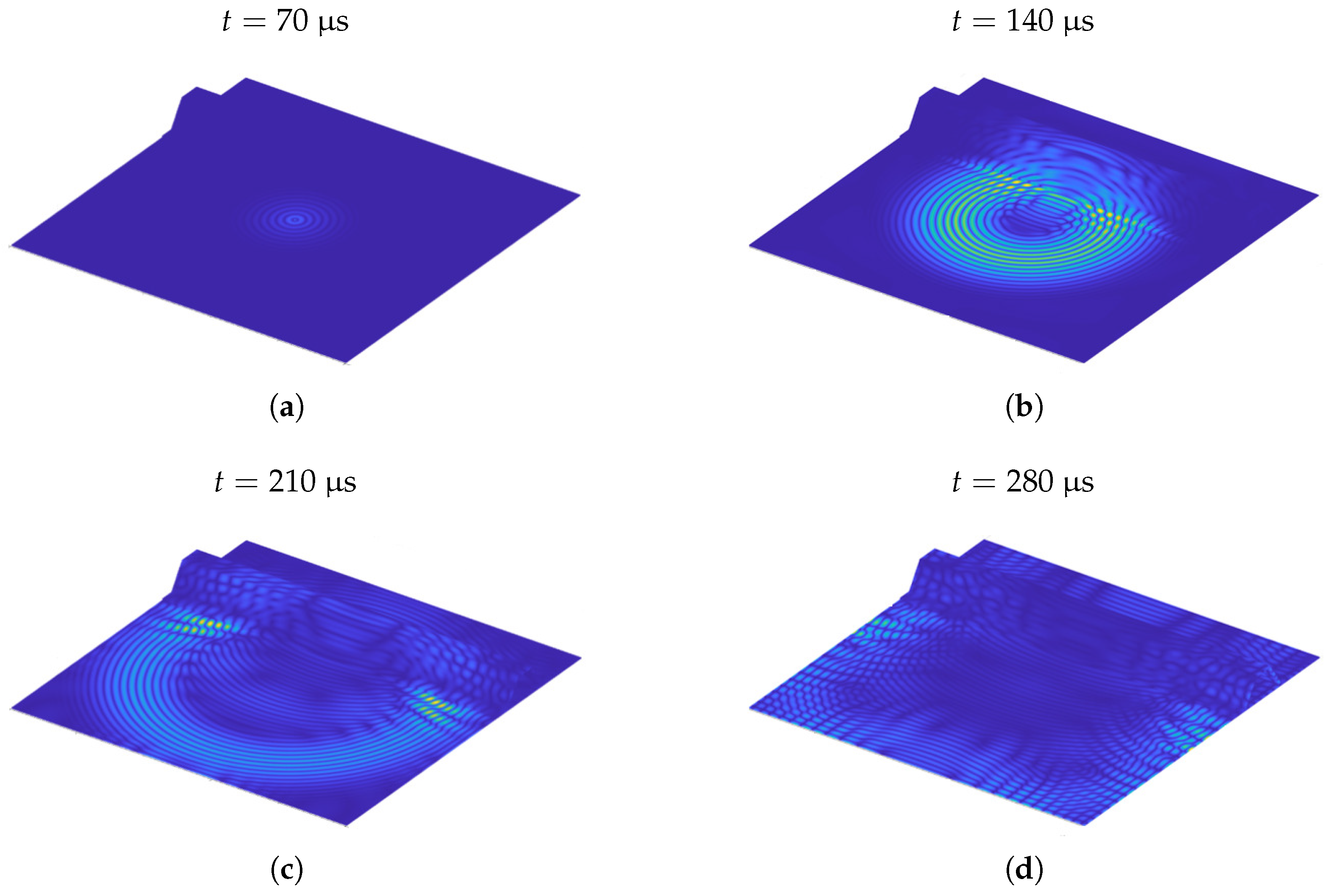
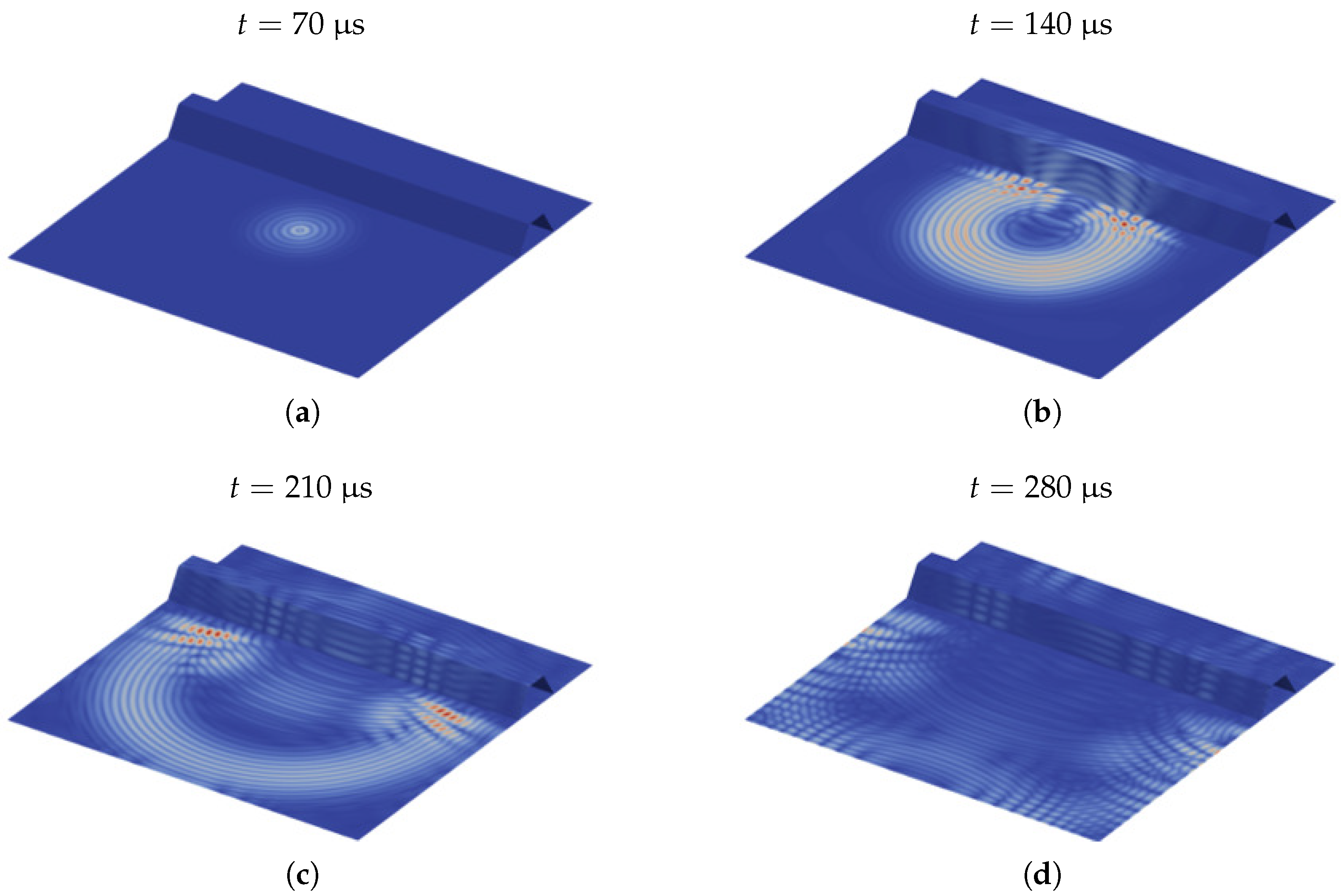
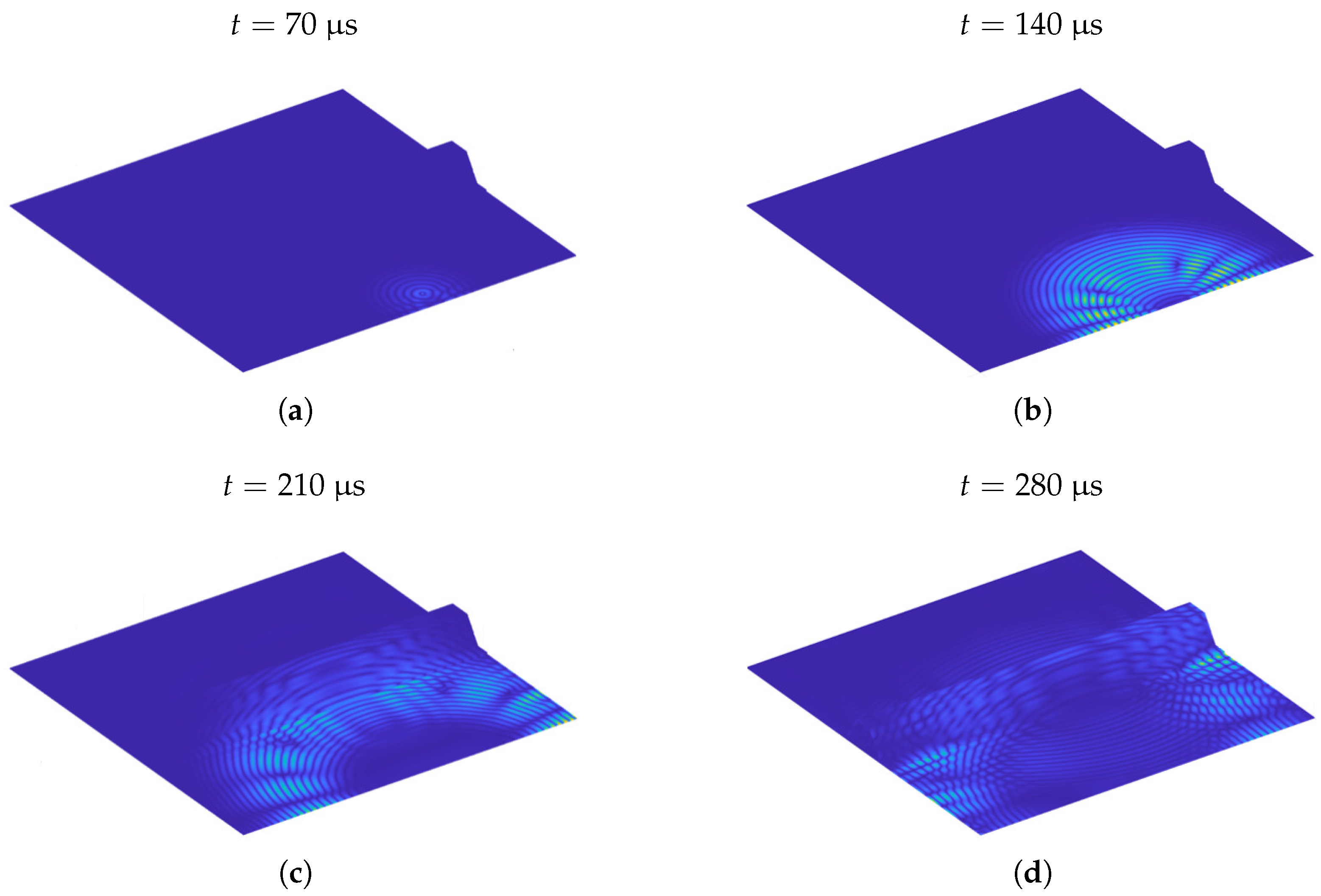
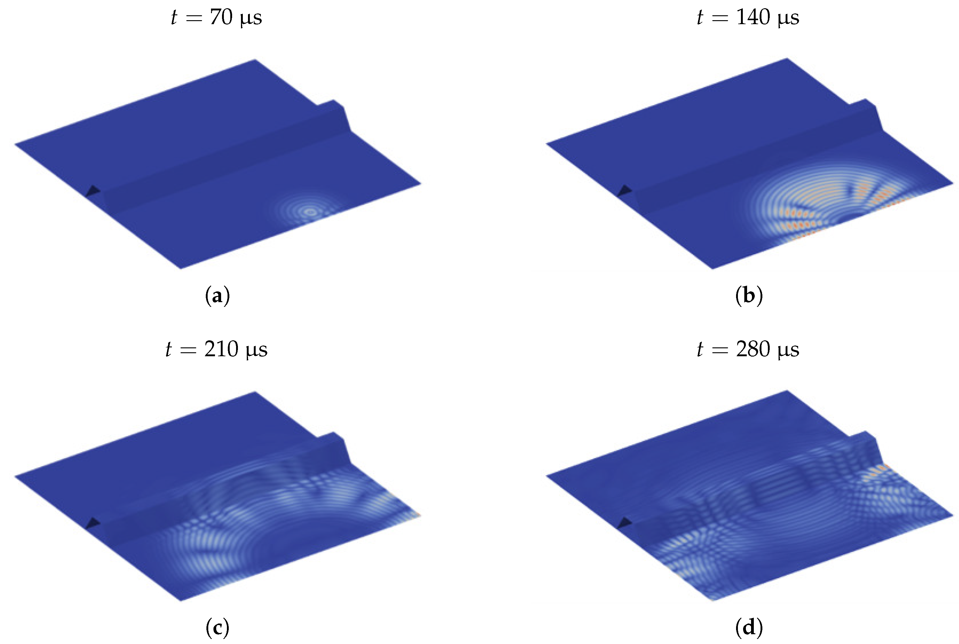
4.1. Simulated Wave Propagation Fields

In order to obtain a rough overview and general understanding how the EFIT and FEM performed in UGW applications, snapshots of wave propagation patterns for different analysis cases were compared. The captured figures depict the normalized total displacement amplitudes, thereby enabling a comparison between wave fields originating from distinct excitation scenarios such as piezoelectric transducers and single forces.

Initially, the wave field plate was considered. It was excited at the center point of the plate ($x=250$ mm/$y=250$ mm) [25] by a carrier frequency of 40 kHz. The figures present a very good match regarding the wave propagation patterns in the EFIT (Figure 7) and FEM (Figure 8) simulations. This also includes the effects of wave reflections coming from the stringer, as well as from the edges of the plate, in a general manner. The SHM plate behaved in a similar manner in simulations using the EFIT (Figure 9) and FEM (Figure 10). The SHM plate was excited near to an edge at ($x=210$ mm/$y=470$ mm). This position corresponds to the transducer T3 in the OGW data [25].

4.2. Simulated Time-of-Flight Characteristics

In this section, detailed investigation was conducted for the time-of-flight characteristics derived from the simulation results of both the EFIT and FEM methods. Our aim was to gain a deeper understanding of the performance of each numerical method in simulating ultrasonic guided wave propagation in composite materials. To ensure a thorough comparison, we focused on the displacement behavior at specific points on the SHM plate over time, thereby examining the normalized out-of-plane displacement component to enhance the comparability of the results. With respect to the finite shell elements, this part of the displacement was associated with the Lamb wave $A_0$-mode deformation, as shell elements of the used configuration were not able to reproduce the $S_0$-mode transverse displacement portion.

Wavefields were analyzed for the time-displacement histories at four specifically chosen points along the T3–T9 path of the SHM plate, as described in [25]. These points were selected based on their positions relative to the excitation location and the stringer, thereby providing a diverse set of scenarios for comparison. Figure 11a–c are related to the sensor y-locations of 450 mm, 400 mm, and 300 mm, respectively. Additionally, this choice made it possible to assess the influence of various factors, such as wave reflections, scattering, and mode conversions, on the performance of each numerical method.

In our analysis, fairly close agreement between the EFIT and FEM results for the first passing wave package was observed, with the EFIT calculated wave exhibiting a slightly slower propagation. This observation suggests that the finite element model behaves more stiffly than the EFIT model. However, when examining the displacement signals affected by the superposition of reflected and scattered waves, we observed more significant differences between the EFIT and FEM results. In particular, as seen in Figure 11d, the data recorded at the sensor position of $y=30$ mm demonstrated a higher level of deviation, as the incoming wave needed to traverse the stringer and the entire plate before being captured. This finding highlights the importance of considering the complex wave interactions within the composite structure when evaluating the performance of numerical methods for simulating ultrasonic guided waves.

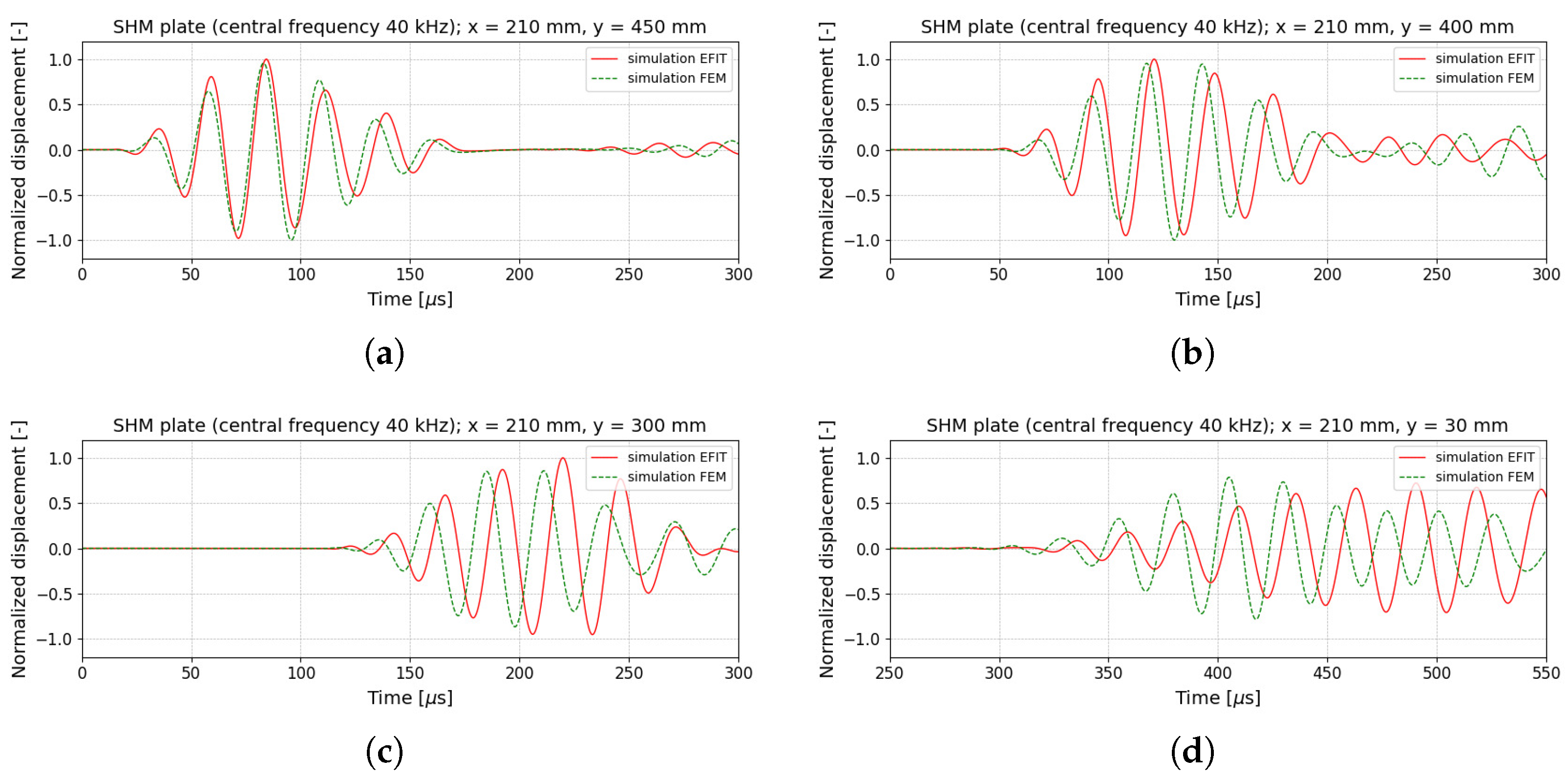
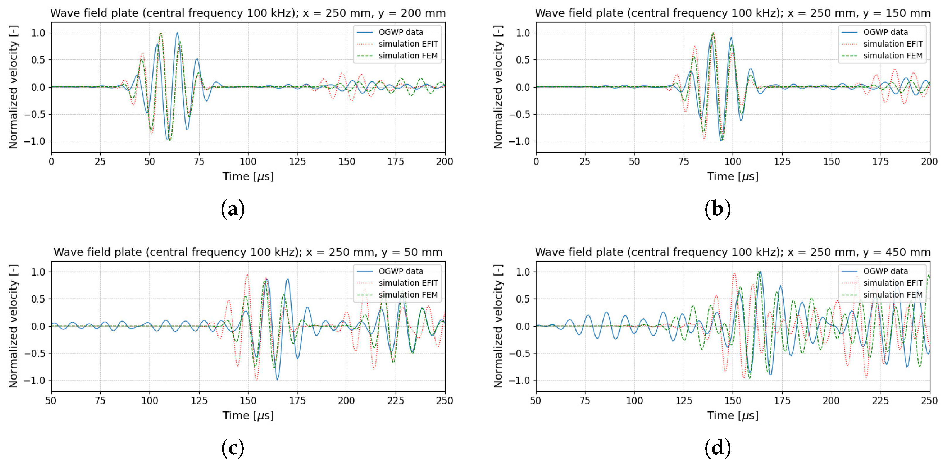
4.3. Comparison with Experimental Data

Finally, simulated wave propagation patterns and time-of-flight characteristics were compared to measured data from the OGW. This comparison was performed considering a carrier frequency of 100 kHz, thereby allowing the reported simulations to represent two different frequency levels for estimation.

The OGW datasets described in [27] contain velocity distributions for the entire wave field plate with a stringer. For the evaluated 100 kHz case, the out-of-plane velocity amplitudes obtained from measurement, as well as the EFIT and FEM outputs, are presented in Figure 12. The snapshots were taken at 140 μs after the beginning of excitation and display the surface of the wave field plate opposite the stringer. It can be observed that the results from the simulations exhibited ideal symmetric behavior, as seen in Figure 12b,c. The slight asymmetry in Figure 12a may indicate imperfections in the material properties and lay-up of the manufactured sample. It also may have resulted from asymmetries in excitation, such as uncertainties of the transducer coupling to the plate or uncertainties of the transducer itself.

Figure 13 contains the velocity time-of-flight behavior recorded at four points that were perpendicular to the stringer at $x=250$ mm (median line of the plate). As remarked for the 40 kHz case, the first propagating wave package was reproduced quite well by the EFIT and FEM, as shown in Figure 13a–c. Now, the reduced time shift of the EFIT compared to Figure 11 points to the conclusion that, in this case, both numerical methods yielded a similar phase velocity. It has to be considered that, for this FEM simulation that was run, nine-node elements of the quadratic order were used. Figure 13d represents the velocity signal after crossing the stringer. As described for the SHM plate data in Figure 11 at this position, more differences occurred due to the long wave propagation distance and scattering effects. Furthermore, it should be mentioned that the measured velocity may have also contained transverse components resulting from the Lamb $S_0$-mode that were not reproduced by the finite shell elements of the introduced type.

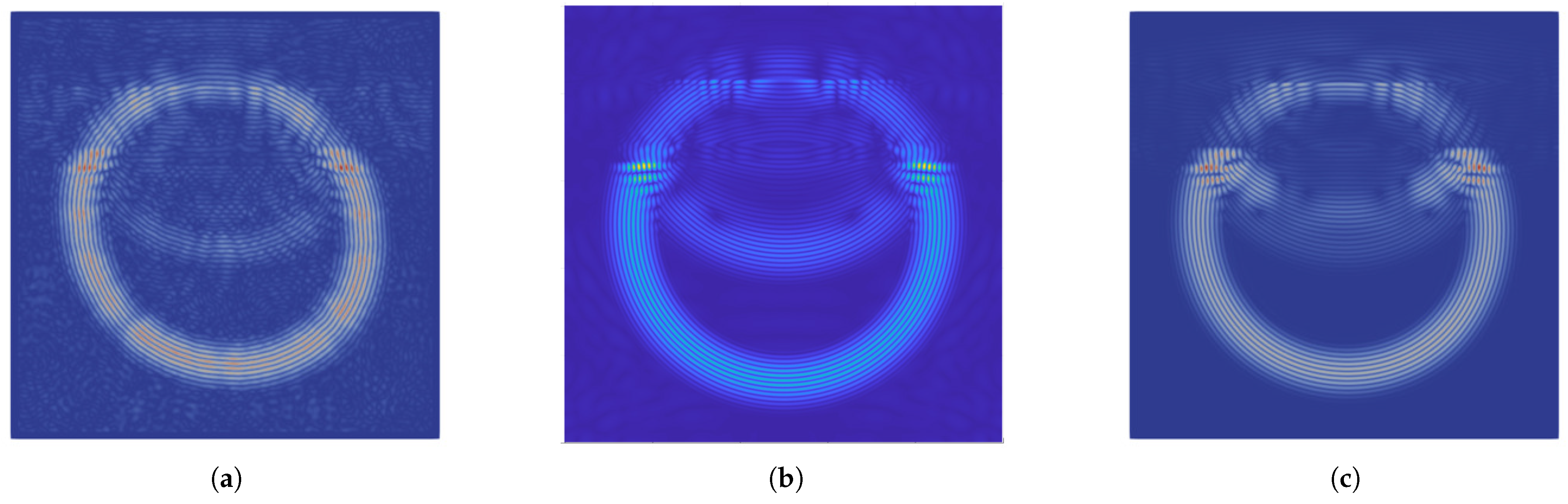
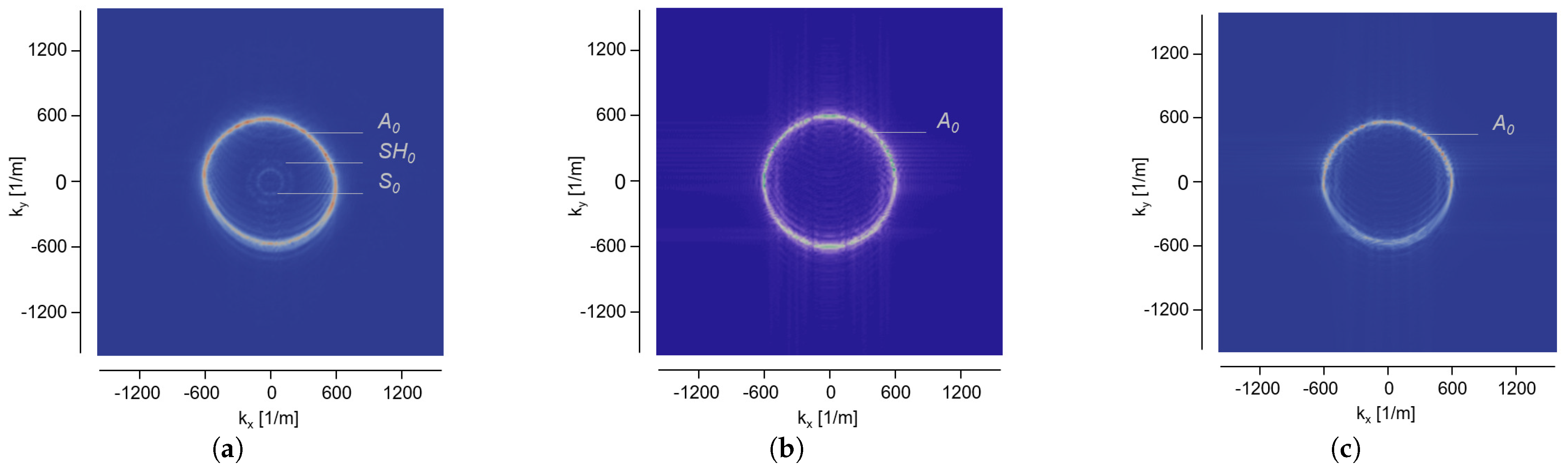
4.4. Transformation to Wavenumber–Frequency Domain

In order to get more information about the guided wave propagation characteristics, a three-dimensional fast Fourier transformation (3D-FFT) can be applied to the transient wavefield data [38]. Thus, the data sets were transformed from the space–time domain (x direction, y direction, t) to the wavenumber–frequency domain (wavenumber $k_x$, wavenumber $k_y$, f) [39]. The wavenumber plots show the dispersion behavior of the propagating waves for different mode types. Additionaly, the wavenumber plots provide valuable information about the directionality of wave propagation in the structure. In the $k_x{k}_y$ plane, the direction of wave propagation can be inferred from the orientation and distribution of energy [16].

As was already mentioned, concerning the composite structure the wave propagation field in Figure 12, the wavenumber plot of the experimental data Figure 14a shows imperfections in the material property distribution due to a remaining variety of unknowns. By contrast, the wavenumber plot based on the simulation data in Figure 14b,c exhibit symmetry in the x and y direction. However, the dominant wave mode and its spatial frequencies exhibited a fair match between the simulations and experiments. All three plots estimated a Lamb $A_0$-mode wavenumber of about 600 1/m for the 100 kHz case. In Figure 14a, referring to the experimental data set, the wavenumber profiles of the shear horizontal $S{H}_0$-mode and the Lamb $S_0$-mode can also be observed very slightly. Naturally, the incidence of these modes was not possible in Figure 14b,c due to the reasons mentioned in the previous chapter.

5. Conclusions

In this work, the application of two distinct numerical methods for ultrasonic guided wave analysis has been demonstrated. The EFIT method possesses the advantage of being fundamentally a 3D technique, which can be adapted to investigate various wave propagation phenomena. Low-order finite shell elements are commonly utilized in a large variety of software tools and enable the creation of complex models. However, they have the disadvantage of being originally developed for strength analysis and considerations concerning the global dynamic behavior of the structure. Hence, low-order finite shell elements are not capable of reproducing all deformation characteristics related to UGW propagation. Nevertheless, it was shown that it is possible to obtain similar results from both numerical methods. These results were also verified by experimental data from the OGW. In particular, the Lamb wave $A_0$-mode, which has a great importance for damage detection in thin-walled structures, could be captured quite well.

In future steps, more simulation runs should be conducted and compared to consider aspects such as convergence behavior related to different sizes of elements and time steps to explore the limitations and capabilities of both methods for such complex structures. Moreover, it is crucial to investigate how the propagating wave field is influenced by reflection effects originating from edges, geometrical discontinuities, material imperfections, and damage. In particular, the effects arising from the superposition of reflected and scattered waves must be studied with great precision. A detailed comparison of both numerical methods also should include the development of an appropriate quantification strategy. Such a strategy might be based on signal energy criteria, as proposed in [25], to evaluate the time-depending behavior at different observation points. Another approach could use the information coming from the transformations to the wavenumber–frequency domain, as well as comparing statistical measures.

In addition, the finite shell element formulation currently implemented in B2000++Pro software suite should be enhanced to reproduce more aspects of Lamb wave deformation behavior. This could be accomplished by introducing the out-of-plane normal strain as an additional nodal degree of freedom [40]. This concept has already been applied to UGW analysis [41]. Improved modeling capabilities with respect to the Lamb wave $S_0$-mode may also enable the numerical investigation of mode conversion phenomena [42]. These effects are important for damage detection purposes. Furthermore, the shell element improvement can be the starting point for a more detailed dispersion analysis. Regarding the EFIT implementation, the incorporation of more advanced and realistic averaging techniques using equivalent single layer theory for material properties could lead to improved wave propagation phenomena simulations while simultaneously reducing computational demands.

In conclusion, both numerical methods presented here appear to be promising foundations for comprehensive probability of detection (POD) investigations with respect to damage and imperfections as anticipated in [23]. The OGW method also provides an initial approach. There are also datasets available, including an artificial reference damage. This reference damage consists of small elliptical-shaped steel plates bonded on the surface of the composite plates [25]. In this manner, the introduced analysis tools, as well as the continued research and development in this area, contribute to the development and optimization of UGW-based SHM systems.

References

1. Mitra, M.; Gopalakrishnan, S. Guided wave based structural health monitoring: A review. Smart Mat. Struct. 2016, 25, 053001. [Google Scholar] [CrossRef]
2. Su, Z.; Ye, L.; Lu, Y. Guided lamb waves for identification of damage in composite structures: A review. J. Sound Vib. 2006, 295, 753–780. [Google Scholar] [CrossRef]
3. Lee, B.C.; Staszewski, W.J. Modelling of Lamb waves for damage detection in metallic structures: Part I. Wave propagation. Smart Mat. Struct. 2003, 12, 804–814. [Google Scholar] [CrossRef]
4. Lee, B.C.; Staszewski, W.J. Modelling of Lamb waves for damage detection in metallic structures: Part II. Wave interactions with damages. Smart Mat. Struct. 2003, 12, 815–824. [Google Scholar] [CrossRef]
5. Giurgiutiu, V. Structural Health Monitoring with Piezoelectric Wafer Active Sensors; Academic Press (Elsevier): Amsterdam, The Netherlands, 2008. [Google Scholar]
6. Willberg, C.; Duczek, S.; Vivar-Perez, J.M.; Ahmad, Z.A.B. Simulation methods for guided wave-based structural health monitoring: A review. Appl. Mech. Rev. 2015, 67, 010803. [Google Scholar] [CrossRef]
7. Zienkiewicz, O.C.; Taylor, R. The Finite Element Method. The Basis, Vol. 1; Butterworth-Heinemann: Oxford, UK, 2000. [Google Scholar]
8. Zienkiewicz, O.C.; Taylor, R. The Finite Element Method. Solid Mechanics, Vol. 2; Butterworth-Heinemann: Oxford, UK, 2000. [Google Scholar]
9. Zienkiewicz, O.C.; Taylor, R. The Finite Element Method. Fluid Dynamics, Vol. 3; Butterworth-Heinemann: Oxford, UK, 2000. [Google Scholar]
10. Yang, C.; Ye, L.; Su, Z.; Bannister, M. Some aspects of numerical simulation for Lamb wave propagation in composite laminates. Comp. Struct. 2006, 75, 267–275. [Google Scholar] [CrossRef]
11. Kudela, P.; Żak, A.; Krawczuk, M.; Ostachowicz, W. Modelling of wave propagation in composite plates using the time domain spectral element method. J. Sound Vib. 2007, 302, 728–745. [Google Scholar] [CrossRef]
12. Bathe, K.-J. Finite Element Procedures; Prentice Hall: Englewood Cliffs, NJ, USA, 1996. [Google Scholar]
13. Dauksher, W.; Emery, A.F. The solution of elastostatic and elastodynamic problems with Chebyshev spectral finite elements. Comput. Meth. Appl. Mech. Eng. 2000, 188, 217–238. [Google Scholar] [CrossRef]
14. Peng, H.; Meng, G.; Li, F. Modeling of wave propagation in plate structures using three-dimensional spectral element method for damage detection. J. Sound Vib. 2009, 320, 942–954. [Google Scholar] [CrossRef]
15. Ostachowicz, W.; Kudela, P.; Krawczuk, M.; Żak, A. Guided Waves in Structures for SHM: The Time-Domain Spectral Element Method; Wiley: Chichester, UK, 2012. [Google Scholar]
16. Mesnil, O.; Recoquillay, A.; Druet, T.; Serey, V.; Hoang, H.T.; Imperiale, A.; Demaldent, E. Experimental validation of transient spectral finite element simulation tools dedicated to guided wave-based structural health monitoring. J. Nondestruct. Eval. Diag. Prog. Eng. Sys. 2021, 4, 041003. [Google Scholar] [CrossRef]
17. Willberg, C.; Gabbert, U. Development of a three-dimensional piezoelectric isogeometric finite element for smart structure applications. Acta Mech. 2012, 223, 1837–1850. [Google Scholar] [CrossRef]
18. Ramadas, C.; Balasubramaniam, K.; Joshi, M.; Krishnamurthy, C.V. Interaction of the primary anti-symmetric Lamb mode (A0) with symmetric delaminations: Numerical and experimental studies. Smart Mater. Struct. 2009, 18, 085011. [Google Scholar] [CrossRef]
19. Mook, G.; Pohl, J.; Simonin, Y. Lamb wave generation, propagation and interactions in CFRP plates. In Lamb-Wave Based Structural Health Monitoring in Polymer Composites; Rolf Lammering, R., Gabbert, U., Sinapius, M., Schuster, T., Wierach, P., Eds.; Springer International Publishing: Cham, Switzerland, 2018; pp. 443–461. [Google Scholar]
20. Fellinger, P.; Marklein, R.; Langenberg, J.; Kloholz, S. Numerical modeling of elastic wave propagation and scattering with EFIT-elastodynamic finite integration technique. Wave Motion 1995, 21, 47–66. [Google Scholar] [CrossRef]
21. Schubert, F. Numerical time-domain modeling of linear and nonlinear ultrasonic wave propagation using finite integration techniques—Theory and applications. Ultrasonics 2004, 42, 221–229. [Google Scholar] [CrossRef] [PubMed]
22. Tschöke, K.; Gravenkamp, H. On the numerical convergence and performance of different spatial discretization techniques for transient elastodynamic wave propagation problems. Wave Motion 2018, 82, 62–85. [Google Scholar] [CrossRef]
23. Tschöke, K.; Mueller, I.; Memmolo, V.; Moix-Bonet, M.; Moll, J.; Lugovtsova, Y.; Golub, M.; Venkat, R.S.; Schubert, L. Feasibility of model-assisted probability of detection principles for structural health monitoring systems based on guided waves for fiber-reinforced composites. IEEE Trans. Ultrason. Ferroelectr. Freq. Control 2021, 68, 3156–3173. [Google Scholar] [CrossRef]
24. Leckley, C.; Wheeler, K.R.; Hafiychuk, H.; Timuçin, D.A. Simulation of guided-wave ultrasound propagation in composite laminates: Benchmark comparisons of numerical codes and experiment. Ultrasonics 2018, 84, 187–200. [Google Scholar] [CrossRef]
25. Moll, J.; Kexel, C.; Kathol, J.; Fritzen, C.-P.; Moix-Bonet, M.; Willberg, C.; Rennoch, M.; Koerdt, M.; Herrmann, A. Guided waves for damage detection in complex composite structures: The influence of omega stringer and different reference damage size. Appl. Sci. 2020, 10, 3068. [Google Scholar] [CrossRef]
26. Moll, J.; Kathol, J.; Fritzen, C.-P.; Moix-Bonet, M.; Rennoch, M.; Koerdt, M.; Herrmann, A.S.; Sause, M.G.R.; Bach, M. Open Guided Waves: Online platform for ultrasonic guided wave measurements. Struct. Health Monit. 2019, 18, 1903–1914. [Google Scholar] [CrossRef]
27. Kudela, P.; Radzienski, M.; Moix-Bonet, M.; Willberg, C.; Lugovtsova, Y.; Bulling, J.; Tschöke, K.; Moll, J. Dataset on full ultrasonic guided wavefield measurements of a CFRP plate with fully bonded and partially debonded omega stringer. Data Brief 2022, 42, 108078. [Google Scholar]
28. Virieux, J. SH-wave propagation in heterogeneous media: Velocity-stress finite-difference method. Geophysics 1984, 49, 1933–1942. [Google Scholar] [CrossRef]
29. Memmolo, V.; Monaco, E.; Boffa, N.; Maio, L.; Ricci, F. Guided wave propagation and scattering for structural health monitoring of stiffened composites. Compos. Struct. 2018, 184, 568–580. [Google Scholar] [CrossRef]
30. Tzou, H.S. Piezoelectric Shells. Distributed Sensing and Control of Continua; Kluwer Academic Publishers: Dordrecht, The Netherlands, 1993. [Google Scholar]
31. SMR Package Documentation. Available online: https://www.smr.ch/doc/ (accessed on 7 September 2022).
32. Rolfes, R.; Rohwer, K. Improved transverse shear stresses in composite finite elements based on First Order Shear Deformation Theory. Int. J. Num. Meth. Eng. 1997, 40, 51–60. [Google Scholar] [CrossRef]
33. Reddy, J.N. Theory and Analysis of Elastic Plates; Taylor & Francis: Philadelphia, PA, USA, 1999. [Google Scholar]
34. Ochoa, O.O.; Reddy, J.N. Finite Element Analysis of Composite Laminates; Kluwer Academic Publishers: Dordrecht, The Netherlands, 1992. [Google Scholar]
35. Bathe, K.-J.; Dvorkin, E.N. Short communication: A four-node plate bending element based on Mindlin/Reissner plate theory and a mixed interpolation. Int. J. Num. Meth. Eng. 1985, 21, 367–383. [Google Scholar] [CrossRef]
36. Bathe, K.-J.; Iosilevicha, A.; Chapelle, D. An evaluation of the MITC shell elements. Comp. Struct. 2000, 75, 1–30. [Google Scholar] [CrossRef]
37. Alfano, G.; Auricchio, F.; Rosati, L.; Sacco, E. MITC finite elements for laminated composite plates. Int. J. Numer. Meth. Eng. 2001, 50, 707–738. [Google Scholar] [CrossRef]
38. Malatesta, M.M.; Moll, J.; Kudela, P.; Radzieński, M.; De Marchi, L. Wavefield analysis tools for wavenumber and velocities extraction in polar coordinates. IEEE Trans. Ultrason. Ferroelect. Freq. Control 2022, 69, 399–410. [Google Scholar] [CrossRef]
39. Kudela, P.; Radzieński, M.; Fiborek, P.; Wandowski, T. Elastic constants identification of fibre-reinforced composites by using guided wave dispersion curves and genetic algorithm for improved simulations. Compos. Struct. 2021, 272, 114178. [Google Scholar] [CrossRef]
40. Whitney, J.M.; Sun, C.T. A higher order theory for extensional motion of laminated composites. J. Sound Vib. 1973, 30, 85–97. [Google Scholar] [CrossRef]
41. Żak, A. A novel formulation of a spectral plate element for wave propagation in isotropic structures. Fin. Elem. Analys. Des. 2009, 45, 650–658. [Google Scholar] [CrossRef]
42. Willberg, C.; Koch, S.; Mook, G.; Pohl, J.; Gabbert, U. Continuous mode conversion of Lamb waves in CFRP plates. Smart Mat. Struct. 2012, 21, 075022. [Google Scholar] [CrossRef]
Figure 1. Photos of the wave-field plate (left) and SHM plate (right) from [25].
Aerospace 10 00430 g001
Figure 2. Composite lay-up overview: (a) wave field plate, (b) SHM plate.
Aerospace 10 00430 g002
Figure 3. (a) Staggered grid cell i,j of the 2D EFIT scheme; (b) exemplary Grid of the EFIT.
Aerospace 10 00430 g003
Figure 4. Configuration of finite shell elements as are included in the B2000++Pro analysis package [31]: (a) Q4.S.MITC, (b) Q9.S.MITC.
Aerospace 10 00430 g004
Figure 5. Modulated out-of-plane unit forces: (a) f c = 40 kHz, (b) f c = 100 kHz.
Aerospace 10 00430 g005
Figure 6. Excitation and sensor positions overview: (a) wave field plate, (b) SHM plate.
Aerospace 10 00430 g006
Figure 7. EFIT wave field plate considering f c = 40 kHz excitation: visualization of normalized total displacement amplitude wave propagation fields.
Aerospace 10 00430 g007
Figure 8. FEM wave field plate considering f c = 40 kHz excitation: visualization of normalized total displacement amplitude wave propagation fields.
Aerospace 10 00430 g008
Figure 9. EFIT SHM plate considering f c = 40 kHz excitation: visualization of normalized total displacement amplitude wave propagation fields.
Aerospace 10 00430 g009
Figure 10. FEM SHM plate considering f c = 40 kHz excitation: visualization of normalized total displacement amplitude wave propagation fields.
Aerospace 10 00430 g010
Figure 11. SHM plate considering f c = 40 kHz excitation: comparison of time-dependent normalized out-of-plane displacements (EFIT vs. FEM) along path T3 (actuation)–T9 [25]; signal measured at (a) x = 210 mm/ y = 450 mm, (b) x = 210 mm/ y = 400 mm, (c) x = 210 mm/ y = 300 mm, and (d) x = 210 mm/ y = 30 mm.
Aerospace 10 00430 g011
Figure 12. Wave field plate considering f c = 100 kHz excitation: comparison of normalized out-of-plane velocity amplitude wave propagation fields at t = 140 μs. (a)—measurement data from OGW [27], (b)—EFIT, (c)—FEM.
Aerospace 10 00430 g012
Figure 13. Wave field plate considering f c = 100 kHz excitation: comparison of time-dependent normalized out-of-plane velocities (OGW data [27] vs. EFIT and FEM); signal measured at (a) x = 250 mm/ y = 200 mm, (b) x = 250 mm/ y = 150 mm, (c) x = 250 mm/ y = 50 mm, and (d) x = 250 mm/ y = 450 mm.
Aerospace 10 00430 g013
Figure 14. Wave field plate considering f c = 100 kHz excitation: comparison of normalized out-of-plane wavenumber profiles at 100 kHz. (a) Measurement data from OGW [27], (b) EFIT, (c) FEM.
Aerospace 10 00430 g014