A Novel System-Based Empirical Mode Decomposition with Improved Upper Bounds Applied to Environmental Datasets

Abstract

We are interested in modelling smaller datasets to generate more accurate, sub-regional or regional climate forecasts. The focus of this paper is to present the findings of a study investigating the application of empirical mode decomposition (EMD) to identify the components of the signal from which we can subsequently derive an iterated function system (IFS). One could develop a series of models, which are not based on big data, but rather allow for a cyclical model to keep the cycle iterating so that the model can be more responsive and adaptive to changes in the climate. The results presented in this paper have identified a new upper bound for the number of intrinsic mode functions (IMFs) obtained after EMD. The goal of the research is to develop a model where climate data could be iterated adaptively between models.

1. Introduction

Key Points:

• Improved upper bound for the number of EMD IMFs.
• Data-centric approach to calculating the number of IMFs.
• Evaluated on datasets and with EMD variants.

Reliable and accurate climate forecasting is becoming increasingly crucial for decision-making at various levels, from local to global. Policymakers require trustworthy projections of extreme weather events, seasonal climate behaviour, and longer-term climate shifts to support disaster preparedness and mitigation strategies. Examples of such forecasts include short-term hurricane tracking in the United States, the seasonal onset of the Indian Monsoon [1], interannual variations such as the El Niño–Southern Oscillation and its effects on European climate [2], and long-range predictions of global mean temperature changes [3]. The past decade has seen unprecedented warming trends, intensifying the frequency and severity of extreme weather phenomena [4,5]. This reinforces the need for improved methods to anticipate local, regional, and global climate risks. Global climate models (GCMs) are the primary tools used to simulate future climate conditions. While they offer large-scale insights, they are limited in their ability to resolve fine-scale features and short-term extremes [6,7]. GCMs struggle with extreme event representation [8] and can underperform compared to historical climatology [9]. These limitations stem in part from coarse spatial resolution, which causes sub-grid processes like intense rainfall to be averaged and misrepresented [10]. Additionally, key drivers such as El Niño may be poorly captured [11], and wide variability remains between models [12]. Despite continuous improvements in model physics and parameterisation, GCMs remain computationally expensive and often require tailoring to specific phenomena, reducing generalisability.

To address the shortcomings of GCMs, regional climate models (RCMs) offer an enhanced resolution that is capable of capturing mesoscale processes [13,14]. However, RCMs inherit boundary condition errors from GCMs and can also produce artefacts or biases of their own [15,16]. Moreover, post-processing steps like statistical downscaling often introduce further uncertainties [17,18]. As a result, uncertainty in localised climate predictions remains a persistent challenge [19,20].

In response to these challenges, alternative modelling approaches have increasingly explored data-driven and hybrid techniques to complement physics-based climate models. Among these, empirical mode decomposition (EMD) has emerged as a powerful adaptive method for analysing nonlinear and non-stationary environmental time series. EMD and its variants have been widely applied in atmospheric, oceanic, and climate studies to extract physically meaningful oscillatory modes without imposing predefined basis functions. However, a fundamental and persistent limitation of EMD-based approaches lies in the absence of a principled criterion for determining the number of intrinsic mode functions (IMFs) required to adequately represent a signal. In practice, the number of IMFs is treated as an emergent outcome of the algorithm and is commonly bounded heuristically by the length of the time series. This often leads to over-decomposition, reduced interpretability, and unnecessary computational overhead—issues that are particularly acute when working with sparse, regional, or short-duration climate datasets.

Our work builds on previous developments in optimisation techniques and signal decomposition for environmental time series [21], as well as system-based and fractal-inspired modelling approaches [22] that seek to capture the evolving dynamics of complex environmental systems. In line with recent probabilistic and adaptive forecasting paradigms [23], we adopt an iterative modelling philosophy that does not rely on large-scale data assimilation but instead emphasises responsiveness to changing climate signals over short- to medium-term horizons. Within this context, EMD is not used as a forecasting tool in isolation but as a structural component for constructing an adaptive system-based framework.

Accordingly, this study addresses the following research questions: (i) Can the upper bound on the number of IMFs in EMD-based decompositions be reformulated in terms of the dimensionality of environmental variables rather than the length of the time series? (ii) Does such a reformulation improve robustness, interpretability, and efficiency when modelling sparse or regional climate datasets? Addressing these questions involves several challenges, including balancing signal fidelity against over-decomposition, preserving physically meaningful interactions between variables, and ensuring that the resulting framework remains adaptable across heterogeneous environmental datasets. These challenges are critical in climate science, where data availability is often limited at regional scales, yet decision-makers require reliable and responsive forecasts.

Recent studies have demonstrated the broad applicability of EMD and hybrid EMD-based frameworks across diverse domains, reinforcing the relevance of decomposition-driven representations beyond individual application areas. For example, EMD has been combined with machine learning models for predictive tasks in respiratory motion estimation [24], sub-hourly energy load forecasting [25], medical image classification [26], and short-term wind speed prediction [27], illustrating its effectiveness in extracting meaningful intrinsic components prior to modelling. In climate-related contexts, EMD has also been applied to land surface temperature projection under changing climate conditions [28]. Collectively, these studies demonstrate that while EMD is widely adopted as a preprocessing or hybrid modelling tool, challenges remain in controlling decomposition complexity and ensuring interpretability, particularly in multivariate and data-sparse settings, motivating the contribution proposed in this study.

Building on our earlier conference contribution [29], which introduced a rapid adaptive climate modelling framework for a tidal dataset from the Bay of Fundy, this study presents an enhanced empirical mode decomposition (EMD)-based technique with refined upper bounds and broader applicability. The current paper offers a more robust theoretical foundation and applies the method to diverse environmental datasets, demonstrating improved adaptability and performance.

The remainder of the paper is structured as follows: Section 2 presents the proposed modelling framework; Section 3 details the methodological background; Section 4 introduces the variable-centric empirical contribution; Section 5 presents a case study; Section 6 discusses the simulation results; and Section 7 concludes the paper.

2. Proposed Model

Figure 1 presents a conceptual overview of the Rapid Adaptive Climate Change (RACC) framework proposed in this study. At its current stage of development, RACC is best understood as a system-based modelling framework that formalises the interaction between signal decomposition, variable-driven complexity control, and adaptive forecasting. Rather than functioning as a fully parameterised predictive model, the framework provides a structured methodology for integrating heterogeneous environmental datasets in a manner that directly addresses the research questions posed in this paper. The primary role of the RACC framework within the present study is to contextualise the use of EMD [30] as a controlled representation mechanism, rather than an unconstrained preprocessing step. Specifically, the framework establishes how the number of IMFs is governed by the dimensionality of the input variables, thereby linking the decomposition complexity to the physical structure of the environmental system under study. This design choice directly supports the objective of improving robustness and interpretability when modelling sparse or regional climate datasets, where over-decomposition can obscure meaningful interactions.

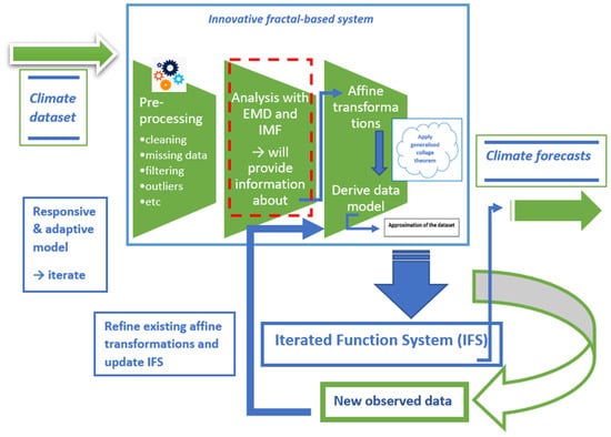
Figure 1. Conceptual architecture of the Rapid Adaptive Climate Change (RACC) framework. Adapted from [29].

Within RACC, datasets from atmospheric and hydrospheric domains are processed in parallel layers that preserve abstraction at the variable level while allowing interconnectivity for downstream analysis and forecasting tasks. The framework integrates datasets from both domains to explore dynamic cross-domain relationships—particularly thermal feedback mechanisms between hydrospheric processes, including cryospheric change, and trends in global mean atmospheric temperature. At the core of our approach lies EMD and its variants, which are employed to extract dependent components (IMFs) from each environmental time series. Unlike traditional EMD applications that rely directly on IMFs for forecasting (e.g., [31]), our framework utilises these components to inform the construction of an iterated function system (IFS)—a methodological extension aimed at addressing the key limitations of EMD. These include the unpredictable number of IMFs generated and the difficulty in attributing them to specific periodic sources [32].

By integrating a diverse range of environmental data streams within a unified, iterative model structure, RACC aims to produce a comparative forecasting platform that evolves with changing inputs without reliance on large-scale data assimilation.

Our approach is vital, offering a responsive way to model local climate variations, benefiting local policymaking and citizen scientists’ understanding of climate-related local environmental changes. This fosters a deeper comprehension of climate change and encourages behavioural changes in local populations.

3. Our Empirical-Based Contribution

In earth science and especially in the marine environment, the recorded time series are often nonlinear and nonstationary and interact with each other. To accommodate the variety of data generated by nonlinear and nonstationary processes, Huang et al. developed EMD as an adaptive time series analysis method [30] which has been applied to different fields such as the ocean, the atmosphere, signal processing, mechanical engineering, climate studies, earthquakes, and biomedical studies. Their paper has reached nearly 30,000 citations so far.

EMD Principle

The key part of EMD is that any complicated dataset can be decomposed with the method into a finite and small number of IMFs [30]. These represent different scales of the original time series and physically meaningful modes. An IMF is defined as a function with the same number of extrema and zero-crossings. It also has symmetric upper and lower envelopes defined by local maxima and minima, respectively.

Indeed, EMD divides the time series into a series of modes and allows each mode to have a time-dependent frequency and amplitude. In contrast to almost all the previous methods, EMD works directly in temporal space, rather than in the corresponding frequency space. Due to a dyadic filter bank property of the EMD algorithm [33,34,35], usually, in practice, the number of IMF modes is less than ${\log }_{2}N$, where $N$ is the number of observations.

Ensemble empirical mode decomposition (EEMD) [36] and complete ensemble empirical mode decomposition (CEEMD) [37] are advanced versions of EMD, designed to mitigate EMD’s limitations like mode mixing and modal aliasing. They inject stochasticity into the decomposition process, improving robustness and reliability. In CEEMDAN, the original signal is iteratively decomposed into IMFs with adaptive noise. It is particularly effective when dealing with signals that exhibit non-linear and non-stationary characteristics. The technique was developed to address some of the limitations of EMD when dealing with noisy signals.

It is noteworthy to mention recent developments in algorithms such as sparse variational mode decomposition (SVMD) and its versatile applications in various fields. Notably, studies like [38] have showcased the potential of SVMD to enhance adaptive feature extraction techniques. Such advancements have the potential to complement the EMD framework, enhancing its adaptability and effectiveness in capturing the complex signal dynamic.

4. A Variable-Centric Approach to IMF Upper Bound Estimation

This section presents an empirical enhancement to the traditional EMD technique and its variants, as applied within the RACC framework. The relevant component in the model architecture is illustrated in Figure 1 (indicated by the red dashed line). Building on the initial work outlined in [29], we propose a refined upper bound for estimating the number of IMFs required for signal decomposition.

Conventionally, the number of IMFs is heuristically bounded by ${\log }_{2}N$, where $N$ is the number of observations [30]. While effective for long and information-rich datasets, this approach can lead to over-decomposition, reduced physical interpretability, and unnecessary computational expense when applied to sparse or regional environmental datasets. However, empirical analysis conducted across multiple environmental datasets suggests that the effective number of energetically significant IMFs saturates well below this bound once all dominant variable interactions are captured. Motivated by this observation, our investigation suggests a more efficient estimation rule, based on the dimensionality of the data rather than its length. Specifically, we propose the following empirical formula:

$$nf=nv+\mathrm{r}\mathrm{o}\mathrm{u}\mathrm{n}\mathrm{d}\left({\displaystyle \frac{nv}{3}}\right)$$

(1)

Here, $nf$ denotes the estimated number of IMFs, and $nv$ refers to the number of input variables. These variables represent distinct physical measurements, such as air temperature, humidity, rainfall, and barometric pressure. For time series data, we consistently include an additional temporal variable, resulting in a five-variable model in our case. The proposed upper bound formula is empirically derived from repeated decomposition experiments across multiple environmental datasets and is conceptually motivated by the hypothesis that signal complexity scales with the number of interacting variables, rather than data length. While not derived from first principles, the formulation reflects the observed saturation in the explained variance beyond a small number of IMFs once all principal variable interactions are captured and the principal degrees of freedom of the system are resolved. Under this assumption, each IMF captures either a dominant variable-specific oscillation or an interaction-driven mode, and additional IMFs beyond this point tend to fragment existing dynamics without contributing meaningful explanatory power. This perspective provides a pragmatic and physically interpretable criterion for constraining EMD-based decompositions in adaptive climate modelling.

To illustrate, consider a dataset with hourly readings over six months ($N=4344$). The conventional approach would suggest up to 12 IMFs (${\log }_2\left(4344\right)\approx 12$). Our model, by contrast, yields a significantly lower estimate of $nf=6$ IMFs for five variables. Importantly, this value remains unchanged when extending the time window (e.g., from six months to a full year), as it is governed by the number of variables rather than data length.

This result stems from the hypothesis that the complexity of the decomposed signal is more tightly linked to the interactions among variables than to the volume of data alone. We posit that for every three spatial variables, an additional function is required to capture temporal or interaction-based dynamics that are not explicitly represented in the individual IMFs. Although not a strict mathematical analogy, this conceptual model accounts for latent relationships that emerge through the integration of environmental signals over time.

The principal contribution of this work is the introduction of a variable-centric empirical upper bound for IMF estimation, which departs fundamentally from conventional observation-length-based heuristics. Unlike the existing EMD-based frameworks that treat IMF count as an emergent by-product of the algorithm, our approach explicitly links decomposition complexity to the number of interacting environmental variables. This results in improved interpretability, reduced redundancy, and enhanced suitability for sparse and regional datasets.

5. Adaptive Forecasting from Sparse Climate Datasets: A Case Study in the Minas Passage

This case study is intended not as an isolated demonstration but as an illustrative example of how the proposed IMF constraint supports adaptive modelling under data sparsity, a common limitation in regional climate studies. The Minas Passage, located in the inner Bay of Fundy in Nova Scotia, Canada, presents a challenging but informative test case due to the sparsity of available data. While sparse datasets are often treated as a limiting factor, our approach demonstrates that they can be effectively leveraged to construct reproducible and adaptive forecasting models in climate science. The objective of this case study is therefore not to maximise predictive accuracy in isolation, but to demonstrate how the proposed variable-centric IMF constraint supports reproducible and adaptive modelling under data-limited conditions. Crucially, our method avoids the need for the high computational overhead that is typically associated with recomputing interactions across large-scale datasets. Instead, we construct inverse problems to uncover latent relationships between climate components, without requiring fixed lag assumptions.

In this context, we model the interaction between the thermal capacities of the hydrosphere and the atmosphere through transformations discovered in the data. By employing affine transformations and probabilistic associations, we abstract the data into a reduced but informative structure that preserves the key characteristics of the climate system. This abstraction facilitates the development of iterative, probabilistic forecasting models akin to those proposed by [23].

Our framework enables continuous adaptation to new data inputs, accommodating dynamic changes such as altered lag relationships between environmental components—e.g., the influence of accelerated ice melt on the hydrosphere’s heat storage capacity. This adaptive capacity is particularly valuable in regional climate modelling scenarios where data may be limited or evolving over time. Within this context, the case study serves as a practical demonstration of how constraining the number of IMFs does not hinder the identification of dominant physical cycles but instead enhances the interpretability and stability.

6. Simulation Results

In this section, we present the data and statistical results from the experiments, running CEEMDAN with the new metric to derive the number of IMFs required. Figure 2 shows the Minas Passage data for the first six months of 2015 as an illustration. Our analysis incorporates various variables, including air temperature, barometric pressure, humidity, and rainfall.

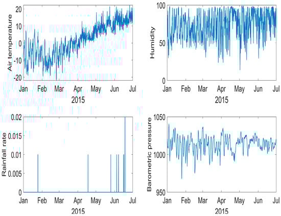
Figure 2. Data from the first six months of 2015 for various variables, including air temperature, barometric pressure, humidity, and rainfall. These variables constitute the multivariate input to the EMD-based analysis and illustrate the non-stationary and heterogeneous nature of the dataset used to evaluate the proposed variable-centric IMF constraint.

6.1. EMD-Based Results

The following simulations demonstrate the results of applying CEEMDAN to the data without restricting the maximum number of IMFs, in accordance with the formula given above in Equation (1). Figure 3 shows the CEEMDAN decomposition of the barometric pressure. Nine IMF modes are extracted, plus the residual component. The timescale is increasing with the number of the IMF mode: the first IMF thus corresponds to the highest frequency. The residual from the EMD algorithms has been recognised as the trend of the given data [39,40,41]. Among the IMFs identified in Figure 3, six were found to be the predominant modes within the signal, collectively contributing to over 97% of the total variability, as measured by variance. Likewise, when we conducted CEEMDAN decomposition on temperature and rainfall data, the six most energetically significant IMFs accounted for over 94% and almost 96% of the total variability, respectively. These consistent findings provide strong validation for our empirical approach, which involves constraining the maximum number of IMFs, as specified in Equation (1).

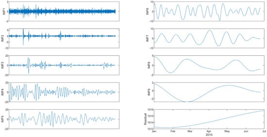
Figure 3. CEEMDAN decomposition of barometric pressure for the first six months of 2015. Although nine IMFs and a residual are extracted when no constraint is applied, the first six IMFs account for more than 97% of the total variance. This result demonstrates that the dominant dynamics of the signal are captured within a limited number of modes, providing empirical support for the proposed variable-centric upper bound on the number of IMFs.

A qualitative comparison between the unconstrained CEEMDAN decomposition and the proposed variable-constrained approach highlights several advantages. While unconstrained CEEMDAN produced a larger number of IMFs, a substantial proportion of the total variance was consistently captured by a smaller subset of dominant modes. By constraining the number of IMFs, the proposed method reduces redundancy, improves interpretability, and lowers computational overhead without compromising the identification of key physical cycles. These observations indicate that the proposed approach offers a more parsimonious and efficient representation compared to traditional EMD-based decompositions.

6.2. Significance of IMFs

We argue that the remaining characteristic in the signal that is not captured by an IMF (excluding the residual) corresponds to the evolving relationships between the signal’s components over time. Further decomposition risks fragmenting these dynamic interactions into isolated features, which we deliberately avoid in order to maintain meaningful interdependencies within the modes. Although the residual typically carries a greater magnitude than each individual IMF, together they encapsulate the essential characteristics of the original signal. This balance is vital, as it lays the foundation for advancing a probabilistic modelling approach, which remains an important focus of our ongoing research.

Not all extracted IMFs can be directly attributed to distinct physical processes. In this study, the relative significance of IMFs is assessed primarily through their contribution to total variance and their consistency across variables and datasets. Dominant IMFs that account for the majority of the signal energy are interpreted as physically meaningful modes, while lower-energy components are treated as representing secondary interactions or stochastic influences. In particular, the lower-frequency IMFs are likely to be representative of periodic variations such as the lunar cycle. Furthermore, some of the IMFs will represent frequencies which result from interactions of other cycles and therefore do not have any direct physical meaning. This variance-based criterion provides a pragmatic proxy for statistical significance in the context of sparse environmental datasets. Formal hypothesis-based significance testing of individual IMFs constitutes an important extension of this work and will be incorporated in future developments of the framework. This distinction is illustrated in the CEEMDAN analysis of pressure data from the Minas Passage, where specific IMFs correspond to identifiable periodic components while others capture mixed or emergent frequencies. Here is an illustrative breakdown:

• Higher-frequency IMFs (e.g., IMF 1, IMF 2): Likely capture high-frequency fluctuations due to turbulence, small-scale eddies, or high-frequency tidal constituents.
• Medium-frequency IMFs (e.g., IMF 4, IMF 6): These could correspond to diurnal and semi-diurnal tidal components, which are dominant in regions with significant tidal influence like the Minas Passage.
• Lower-frequency IMFs (e.g., IMF 8, IMF 9): These IMFs may represent longer-period tidal components, such as the monthly tidal variations (e.g., lunar synodic month) and meteorological influences. A “monthly wave” would be reflected in these lower frequency IMFs.

6.3. IMF Results

We also calculated the main periods for each IMF variable. Several distinct waves were identified within the barometric pressure decomposition, including semi-diurnal and diurnal oscillations, 5-day and 9-day cycles in the Minas Passage, and monthly and seasonal waves. This observation underscores that the main periodic cycles that are inherent to the signal are successfully identified through the EMD process. Notably, our new empirical measure, which limits the number of IMFs to just six in this instance, does not impede the identification process of these cycles. Assuming $h_j^i\left(t\right)$ is jth IMF of timeseries $x_i\left(t\right)$, we find the mean period $T_j^i(t)$ of each $h_j^i(t)$, either by calculating the local extrema points and zero crossing points, i.e., $T_j^i\left(t\right)=4\times {\displaystyle \frac{data length}{{Nbr}_{max}+{Nbr}_{min}+{Nbr}_0}}$ [42] or by considering the Fourier energy weighted mean frequency, i.e., $T_j^i\left(t\right)={\displaystyle \frac{\int {\left|X_j^i(f)\right|}^{2}df}{\int {f\left|X_j^i(f)\right|}^{2}df}}$, where $X_j^i(f)$ is the Fourier power spectrum of each IMF mode.

We investigated the variances for each IMF per input variable. The humidity exhibited the highest variance among them all. Given the low rainfall, the predominant interaction will be the air temperature combined with the barometric pressure, causing changes in humidity. Nevertheless, our approach demonstrates that the new empirical measure identifies relationships between the variables at a variance level that reflects the expected change throughout the year.

We extended the application of our proposed methodology to multiple datasets to further demonstrate its effectiveness and generalisability, showcasing the robustness of our approach across diverse scenarios. For example, we employed our approach to analyse five time series data, encompassing temperature, turbidity, salinity, density, and chlorophyll levels in the Gascoyne Inlet. The authors in [32] initially applied EMD to these datasets. In line with our approach, which considers $nv$ = 6 variables, including time, we proceeded with CEEMDAN decomposition, setting $nf=nv+\mathrm{r}\mathrm{o}\mathrm{u}\mathrm{n}\mathrm{d}\left({\displaystyle \frac{nv}{3}}\right)=8$, as opposed to the 13 IMFs plus the residual identified in [32]. For the chlorophyll, the analysis of the eight most significant IMFs accounted for almost 97% of the total energy, thereby affirming the soundness and validity of our approach.

While the present study focuses on oceanic and coastal environmental datasets, the proposed variable-centric IMF upper bound is not intrinsically domain-specific. Its formulation depends on the dimensionality of the input variables rather than the physical setting of the system. Terrestrial climate datasets often exhibit comparable multivariate structure and non-stationary behaviour, suggesting that the proposed approach is directly transferable. A systematic evaluation using terrestrial climate variables (e.g., land surface temperature, soil moisture, and precipitation) is therefore identified as an important direction for future work and will be pursued in subsequent studies.

7. Conclusions

In summary, our study presents a pioneering approach with significant implications for climate modelling:

(1) Methodological innovation: Our introduction of an empirical upper bound formula for determining the necessary IMFs within EMD-based decompositions represents a crucial innovation. This formula, grounded in the number of variables rather than observations, effectively addresses a key limitation of conventional EMD methods.

(2) Enhanced data-centric approach: By shifting the focus towards a variable-centric methodology, our approach has the potential to revolutionise climate analysis, especially when dealing with smaller datasets. This adaptability offers a pathway to a deeper understanding of complex systems like climate variations.

(3) Complementary to established models: It is essential to emphasise that our approach does not seek to replace the existing climate models but rather complements them. By augmenting prevailing mathematical frameworks, our methodology empowers us to make more accurate short-term climate predictions, thus enabling informed and impactful policy decisions. Collectively, these contributions mark a significant step forward in the realm of climate modelling. Our innovative methodology, while rooted in empirical mode-based techniques, offers a fresh perspective that holds promise for more adaptable, responsive, and precise climate predictions.

Further research will include applying our innovation to a wider variety of datasets to establish the robustness of our algorithm across more domains.

References

- Chevuturi, A.; Turner, A.G.; Woolnough, S.J.; Martin, G.M.; MacLachlan, C. Indian summer monsoon onset forecast skill in the UK Met Office initialized coupled seasonal forecasting system (GloSea5-GC2). Clim. Dyn. 2019, 52, 6599–6617. [Google Scholar] [CrossRef]
- Brönnimann, S. Impact of El Niño–southern oscillation on European climate. Rev. Geophys. 2007, 45. [Google Scholar] [CrossRef]
- IPCC. Climate Change 2022: Mitigation of Climate Change. Contribution of Working Group III to the Sixth Assessment Report of the Intergovernmental Panel on Climate Change; Shukla, P.R., Skea, J., Slade, R., Al Khourdajie, A., van Diemen, R., McCollum, D., Pathak, M., Some, S., Vyas, P., Fradera, R., et al., Eds.; Cambridge University Press: Cambridge, UK; New York, NY, USA, 2022. [Google Scholar] [CrossRef]
- Ossó, A.; Allan, R.; Hawkins, E.; Shaffrey, L.; Maraun, D. Emerging New Climate Extremes Over Europe. Clim. Dyn. 2022, 58, 487–501. [Google Scholar] [CrossRef]
- Stott, P. How climate change affects extreme weather events. Science 2016, 352, 1517–1518. [Google Scholar] [CrossRef]
- Knutti, R.; Sedláček, J. Robustness and uncertainties in the new CMIP5 climate model projections. Nat. Clim. Change 2013, 3, 369–373. [Google Scholar] [CrossRef]
- Vavrus, S.J.; Notaro, M.; Lorenz, D.J. Interpreting climate model projections of extreme weather events. Weather Clim. Extrem. 2015, 10, 10–28. [Google Scholar] [CrossRef]
- Schewe, J.; Gosling, S.N.; Reyer, C.; Zhao, F.; Ciais, P.; Elliott, J.; Francois, L.; Huber, V.; Lotze, H.K.; Seneviratne, S.I.; et al. State-of-the-art global models underestimate impacts from climate extremes. Nat. Commun. 2019, 10, 1005. [Google Scholar] [CrossRef]
- Hamill, T.M.; Juras, J. Measuring forecast skill: Is it real skill or is it the varying climatology? Q. J. R. Meteorol. Soc. 2006, 132, 2905–2923. [Google Scholar] [CrossRef]
- Stevens, B.; Bony, S. What are climate models missing? Science 2013, 340, 1053–1054. [Google Scholar] [CrossRef] [PubMed]
- Paeth, H.; Scholten, A.; Friederichs, P.; Hense, A. Uncertainties in climate change prediction: El Niño-Southern Oscillation and monsoons. Glob. Planet. Change 2008, 60, 265–288. [Google Scholar] [CrossRef]
- Déqué, M.; Somot, S.; Sanchez-Gomez, E.; Goodess, C.M.; Jacob, D.; Lenderink, G.; Christensen, O.B. The Spread Amongst ENSEMBLES Regional Scenarios: Regional Climate Models, Driving General Circulation Models and Interannual Variability. Clim. Dyn. 2012, 38, 951–964. [Google Scholar] [CrossRef]
- Beniston, M.; Stephenson, D.B.; Christensen, O.B.; Ferro, C.A.; Frei, C.; Goyette, S.; Halsnaes, K.; Holt, T.; Jylhä, K.; Koffi, B.; et al. Future extreme events in European climate: An exploration of regional climate model projections. Clim. Change 2007, 81, 71–95. [Google Scholar] [CrossRef]
- Smith, D.M.; Eade, R.; Dunstone, N.J.; Fereday, D.; Murphy, J.M.; Pohlmann, H.; Scaife, A.A. Skilful multi-year predictions of Atlantic hurricane frequency. Nat. Geosci. 2010, 3, 846–849. [Google Scholar] [CrossRef]
- Kumar, A.; Peng, P.; Chen, M. Is there a relationship between potential and actual skill? Mon. Weather Rev. 2014, 142, 2220–2227. [Google Scholar] [CrossRef]
- Teutschbein, C.; Seibert, J. Bias correction of regional climate model simulations for hydrological climate-change impact studies: Review and evaluation of different methods. J. Hydrol. 2012, 456–457, 12–29. [Google Scholar] [CrossRef]
- Li, W.; Duan, Q.; Miao, C.; Ye, A.; Gong, W.; Di, Z. A review on statistical postprocessing methods for hydrometeorological ensemble forecasting. Water 2017, 4, e1246. [Google Scholar] [CrossRef]
- Zhao, T.; Bennett, J.C.; Wang, Q.J.; Schepen, A.; Wood, A.W.; Robertson, D.E.; Ramos, M.H. How suitable is quantile mapping for postprocessing GCM precipitation forecasts? J. Clim. 2017, 30, 3185–3196. [Google Scholar] [CrossRef]
- Vidale, P.L.; Lüthi, D.; Frei, C.; Seneviratne, S.I.; Schär, C. Predictability and uncertainty in a regional climate model. J. Geophys. Res. 2003, 108, 4586. [Google Scholar] [CrossRef]
- Xie, S.P.; Deser, C.; Vecchi, G.A.; Collins, M.; Delworth, T.L.; Hall, A.; Hawkins, E.; Johnson, N.C.; Cassou, C.; Giannini, A.; et al. Towards predictive understanding of regional climate change. Nat. Clim. Change 2015, 5, 921–930. [Google Scholar] [CrossRef]
- Kbaier Ben Ismail, D.; Lazure, P.; Puillat, I. Advanced Spectral Analysis and Cross Correlation Based on the Empirical Mode Decomposition: Application to the Environmental Time Series. IEEE Geosci. Remote Sens. Lett. 2015, 12, 1968–1971. [Google Scholar] [CrossRef]
- Kunze, H.; Torre, D.L.; Levere, K.; Galán, M.R. Inverse Problems via the (Generalized Collage Theorem) for Vector-Valued Lax-Milgram-Based Variational Problems. Mathematical Problems in Engineering. Math. Probl. Eng. 2015, 2015, 764643. [Google Scholar] [CrossRef]
- Sévellec, F.; Drijfhout, S.S. A novel probabilistic forecast system predicting anomalously warm 2018–2022 reinforcing the long-term global warming trend. Nat. Commun. 2018, 9, 3024. [Google Scholar]
- Rasheed, A.; Veluvolu, K.C. Respiratory Motion Prediction with Empirical Mode Decomposition-Based Random Vector Functional Link. Mathematics 2024, 12, 588. [Google Scholar] [CrossRef]
- Yin, C.; Wei, N.; Wu, J.; Ruan, C.; Luo, X.; Zeng, F. An Empirical Mode Decomposition-Based Hybrid Model for Sub-Hourly Load Forecasting. Energies 2024, 17, 307. [Google Scholar] [CrossRef]
- Deb, M.; Dhar, M.K.; Elangovan, P.; Gopalakrishnan, K.; Sood, D.; Sethi, A.; Afroze, S.; Bansal, S.; Goudel, A.; Parikh, C.; et al. Empirical Mode Decomposition-Based Deep Learning Model Development for Medical Imaging: Feasibility Study for Gastrointestinal Endoscopic Image Classification. J. Imaging 2026, 12, 4. [Google Scholar] [CrossRef]
- Yao, S.; Zhu, H.; Zhou, X.; Peng, T.; Zhang, J. LSTM Model Combined with Rolling Empirical Mode Decomposition and Sample Entropy Reconstruction for Short-Term Wind Speed Forecasting. Processes 2025, 13, 819. [Google Scholar] [CrossRef]
- Chang, C.-W.; Huang, W.-C. Application of Empirical Mode Decomposition to Land Surface Temperature Projection Under a Changing Climate. Water 2025, 17, 2204. [Google Scholar] [CrossRef]
- Kenny, I.; Kbaier, D. Rapid Adaptive Climate Change Model: Application of a Probabilistic Centred Approach to the Minas Passage Bay of Fundy datasets. In Proceedings of the OCEANS 2022, Hampton Roads, VA, USA, 17–20 October 2022; pp. 1–5. [Google Scholar] [CrossRef]
- Huang, N.E.; Shen, Z.; Long, S.R.; Wu, M.C.; Shih, H.H.; Zheng, Q.; Yen, N.C.; Tung, C.C.; Liu, H.H. The Empirical Mode Decomposition and the Hilbert Spectrum for Nonlinear and Non-stationary Time Series Analysis. Proc. R. Soc. Lond. Ser. A Math. Phys. Eng. Sci. 1998, 454, 903–995. [Google Scholar]
- Le, J.A.; El-Askary, H.M.; Allali, M.; Sayed, E.; Sweliem, H.; Piechota, T.C.; Struppa, D.C. Characterizing El Niño-Southern Oscillation Effects on the Blue Nile Yield and the Nile River Basin Precipitation Using Empirical Mode Decomposition. Earth Syst. Environ. 2020, 4, 699–711. [Google Scholar] [CrossRef]
- Kbaier, D. Advanced statistical analysis of environmental data in the Gascoyne Inlet. In Proceedings of the MTS/IEEE OCEANS’ 2021: San Diego—Porto, San Diego, CA, USA, 20–23 September 2021. [Google Scholar]
- Flandrin, P.; Rilling, G.; Goncalves, P. Empirical mode decomposition as a filter bank. IEEE Signal Process. Lett. 2004, 11, 112–114. [Google Scholar] [CrossRef]
- Huang, Y.; Schmitt, F.; Lu, Z.; Liu, Y. An amplitude-frequency study of turbulent scaling intermittency using Empirical Mode Decomposition and Hilbert Spectral Analysis. Europhys. Lett. 2008, 84, 40010. [Google Scholar] [CrossRef]
- Wu, Z.; Huang, N.E. A study of the characteristics of white noise using the empirical mode decomposition method. Proc. R. Soc. Lond. A 2004, 460, 1597–1611. [Google Scholar] [CrossRef]
- Wu, Z.; Huang, N.E. Ensemble empirical mode decomposition: A noise-assisted data analysis Method. AADA Adv. Adapt. Data Anal. 2009, 1, 1–41. [Google Scholar]
- Torres, M.E.; Colominas, M.A.; Schlotthauer, G.; Flandrin, P. A complete ensemble empirical mode decomposition with adaptive noise. In Proceedings of the 2011 IEEE International Conference on Acoustics, Speech, and Signal Processing, Prague, Czech Republic, 22–27 May 2011; pp. 4144–4147. [Google Scholar] [CrossRef]
- Li, Y.; Tang, B.; Jiao, S. SO-slope entropy coupled with SVMD: A novel adaptive feature extraction method for ship-radiated noise. Ocean Eng. 2023, 280, 114677. [Google Scholar] [CrossRef]
- Kbaier Ben Ismail, D.; Lazure, P.; Puillat, I. Statistical properties and time-frequency analysis of temperature, salinity and turbidity measured by the MAREL Carnot station in the coastal waters of Boulogne-sur-Mer (France). J. Mar. Syst. 2016, 162, 137–153. [Google Scholar] [CrossRef]
- Moghtaderi, A.; Borgnat, P.; Flandrin, P. Trend filtering: Empirical mode decompositions versus l1 and Hodrick–Prescott. Adv. Adapt. Data Anal. 2011, 3, 41–61. [Google Scholar] [CrossRef]
- Wu, Z.; Huang, N.; Long, S.; Peng, C. On the trend, detrending, and variability of nonlinear and nonstationary time series. Proc. Natl. Acad. Sci. USA 2007, 104, 14889. [Google Scholar] [CrossRef]
- Huang, Y.; Schmitt, F. Time dependent intrinsic correlation analysis of temperature and dissolved oxygen time series using empirical mode decomposition. J. Mar. Syst. 2014, 130, 90–100. [Google Scholar] [CrossRef]
Disclaimer/Publisher’s Note: The statements, opinions and data contained in all publications are solely those of the individual author(s) and contributor(s) and not of MDPI and/or the editor(s). MDPI and/or the editor(s) disclaim responsibility for any injury to people or property resulting from any ideas, methods, instructions or products referred to in the content. |
© 2026 by the authors. Licensee MDPI, Basel, Switzerland. This article is an open access article distributed under the terms and conditions of the Creative Commons Attribution (CC BY) license.