Abstract
Accurate simulation of extreme precipitation events is crucial for managing climate-vulnerable sectors in Southern Africa, as such events directly impact agriculture, water resources, and disaster preparedness. However, global climate models frequently struggle to capture these phenomena, which limits their practical applicability. This study investigates the effectiveness of three bias correction techniques—scaled distribution mapping (SDM), quantile distribution mapping (QDM), and QDM with a focus on precipitation above and below the 95th percentile (QDM95)—and the daily precipitation outputs from 11 Coupled Model Intercomparison Project Phase 6 (CMIP6) models. The Climate Hazards Group Infrared Precipitation with Stations (CHIRPS) dataset was served as a reference. The bias-corrected and native models were evaluated against three observational datasets—the CHIRPS, Multi-Source Weighted Ensemble Precipitation (MSWEP), and Global Precipitation Climatology Center (GPCC) datasets—for the period of 1982–2014, focusing on the December-January-February season. The ability of the models to generate eight extreme precipitation indices developed by the Expert Team on Climate Change Detection and Indices (ETCCDI) was evaluated. The results show that the native and bias-corrected models captured similar spatial patterns of extreme precipitation, but there were significant changes in the amount of extreme precipitation episodes. While bias correction generally improved the spatial representation of extreme precipitation, its effectiveness varied depending on the reference dataset used, particularly for the maximum one-day precipitation (Rx1day), consecutive wet days (CWD), consecutive dry days (CDD), extremely wet days (R95p), and simple daily intensity index (SDII). In contrast, the total rain days (RR1), heavy precipitation days (R10mm), and extremely heavy precipitation days (R20mm) showed consistent improvement across all observations. All three bias correction techniques enhanced the accuracy of the models across all extreme indices, as demonstrated by higher pattern correlation coefficients, improved Taylor skill scores (TSSs), reduced root mean square errors, and fewer biases. The ranking of models using the comprehensive rating index (CRI) indicates that no single model consistently outperformed the others across all bias-corrected techniques relative to the CHIRPS, GPCC, and MSWEP datasets. Among the three bias correction methods, SDM and QDM95 outperformed QDM for a variety of criteria. Among the bias-corrected strategies, the best-performing models were EC-Earth3-Veg, EC-Earth3, MRI-ESM2, and the multi-model ensemble (MME). These findings demonstrate the efficiency of bias correction in improving the modeling of precipitation extremes in Southern Africa, ultimately boosting climate impact assessments.
Keywords:
bias correction; precipitation extremes; CHIRPS; CMIP6 models; GPCC; MSWEP; Southern Africa 1. Introduction
The impacts of extreme weather and climate events on society and the environment have become increasingly severe in recent years, raising concerns about ecosystems and societal vulnerability [1,2]. For instance, extreme precipitation events have significantly affected human populations, ecosystems, and infrastructure. This has led to increased flooding, landslides, and erosion, resulting in property damage, loss of life, and displacement of communities [3]. The Sixth Assessment Report (AR6) of the Intergovernmental Panel on Climate Change (IPCC) highlights the disproportionate impacts of climate change on societies with limited adaptive capacities [4]. The Southern African region is particularly vulnerable due to a combination of a low adaptation capacity and limited understanding of climate variability. Recent extreme events driven by climate change have exacerbated water scarcity, droughts, disrupted ecosystems, jeopardized food security, destroyed infrastructure, and caused loss of life [5,6]. For example, the 2015–2016 drought led to widespread crop failure and severe food insecurity. Similarly, heavy precipitation events associated with tropical cyclones have resulted in extreme flooding, leading to deaths, displacement, and infrastructure damage [7,8]. As recently as 19 February 2025, Gaborone, Botswana experienced severe flooding after several days of heavy rain caused the Gaborone Dam to overflow. Many areas in Botswana recorded rainfall amounts ranging from 150 mm to over 200 mm within a 24-h period several times leading up to the severe flooding. This disaster affected over 5000 people, displaced nearly 2000 individuals and households, and resulted in the deaths of 9 people (https://www.voanews.com/a/deadly-floods-in-botswana-kill-9-nearly-2-000-people-evacuated/7986895.html, accessed on 19 February 2025).
As a result, understanding the spatiotemporal patterns of extreme precipitation is critical for assessing water resource availability, ecosystem dynamics, and economic development and managing disaster-related risks [9,10]. Changes in extreme precipitation patterns are also crucial for evaluating climate models and improving extreme weather forecasts [3,11]. Numerous studies have shown that climate models often underestimate the intensity and overestimate the frequency of extreme precipitation patterns [12,13,14]. However, many studies do not apply bias correction methods, compromising their accuracy. Global climate models (GCMs) are critical tools for studying climate extremes at global and regional scales, but they often struggle to simulate extreme precipitation events accurately due to their coarse-gridded resolution and inherent model biases [15,16]. This limitation leads to significant biases that reduce their usefulness for regional and local impact studies, such as hydrological, ecological, and agricultural modeling [17,18]. Bias correction techniques are therefore essential to improving GCM performance, particularly in accurately capturing extreme precipitation events.
Several bias correction methods have been developed to address these model biases, with distribution-based approaches proving particularly effective for correcting precipitation biases [19,20,21]. For instance, Gumindoga et al. [22] found that quantile mapping based on empirical distributions produced the best results for satellite precipitation estimates. Similar findings were reported by Tabari et al. [20] and Chen et al. [23], who concluded that quantile mapping on a gamma distribution yielded favorable outcomes for precipitation bias correction. Studies conducted across Africa, such as those by Ayugi et al. [24], Hamadalnel et al. [25], and Jaiswal et al. [21], demonstrated improvements in model accuracy using similar quantile mapping techniques.
Many studies have investigated extreme precipitation variability in Southern Africa using CMIP5 and CMIP6 [26,27,28,29]. For instance, Bellprat et al. [26] examined wet and dry seasons using CMIP5 data, revealing that despite a general drying trend, heavy moisture flux could increase the frequency of heavy precipitation events. Sian et al. [27] compared CMIP6 to evaluate the impact of the bias correction method on extreme precipitation, uncovering a notable drying trend in spatiotemporal projections during wet and dry seasons. While they focused primarily on future projections, they did not delve into a detailed comparison of simulated historical extreme precipitation. Samuel et al. [28] utilized the Bias Correction with Spatial Disaggregation (BCSD) technique to enhance the accuracy of CMIP6 models for assessing mean and extreme precipitation over Sub-Saharan Africa, employing the Global Meteorological Forcing Dataset (GMFD) as a reference. Their analysis, however, solely tested the performance of the quantile mapping bias correction method, which is used by BCSD. Furthermore, previous studies have thoroughly explored excessive precipitation in portions of Southern Africa, such as South Africa, the Namib Desert, and southeastern Africa [8,30,31,32], which has significantly contributed to the understanding of its effects in these regions. However, these studies did not use bias-corrected data. While these studies examined the reliability of bias-corrected climate models (e.g., CMIP6, CMIP5, and CORDEX) in simulating high extreme precipitation levels at both global and regional scales—especially in areas with complex climate zones and varied topography—it appears that their effectiveness in accurately capturing high extreme precipitation indices in Southern Africa has not been thoroughly investigated. To address these gaps, this study evaluates the performance of eleven CMIP6 models using three bias correction techniques to reproduce observed extreme precipitation during the peak rainy season (from December to February (DJF)). This study builds upon our previous research (Addisuu et al. [33]), which focused on the spatiotemporal characterization of native and bias-corrected precipitation relative to observational data. In this paper, we expand our previous analysis to evaluate how bias correction improves the representation of precipitation extremes in CMIP6 models compared with three observational datasets.
The structure of this paper is as follows. Section 2 outlines the datasets and methodologies employed, including the calculation of extreme precipitation indices. Section 3 presents the findings from comparing bias-corrected and uncorrected simulations against observational data. Finally, Section 4 summarizes the key findings regarding the ability of CMIP6 models to simulate extreme precipitation indices and the improvements achieved through bias correction, and it identifies the most effective bias correction technique.
2. Study Area, Data, and Methods
2.1. The Study Area
This study was undertaken in Southern Africa, covering an extensive range of coordinates from approximately 9 to 35 degrees south latitude and from 11 to 51 degrees east longitude (Figure 1). A large drainage basin within this region with coastlines from the Atlantic Ocean to the Indian Ocean reaches Cape Agulhas. Eleven countries, including the island nation of Madagascar, namely Zimbabwe, Malawi, Botswana, Angola, Zambia, Namibia, Mozambique, Lesotho, Eswatini, and South Africa, are encompassed within this geographical area.
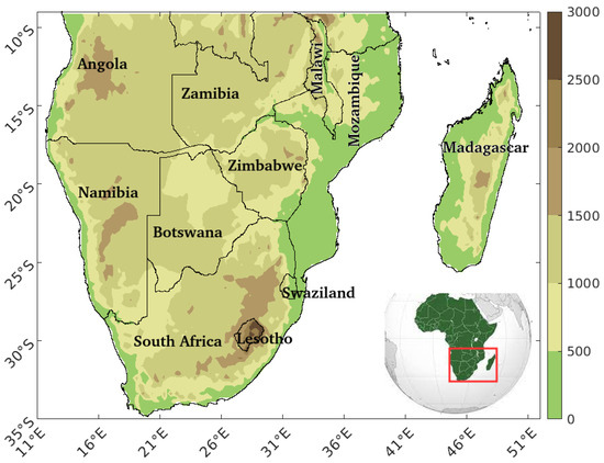
Figure 1.
The red box shows the location of the study area in Africa. The zoomed inset illustrates the elevation (in meters) and the borders of the countries within the study area. The surface elevation data were obtained from ETOPO2 [34].
2.2. Data and Methods
2.2.1. Observational Data
To ensure robust and reliable results, three observational datasets were carefully selected for this study, following recommendations from a previous investigation in Sub-Saharan Africa [28]. This previous work emphasized the importance of using multiple high-resolution datasets, such as Climate Hazards Group Infrared Precipitation with Station (CHIRPS) and Multi-Source Weighted Ensemble Precipitation (MSWEP), to address uncertainties in observational data and enhance the reliability of bias-corrected projections. Because of its proven accuracy over Southern Africa and its capacity to overcome the spatiotemporal limitations of rain gauges, the CHIRPS dataset—which offers a thorough daily precipitation record from 1982 to 2014 with a high spatial resolution of 0.25°—was selected as the reference in the bias correction and as one of the sets of observational data in the evaluation of the native model and bias-corrected precipitation for this study [35]. Similarly, the MSWEP dataset utilizes spatial resolutions of , with temporal daily precipitation data available from 1982 to 2014. MSWEP incorporates satellite imagery, ground observations, and reanalysis for comprehensive precipitation data, providing a robust global picture [36]. MSWEP’s superior performance in daily precipitation estimates compared with other options [37], coupled with its high spatial resolution, made it the ideal choice as one of the observational datasets in this study. Furthermore, the Global Precipitation Climatology Center (GPCC) Full Data Daily Version 2020 dataset was utilized as another observational dataset against which the native and bias-corrected models were assessed. Covering the period from 1982 to 2014 with a spatial resolution of , GPCC ensured extensive observational coverage, enhancing the reliability of the analysis [38].
2.2.2. CMIP6 Climate Models
This study evaluated the effectiveness of bias correction techniques in capturing extreme precipitation characteristics using 11 general circulation models (GCMs) from the CMIP6 dataset. These models were the same as those employed by Addisuu et al. (2025) (the companion paper, Part I), which focused on assessing improvements in the spatiotemporal characteristics of precipitation through bias correction. By maintaining a consistent model selection, this study specifically examined how bias correction techniques influence extreme precipitation events, comparing both bias-corrected and native data against observational datasets. This comparison offers a deeper understanding of the models’ responses to climate variability and the application of bias correction techniques. Our selection criteria were based on two key factors: (1) the availability of the r1i1p1f1 ensemble member to ensure consistency across models and (2) the availability of complete daily precipitation data for the historical period and all four future scenarios (SSP1-2.6, SSP2-4.5, SSP3-7.0, and SSP5-8.5). Further details on the model descriptions for each CMIP6 GCM can be found in Section 2 and Section 2.2.2 of the work by Addisuu et al. [33].
2.3. Methods
2.3.1. Bias Correction
This study used 11 GCMs from CMIP6 to assess the effectiveness of three bias correction techniques for historical daily extreme precipitation data in Southern Africa. The techniques included two versions of quantile mapping. The first version is quantile mapping (quantile distribution mapping (QDM)), and the second version is quantile mapping for precipitation equal to or less than the 95th percentile and greater than the 95th percentile (QDM95). This modification was made to reduce the impact of large data points around the mean precipitation in quantile matching on the lower and upper extremes of the precipitation distribution. QDM and QDM95 were implemented using quantile mapping techniques based on the cumulative distribution functions (CDFs) of modeled and observed precipitation. Despite their similarities, the two methods differed in key aspects. QDM applies a 30-day moving window centered on the date of interest to calculate the 33-year (1982–2014) daily precipitation CDFs from simulations and observations, while QDM95 constructs the CDFs using the entire daily time series without a moving window. Additionally, QDM95 applies a threshold-based approach where model precipitation is less than or equal to the 95th percentile, and levels above this percentile are adjusted separately during bias correction to better capture extreme events.This differentiation is not present in the case of QDM. The third technique investigated is known as scaled distribution mapping (SDM). Addisuu et al. [33] provided thorough descriptions of the QDM, QDM95, and SDM techniques in Section 2.3.1.
2.3.2. Extreme Precipitation Indices
We assess the ability of both native and corrected CMIP6 models to accurately represent eight extreme precipitation indices outlined by the Expert Team on Climate Change Detection and Indices (ETCCDI), categorized into five basic groups (see Table 1) [39,40,41]. Derived from daily precipitation data, these indices have been widely employed to detect, attribute, and project changes in climate extremes [27,40,41,42,43,44]. The geographical representation of these extreme indices was evaluated by comparing outputs from both native and corrected models with three gridded observational datasets for the period of 1982–2014, focusing on the main rainy season from December to February (DJF) [45,46]. The selection of the DJF period aligns with previous studies, such as those in [47,48], which evaluated climate models during the main rainy season. Furthermore, the authors of [49] noted that while the rainy season lasts from October to March, the majority of extreme precipitation events occur during the DJF months. This is because during DJF, the region is influenced by the peak of the Intertropical Convergence Zone (ITCZ), increased solar heating, and strong moisture transport from the Indian Ocean, all of which enhance convective activity and favor the development of intense precipitation systems [50,51].

Table 1.
List of the extreme precipitation indices utilized in this study.
2.3.3. Performance Evaluation Statistical Metrics
This research focuses on the peak precipitation season spanning from December to February (DJF), which encompasses much of the Southern Africa region [52,53,54]. The MSWET, CHIRPS, and GPCC datasets were used to evaluate the added value of bias correction. The MSWET and GPCC datasets and CMIP6 GCMs vary in their horizontal resolutions. Due to the differing spatial resolutions of the models and observations considered in this study, interpolation was employed to facilitate comparisons at a uniform grid resolution of × . Specifically, bilinear interpolation was utilized for GPCC with a coarser resolution, while conservative interpolation techniques were applied to MSWEP with a finer resolution, following the recommendations outlined by Jones [55]. This step ensured a consistent resolution for evaluating spatial patterns and computing statistical metrics. This interpolation step was not expected to introduce significant biases into the analysis, as the bias correction was performed at the model grid, followed by the generation of precipitation extreme indices, which were then regridded to a common grid. Several studies have demonstrated that when performed carefully, interpolation to a common grid has minimal effect on the outcome of model evaluation, particularly for large-scale climate features and metrics such as the mean precipitation and bias [56]. Moreover, Hofstra et al. [57] found that the choice of interpolation method (e.g., bilinear, nearest neighbor, or conservative) had a negligible impact on the assessment of precipitation statistics at seasonal timescales when evaluated over regional domains such as Southern Africa. Accordingly, the interpolation approach adopted in this study is appropriate and consistent with the best practices in climate model evaluation.
In this study, evaluation was conducted by processing and comparing the models’ outputs with observation datasets using robust statistical techniques recommended by the World Meteorological Organization (WMO) [58]. These statistical indicators included five different evaluation metrics—the mean bias (MB), root mean square error (RMSE), pattern correlation coefficient (PCC), Taylor skill score (TSS), and comprehensive ranking index (CRI)—as given in detail in our previous work Addisuu et al. [33].
3. Results and Discussion
3.1. Geographical Pattern of Mean Extreme Precipitation
3.1.1. Maximum Consecutive Dry Days (CDD) and Wet Days (CWD)
Figure 2 depicts the spatial distributions of maximum consecutive dry days (CDD) and wet days (CWD) based on the native and bias-corrected multi-model ensemble (MME) averages of the CMIP6 models and observations. Discrepancies among the observations were more pronounced for CWD than for CDD. MSWEP (Figure 2c) indicated less CDD than GPCC (Figure 2b) and CHIRPS (Figure 2a) by up to 6 days over areas such as Zambia, Malawi, northern and central Mozambique, the Lesotho Highlands, and parts of eastern South Africa and Madagascar. In contrast, MSWEP (Figure 2j) showed significantly more CWD, greater than CHIRPS (Figure 2h) and GPCC (Figure 2i) by over 24 days in northern Southern Africa and Madagascar. All three observational datasets showed longer dry spells (over 18 days) in western Namibia and western South Africa, while shorter dry spells (0–6 days) were common along the Intertropical Convergence Zone (ITCZ), northern Southern Africa, most of Madagascar, and the Lesotho and eastern South Africa regions, although discrepancies existed. This observed pattern of low CDD (high CWD) counts in southeastern Africa compared with southwestern Africa suggests a pronounced weakening of the ITCZ during its seasonal migration [54,59,60,61]. Our findings align with those of Gibba et al. [3], who observed longer dry spells and shorter wet spells in arid regions such as the eastern subtropical Atlantic Ocean extending widely over the Kalahari Desert and Namibia, as well as longer wet and shorter dry spell areas influenced by the ITCZ (eastern Southern Africa).
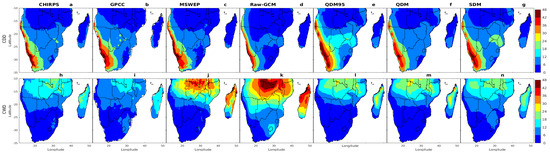
Figure 2.
Climatological (1982–2014) spatial distribution of December-January-February (DJF) CDD (top row) and CWD (bottom row): (a,h) CHIRPS, (b,i) GPCC, (c,j) MSWEP, (d,k) multi-model ensemble (MME) of native simulations, (e,l) MME of QDM95, (f,m) MME of QDM, and (g,n) MME of SDM.
The native GCM multi-model ensemble (MME) significantly underestimated the observed CDD values across much of Southern Africa (Figure 2d) relative to the observational datasets (Figure 2a–c). However, bias correction techniques have improved this underestimation, particularly in western and southern South Africa, the Lesotho Highlands, Botswana, central Mozambique, and southern Madagascar (Figure 2e). While the three bias correction techniques (Figure 2e–g) slightly overestimated the CDD, their values aligned more closely with the observational datasets than the native MME. This overall underestimation of the native CDD was similar across the African regions, as reported in prior studies [44,62,63]. Additionally, Figure 2k shows a substantial CWD frequency pattern, with values exceeding 24 days over northern Southern Africa and Madagascar and moderate values (12–18 days) in the Lesotho-Eswatini region and central Southern Africa. These high CWD values (>30 days) were notably reduced after applying bias correction techniques, especially in northern Southern Africa and Madagascar (Figure 2i–n), reflecting the overall effectiveness of these techniques. Furthermore, the native models generally showed excessive CWD, leading to significant overestimations relative to CHIRPS, GPCC, and MSWEP. This well-documented drizzling bias is prevalent in CMIP6 models [6,64]. Our findings indicate that bias correction techniques improved this bias, resulting in more accurate representations of both the CDD and CWD. The results underscore the importance of bias correction techniques in enhancing the simulation of CDD and CWD extremes in Southern Africa, contributing to more reliable extreme climate impact assessments.
Overall, bias correction techniques significantly improved the alignment of the CDD MME results with CHIRPS, MSWEP, and GPCC, particularly by more accurately representing consecutive wet and dry day spells than the native models. The bias-corrected outputs also showed substantially reduced CWD values, bringing them closer to the CHIRPS and GPCC observations. However, in the northern areas of Southern Africa, the native MME aligned more closely with the MSWEP dataset. These regional and dataset-specific variations emphasize the importance of considering such factors when evaluating the effectiveness of bias correction techniques. Additionally, we observed considerable differences among the three observational datasets in their ability to capture the spatial distribution of the CDD and CWD extreme precipitation indices. Earlier research [3,28,65,66] highlighted similar inconsistencies, underscoring the importance of carefully selecting reference datasets when making comparisons.
3.1.2. Total Number of Rainy Days (RR1) and Heavy (R10mm) and Extremely Heavy Precipitation Days (R20mm)
Figure 3a–g illustrates the geographical distributions of RR1 between the observations and both bias-corrected and native CMIP6 MME simulations. Although the spatial patterns of RR1 exhibited similarities across all datasets, significant discrepancies were evident in the magnitude of RR1, particularly in regions characterized by the highest number of rainy days. For instance, MSWEP exhibited higher RR1 values (∼44 days) than GPCC (∼33 days) and CHIRPS (∼22 days) in the Lesotho-Eswatini region and coastal Angola. Previous studies (e.g., [65]) also reported discrepancies among the observational datasets, particularly in this region.
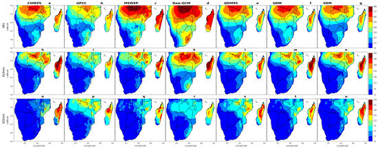
Figure 3.
Climatological (1982–2014) spatial distribution of December-January-February (DJF) RR1 (top row), R10mm (middle row), and R20mm (bottom row): (a,h,o) CHIRPS, (b,i,p) GPCC, (c,j,q) MSWEP, (d,k,r) multi-model ensemble (MME) of native simulations, (e,l,s) MME of QDM95, (f,m,t) MME of QDM, and (g,n,u) MME of SDM.
When comparing the multi-model ensemble (MME) means with the observations, significant differences were noted between the native GCM results (Figure 3d) and the bias-corrected results (Figure 3e–g) in terms of RR1 magnitude and spatial distribution. The native GCM simulations (Figure 3d) showed substantial deviations from the observed datasets (Figure 3a–c), particularly in the Lesotho Highlands, eastern Angola, the northern and eastern parts of Southern Africa, and Madagascar, where regions with more than 66 days of RR1 exhibited marked differences. However, after applying bias correction techniques (QDM95, QDM, and SDM), the native GCM results were adjusted to align more closely with the observations by reducing systematic biases. These corrections significantly improved the accuracy of the CMIP6 models, leading to a more realistic representation of observed RR1 spatial patterns. Notable improvements were evident in areas such as Lesotho, Eswatini, coastal Angola, northern and central Southern Africa, and Madagascar, where the spatial distribution and magnitude of RR1 better matched the observations.
Furthermore, the spatial patterns of heavy precipitation days (R10mm) and extremely heavy precipitation days (R20mm) are shown in Figure 3h–n and Figure 3o–u, respectively. The highest number of days with precipitation exceeding 10 mm and 20 mm occurred along the east coast of Angola, Zambia, Malawi, Mozambique, and northern Zimbabwe, as well as in parts of northern and central Madagascar (Figure 3h–j,o–q). Both the native (Figure 3r–u) and bias-corrected (Figure 3k–n) CMIP6 models captured the general spatial patterns of heavy (R10mm) and extremely heavy (R20mm) precipitation days. However, notable discrepancies remained between the model simulations and observational datasets. Specifically, MSWEP tended to underestimate precipitation maxima associated with orographic features relative to CHIRPS and GPCC. Additionally, the native MME overestimated R10mm (R20mm) in northern Southern Africa and the northern and central highlands of Madagascar, with values exceeding 42 (9) days compared with approximately 36 (8) days in the gridded observations. Conversely, some of the bias-corrected models underestimated R10mm (R20mm) in these regions, with values below 30 (6) days compared with approximately 36 (8) days in the gridded observations. The overestimation and underestimation of RR1 and R10mm (R20mm) precipitation days in these regions may be attributed to the well-known inadequacies of the MME of CMIP6 models in accurately representing complex orographic processes. This issue persisted across all native MMEs, and similar biases in simulating extreme wet and dry precipitation over topographically complex regions have been reported in previous studies [27,44].
3.1.3. Maximum One-Day Precipitation (RX1day), Simple Daily Precipitation Intensity (SDII), and Extremely Wet Days (R95p)
Figure 4a–n illustrates the highest one-day maximum precipitation (RX1day) and the simple daily intensity index (SDII) based on the multi-model ensemble mean over Southern Africa. These two indices exhibited similar spatial distributions but differed in magnitude. Both were generally characterized by high values over northern and eastern Southern Africa and Madagascar, with lower values over the drier western parts of the southern Africa regions.
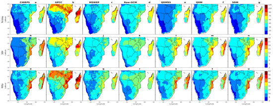
Figure 4.
The same as Figure 3, but for Rx1day (top row), SDII (middle row), and R95p (bottom row).
Figure 4a–c shows the spatial distribution of RX1day precipitation as observed in CHIRPS, GPCC, and MSWEP, respectively. Notable similarities can be observed, particularly in the areas with the lowest RX1day values (less than 30 mm) across Namibia, western South Africa, and western Botswana. However, the datasets showed differences in the total recorded amounts. GPCC (Figure 4b) showed higher RX1day values exceeding 75 mm over Zambia, Malawi, northern and central Mozambique, northeastern Angola, and northern and central Madagascar. In contrast, MSWEP (Figure 4c) and CHIRPS (Figure 4a) exhibited lower RX1day values, with amounts generally under 60 mm in the same regions. Moderate RX1day values (30–75 mm) were generally observed across Angola and northeastern Southern Africa, with maxima exceeding 90 mm concentrated in northern and central Mozambique and eastern Madagascar (Figure 4b). This spatial pattern reflects the influence of moisture-laden air masses originating from the Indian Ocean [54]. Furthermore, the ITCZ plays a crucial role in shaping precipitation patterns across eastern and northern Southern Africa [50,51,67]. During the austral summer, the southward shift of the ITCZ contributes to increased rainfall in these regions.
The native GCM (Figure 4d) overestimated the RX1day values in most of Southern Africa, particularly in the southern and eastern regions and Madagascar. This is evident when comparing the GCM’s spatial extent and intensity to observational datasets (Figure 4a–c), which often showed fewer areas with low RX1day values. After applying bias correction techniques, we significantly reduced these overestimations in many regions, such as northern and eastern Southern Africa, coastal Angola, the Lesotho Highlands, Eswatini, northern Mozambique, and Madagascar (Figure 4e–g).
The spatial distribution of SDII, shown in Figure 4h–j, revealed higher values in northern and eastern Southern Africa and Madagascar, with lower values in the drier western regions. Notably, GPCC (Figure 4i) exhibited higher SDII values than CHIRPS (Figure 4h) and MSWEP (Figure 4j), particularly in regions with frequent heavy precipitation, including coastal Angola, Zambia, Zimbabwe, northern and central Mozambique, and Madagascar. This highlights the variability in precipitation intensity and frequency across the region.
The native GCM (Figure 4k) underestimated the SDII values relative to GPCC (Figure 4i), particularly in the eastern and southern regions, where the native GCM simulated low precipitation intensity. This underestimation was notably improved after bias correction (Figure 4l–n), especially in northern and eastern Southern Africa, coastal Angola, and Madagascar. However, despite these improvements, some underestimation persisted in these regions relative to GPCC.
Furthermore, observational data from CHIRPS, GPCC, and MSWEP (Figure 4o–q), as well as from the native model (Figure 4r) and the three bias-corrected techniques (Figure 4s–u), revealed distinct spatial patterns in R95p precipitation. CHIRPS (Figure 4o) showed high R95p precipitation values along the eastern coastlines and Madagascar, peaking at 60 mm. In contrast, dry regions such as the Kalahari Desert, the adjoining areas of eastern Namibia and western Botswana, and parts of western South Africa experienced significantly lower R95p precipitation levels. GPCC (Figure 4p) exhibited a similar pattern, with slightly higher R95p values observed in the central regions of Southern Africa relative to CHIRPS. MSWEP (Figure 4q) generally showed lower R95p values, but the maxima were still concentrated along the eastern coastlines and Madagascar. These differences in magnitude between the three observations resulted from variations in methodology and horizontal resolution used to calibrate the precipitation intensities. Similar discrepancies have been reported in previous studies when comparing observational datasets, where differences in data sources, interpolation methods, and spatial resolution influenced the recorded precipitation intensities [16]. While our study used different datasets, our findings align with the previous study that highlighted how observational uncertainties contribute to variations in extreme precipitation indices such as R95p.
Significant differences were observed when comparing the multi-model ensemble (MME) means with the observational data, particularly between the results from native global climate models (GCMs) and those after bias correction in terms of the magnitude and spatial distribution of R95p. The native GCM results (Figure 4r) displayed considerable discrepancies with the observed datasets (Figure 4o,q), especially in regions such as the Lesotho Highlands, eastern Angola, and the northern and eastern parts of Southern Africa, including Madagascar. In these areas, discrepancies were noted where R95p values ranged from 24 to 32 mm. However, after employing bias correction techniques—namely QDM95, QDM, and SDM—the native GCM results were adjusted to correspond more closely with the observations, effectively reducing systematic biases. These corrections significantly enhanced the accuracy of the MME from the CMIP6 models, resulting in a more realistic representation of the observed spatial patterns of R95p. Notable improvements were particularly visible in regions such as Lesotho, Eswatini, coastal Angola, northern and central Southern Africa, and Madagascar, where the spatial distribution and magnitude of R95p better aligned with the CHIRPS (Figure 4o) and MSWEP (Figure 4q) datasets.
3.2. Performance of Bias-Corrected and Native MME of CMIP6 GCMs in Simulating Extreme Precipitation Observed by CHIRPS, GPCC, and MSWEP
3.2.1. Geographical Distribution of Biases
Figure 5, Figure 6, Figure 7 and Figure 8 present the spatial distribution of climatological biases for CDD, CWD, RR1, and Rx1day from native GCM ensemble and bias-corrected ensembles (QDM95, QDM, and SDM) relative to the observational datasets (CHIRPS, GPCC, and MSWEP). The native GCM MME (Figure 5a,e,i) exhibited significant underestimations of the CDD across most of Southern Africa, with biases ranging from −5 to −25 days, while overestimations were observed in coastal Angola (relative to CHIRPS and GPCC) and northern Mozambique and Madagascar (relative to MSWEP), with deviations of up to 5 days. These patterns were largely consistent across all three datasets, differing slightly in magnitude. After implementing bias correction techniques, substantial reductions in CDD biases were observed across the study region. For instance, the bias-corrected MME for CHIRPS (Figure 5b–d) reduced biases to a range from approximately −5 to +5 days, while corrections for GPCC (Figure 5f–h) and MSWEP (Figure 5j–l) reduced biases to a range from −10 to +10 days. Overall, the bias correction techniques significantly reduced the large deviations observed in the native GCM MME (Figure 5a,e,i), demonstrating improved alignment with observational datasets across most Southern Africa. Similarly, the native GCM MME significantly overestimated the CWD (Figure 6a,e,i) and RR1 (Figure 7a,e,i) across Southern Africa relative to CHIRPS, GPCC, and MSWEP. Specifically, relative to CHIRPS and GPCC, it overestimated the CWD by amounts exceeding 20 days in regions such as the northern parts of Southern Africa, the Lesotho Highlands, and Madagascar. In contrast, overestimations were observed throughout much of Southern Africa, with biases ranging from 0 to +15 days relative to MSWEP.
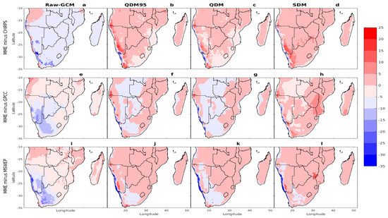
Figure 5.
The climatological biases of the multi-model ensemble (MME) in simulating CDD (days) relative to CHIRPS (top row), GPCC (middle row), and MSWEP (bottom row): (a,e,i) Raw-GCM (native), (b,f,j) QDM95, (c,g,k) QDM, and (d,h,l) SDM.
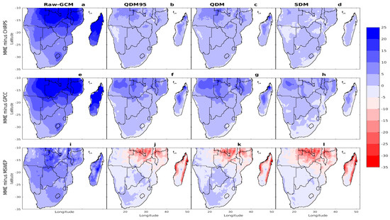
Figure 6.
Same as Figure 5 but for CWD (days).
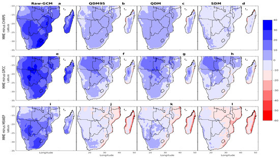
Figure 7.
Same as Figure 5 but for RR1 (days).
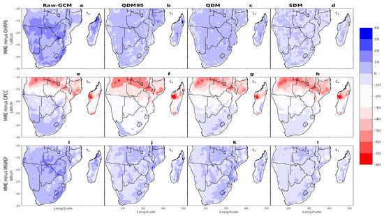
Figure 8.
Same as Figure 5 but for Rx1day (mm).
Following the implementation of bias correction techniques, biases were notably reduced, particularly in northern Southern Africa, the Lesotho Highlands, and Madagascar. Among these techniques, SDM (Figure 6d,h,i) demonstrated the most substantial improvement, followed by QDM95 and QDM. Relative to CHIRPS and GPCC, all bias-corrected techniques reduced positive biases in these regions from up to +25 days to a range from 0 to +10 days. Similarly, negative biases in the southern regions were reduced, shrinking to range between −5 and 0 days. However, compared with MSWEP, all three bias-corrected techniques had a tendency for underestimation. This was expected, since MSWEP is a blended precipitation product that combines satellite and gauge observations, as well as a reanalysis model. Therefore, in areas where observation was lacking, the reanalysis model caused the prediction to suffer from similar model bias.
The MME of both the bias-corrected and native models revealed significant spatial heterogeneity in R10mm (figure not shown here). The MME of the native models underestimated R10mm (ranging from 0 to −10 days) over coastal regions such as Angola, Mozambique, and Madagascar relative to CHIRPS. Conversely, it overestimated R10mm (>+5 days) in central and northern Southern Africa, the Lesotho Highlands, and western and central Madagascar relative to GPCC and MSWEP. This result aligns with the findings of Faye and Akinsanola [47] in West Africa and Rabezanahary et al. [44] in Madagascar, both of whom suggested that CMIP6 models tend to overestimate R10mm in mountain regions (the Lesotho Highlands and the central highlands of Madagascar).
After applying bias correction (QDM95, QDM, and SDM), both overestimation and underestimation biases were reduced across most regions, with biases falling within the range from −5 to +5 days. This finding is consistent with Sian et al. [27], who reported a significant reduction in R10MM biases in native CMIP6 models from an underestimation of up to −45 days to less than 2 days when using the QDM bias correction technique. Therefore, the robustness of the bias-corrected results is evident, with most spatial distributions showing significant improvement.
The MMEs of both bias-corrected and native models showed significant spatial variation in R20mm over Southern Africa, with notable biases relative to CHIRPS, GPCC, and MSWEP (figure not shown here). The native models exhibited underestimations from −10 to 0 days in northern Zambia, Mozambique, southern South Africa, and Madagascar relative to CHIRPS, while bias correction, particularly SDM, reduced these biases to within a range from −2 to +4 days. Relative to GPCC, the native models showed an underestimation of R20mm precipitation over coastal Angola, Zambia, northern Zimbabwe, Mozambique, and Madagascar, with bias values ranging from −8 to −2 days. Conversely, they overestimated R20mm precipitation over Namibia, Botswana, South Africa, the Lesotho Highlands, southern Mozambique, and southern Madagascar, with biases ranging from 0 to +4 days. After applying bias correction techniques, these overestimations and underestimations improved significantly, with the most substantial improvements observed using the QDM95 bias correction technique. Similarly, relative to MSWEP, the native models overestimated R20mm across most of Southern Africa, except in Mozambique and Madagascar. After applying bias correction, QDM effectively reduced these overestimations within a range from −2 to +2 days. Overall, the performance of bias correction techniques depends on the observational dataset. SDM performed best with CHIRPS, QDM95 performed best with GPCC, and QDM performed best with MSWEP, with each significantly improving the R20mm precipitation estimates. This underscores the importance of choosing suitable bias correction techniques and reference datasets.
Overall, the results from the native CMIP6 models in this study are consistent with previous research conducted across Africa. For instance, Ayugi et al. [63] found that CMIP6 GCMs tend to underestimate CDD and R20mm in East Africa, a pattern also observed in other parts of the continent. Similarly, Chen et al. [68] and Rabezanahary et al. [44] suggested that this underestimation may be partly due to the model resolution, which affects how precipitation extremes are simulated. While these studies highlighted persistent biases in CMIP6 models, the present research advances previous work by applying bias correction techniques (QDM95, QDM, and SDM) to improve the simulation of extreme precipitation indices. The results demonstrate that bias correction significantly reduced errors in CDD, CWD, RR1, R10mm, and R20mm, enhancing the reliability of climate projections for Southern Africa. The main contribution of this lies in demonstrating how bias correction can effectively minimize biases, offering a more accurate representation of extreme precipitation patterns in the region, and the variation in the improvement or representativeness of the extremes as a function of the bias correction techniques and reference data used in the bias correction.
3.2.2. Region-Wide Aggregated Performance of CMIP6 Models
Heat maps are important tools for assessing and summarizing the performance of individual models in representing extreme precipitation characteristics relative to the reference datasets [43,44,65]. Figure 9 and Figure 10 show heat maps for eight extreme precipitation indices, highlighting the RMSE and MB of both native and bias-corrected models, along with their multi-model ensembles (MMEs), averaged across the entire study. These evaluations used CHIRPS, GPCC, and MSWEP as reference datasets. The MB and RMSE values exhibited variation as a function of the reference dataset, the extreme precipitation index, the models assessed, and the bias correction techniques applied.
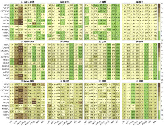
Figure 9.
Heat maps of the mean bias (MB) of each extreme precipitation induced for 11 CMIP6 models and their multi-model ensembles (MMEs) of both native and bias-corrected datasets over Southern Africa, using CHIRPS (top row), GPCC (middle row), and MSWEP (bottom row) as reference datasets.
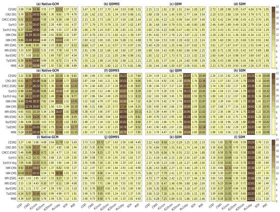
Figure 10.
The same as Figure 9 but for the root mean square error (RMSE).
Figure 9a illustrates that most native CMIP6 models overestimated indices such as CWD, RR1, R10mm, R20mm, and Rx1day, resulting in positive mean biases (MB > 0). For R20mm, only INM-CM4, MPI-ESM1, and TaiESM1 exhibited negative biases of −0.19, −0.69, and −0.14, respectively. Conversely, all models and their MMEs underestimated CDD and SDII, except for MPI-ESM in the case of CDD and MRI-ESM2 in the case of SDII, which displayed positive biases. R95p showed a mix of over- and underestimations. For example, RR1 ranged from a significant overestimation of 7.8 days (MPI-ESM1) to 28.5 days (INM-CM5), while CWD ranged from 4.15 days (NorESM2) to 20.80 days (INM-CM4). Rx1day ranged from an underestimation of −3.38 mm (MPI-ESM1) to an overestimation of 18.16 mm (INM-CM5). These inconsistencies underscore the difficulty of native GCMs in accurately simulating RR1, CWD, Rx1day, and R95p (Figure 9a). After bias correction, the models generally underestimated most indices, particularly with the SDM technique. Nonetheless, significant reductions in biases were achieved for all extreme indices when using QDM95, QDM, and SDM, as shown in Figure 9b–d. For instance, the RR1 bias was reduced to a range from 0.33 days (TaiESM1) to 2.51 days (INM-CM4) for QDM95 (Figure 9b), from 0.22 days (Earth3) to −2.27 days (INM-CM5) for QDM (Figure 9c), and from −1.25 days (MRI-ESM2) to −2.97 days (INM-CM4) for SDM (Figure 9d).
Relative to GPCC, the native models exhibited large negative biases for CDD, RX1day, SDII, and R95p, while showing positive biases for CWD, RR1, and R10mm and mixed biases for R20mm (Figure 9e). After bias correction, CDD, CWD, R10mm, and RR1 showed notable improvement across all techniques (QDM, QDM95, and SDM). However, RX1day and R95p showed limited improvement, highlighting the challenges in correcting biases associated with extreme precipitation events (Figure 9f–h). For SDII, QDM95 demonstrated improvement, whereas QDM and SDM did not. Mixed biases persisted for R20mm after correction. These findings suggest that bias correction techniques can effectively address certain biases, particularly for indices like CDD and CWD, while showing varying performance for indices related to extremes and intensity, with QDM95 showing some potential for SDII. The limited improvement observed for RX1day and R95p might point to a fundamental constraint in quantile distribution methods: the assumption of stationarity. These methods presume that the statistical link between observed and modeled precipitation stays consistent over time. However, extreme precipitation events are frequently impacted by non-stationary factors, such as global warming or changes in land use, which can alter the frequency, intensity, or distribution of extremes, even within the historical period. While correcting spatial precipitation patterns is vital for accurate regional representation, it might not fully account for these evolving influences. As reported previously (e.g., [69,70,71,72,73,74]), non-stationary quantile mapping (NS-QM) offers a way to address this challange by allowing the statistical characteristics of extreme precipitation to change over time or with relevant influencing factors.
Furthermore, the native GCM models generally overestimated the precipitation extremes relative to MSWEP. Most indices, particularly CWD, RR1, R10mm, R20mm, Rx1day, and SDII, exhibited a clear positive bias. For example, INM-CM5 showed the highest positive bias for CWD (14.40 days), RR1 (20.09 days), and RX1day (16.11 mm). While some indices, such as CDD, showed slight underestimations, these were less consistent across the models. Moreover, R95p demonstrated mixed biases; many models slightly overestimated it, while some models (e.g., CMCC-CM2-SR4, CMCC-ESM2, INM-CM4, MPI-ESM1, and TaiESM1) underestimated it. Conversely, CMESM2, Earth3, Earth3-Veg, INM-CM5, MRI-ESM2, NorESM2, and MME tended to overestimate R95p, with biases greater than zero (Figure 9i). QDM95 moderately reduced the positive biases observed in native GCM for most indices. For example, it significantly minimized the biases in Rx1day, with many models showing slightly negative values. Similarly, substantial improvements were observed in CWD, RR1, R10mm, R20mm, SDII, and R95p. However, QDM95 struggled to fully address both dry and wet biases in the precipitation extremes, except for RX1day relative to MSWEP (Figure 9j). The QDM technique consistently reduced the mean bias for most extreme precipitation values across evaluated models. This improvement indicates that QDM effectively minimized both the lower and higher values of the precipitation distribution, aligning model results more closely with the observed extremes relative to MSWEP (Figure 9k). In contrast, the SDM technique showed mixed results. While it reduced the mean bias for extreme precipitation in some models, it retained the mean bias in others, highlighting its sensitivity to individual model characteristics and their specific extreme precipitation distributions (Figure 9l).
Most of the CMIP6 models and their MMEs exhibited substantial discrepancies relative to CHIRPS, GPCC, and MSWEP, as evidenced by high RMSE values ranging from 0 to 22 days (Figure 10a,e,i). However, after applying three bias correction techniques, the RMSE values were significantly reduced to less than 8 days relative to CHIRPS. While indices like RX1day and R95p still showed relatively higher RMSEs, most other indices exhibited significantly reduced RMSE values between 0 and 8 days relative to GPCC and MSWEP. The improvement was particularly pronounced for CHIRPS, where all three bias correction techniques demonstrated significant reductions in RMSE, especially for extreme indices such as CWD, RR1, and RX1day. For instance, QDM95 reduced the RMSE for Rx1day from 18.61 mm (native GCM) to 5.08 mm, while QDM and SDM lowered it to 4.02 mm and 6.34 mm, respectively. Similarly, all three techniques performed effectively for indices such as CWD and RR1, indicating their ability to accurately capture extreme precipitation patterns. However, it is important to note that CHIRPS does not have independent data, since they were used in the bias correction.
Figure 11 and Figure 12 illustrate bar plots of the regional-averaged pattern correlation (PCC) and Taylor skill scores (TSSs) for the native and corrected CMIP6 models, including their multi-model ensemble (MME), across all extreme precipitation indices. Comparisons are presented for three observational datasets: CHIRPS (first column), GPCC (second column), and MSWEP (third column). The PCC and TSS values varied depending on the reference data, index, and each bias-corrected technique.
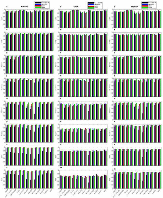
Figure 11.
Pattern correlation coefficient (PCC) for (a–c) consecutive dry days (CDD), (d–f) consecutive wet days (CWD), (g–i) total rain days (RR1), (j–l) heavy precipitation days (R10mm), (m–o) extremely heavy precipitation days (R20mm), (p–r) maximum one-day precipitation (RX1day), (s–u) simple daily intensity index (SDII), and (v–x) extremely wet days (R95p) relative to CHIRPS (first column), GPCC (second column), and MSWEP (third column).
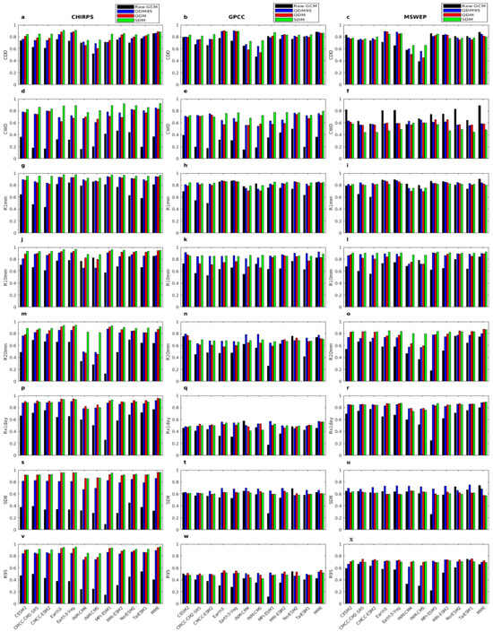
Figure 12.
The same as Figure 11 but for Taylor skill scores (TSSs).
Relative to CHIRPS, the indices CDD (excluding INM-CM4, INM-CM5, and MPI-ESM1), CWD, RR1, R10mm, R20mm, Rx1day, SDII, and R95p demonstrated significant improvement in the performance of CMIP6 models and their MME in reproducing extreme precipitation spatial patterns over Southern Africa (Figure 11, first column). Notably, for most extreme indices, the SDM bias correction technique substantially enhanced the ability of CMIP6 models and their MME to replicate these extreme precipitation spatial patterns relative to CHIRPS. Pattern correlation increased from 0.31 (R20mm)–0.94 (CWD) in the native models to 0.81 (CDD)–0.98 (SDII) after applying the SDM bias correction technique (Figure 11, first column, green bar). Similar improvements were observed with the QDM and QDM95 techniques, with correlation increasing to 0.81 (CDD) and 0.98 (SDII) (Figure 11a,s, blue and red bars) and 0.71 (R20mm) and 0.97 (RR1) (Figure 11g,m, blue and red bars), respectively. The improvements in CWD, SDII, and R95p precipitation are evident from the TSS, which increased significantly after bias correction. For QDM95, the TSS values ranged from 0.61 to 0.89, while for QDM, they ranged from 0.62 to 0.95, and for SDM, the range was from 0.71 to 0.96, compared with the 0.09–0.6 range observed in the native results (Figure 11d,s,v, black bar). Similarly, substantial enhancements were observed in CDD, RR1, R10mm, R20mm, and RX1day, with TSS values improving to 0.49–0.95 for QDM95, 0.46–0.96 for QDM, and 0.81–0.97 for SDM, compared with the native CMIP6 models, which had TSS values of 0.12–0.86 (Figure 12, first column).
Similarly, relative to GPCC, bias correction techniques significantly enhanced both the PCC and TSS of extreme precipitation indices, demonstrating their effectiveness in improving model performance (Figure 11 and Figure 12, second column). SDM produced the most notable improvements, especially for R20mm, where the PCC increased from 0.47 to 0.97, highlighting its proficiency in accurately representing heavy precipitation events. Similarly, the PCC for R95p rose from 0.31 to 0.81, while CWD, CDD, R1mm, and R10mm each achieved a PCC of 0.98 under SDM. These improvements were also evident in the TSS, with CWD’s TSS increasing from 0.19 to 0.79 under SDM, further validating its ability to simulate extreme precipitation. The TSSs for most models reached values above 0.90 (Figure 12, second column). Overall, the best bias correction technique varied across each extreme and each CMIP6 GCM model relative to GPCC (Figure 12, second column).
Additionally, we evaluated the correlation coefficients between different precipitation indices (RR1, CDD, R10mm, CWD, RX1day, SDII, R20mm, and R95) and MSWEP (Figure 11, third column). The three bias correction techniques (QDM95, QDM, and SDM) significantly improved these correlations compared with the native GCM results. The native models exhibited lower correlations, especially for extreme indices such as the SDII (Figure 11u, black bar) and R95 (Figure 11x, black bar), typically being below 0.8. The application of QDM95, QDM, and SDM consistently increased correlation coefficients above 0.9 for the SDII (Figure 11u, blue, red, and green bars) and R95 (Figure 11x, blue, red, and green bars). All models showed significant improvements following bias correction for other extreme indices (R10mm, RX1day, and R20mm). However, for indices like CDD and RR1, the extent of improvement varied across models and bias correction techniques. While some models exhibited substantial enhancements, others showed more limited improvements, highlighting the variable effectiveness of bias correction for different extreme precipitation characteristics. Aside from this, all three bias correction techniques consistently improved the TSS values compared with the native GCM outputs for all precipitation indices relative to MSWEP. The TSS values for extreme indices such as SDII and R95 increased significantly, with all corrected models showing values above 0.8. These improvements were observed across the majority of the indices, demonstrating the effectiveness of bias correction in refining extreme precipitation simulations (Figure 12, third column).
3.2.3. Ranking of CMIP6 Models
Table 2 presents the performance and ranking of native (bias-uncorrected) and bias-corrected CMIP6 GCMs, along with their MME, in simulating all eight extreme precipitation indices across Southern Africa. Our analysis highlights the critical influence of reference data and bias correction techniques on model performance. Models were ranked based on their ability to accurately simulate extreme precipitation, as measured by the CRI values (Table 2). The CRI metric, which reflects this performance, varied substantially. The native GCMs, such as INM-CM4 and MPI-ESM1, exhibited the lowest CRI values (0.01–0.02) and were ranked last, while the bias-corrected models, such as Earth3-Veg, Earth3, and the MME, achieved the highest CRI values (0.96–0.98), ranking first when evaluated relative to the CHIRPS, GPCC, and MSWEP reference datasets.
Table 2.
Comprehensive ranking index (CRI) of native and bias-corrected CMIP6 GCMs for simulating extreme precipitation over Southern Africa relative to CHIRPS, GPCC, and MSWEP for the period of 1982–2014.
Under the SDM bias correction technique, Earth3-Veg achieved the highest CRI of 0.98 relative to CHIRPS, ranking first. It was closely followed by Earth3 and the multi-model ensemble (MME), each with a CRI of 0.95, securing second place. MPI-ESM1 ranked 3rd with a CRI of 0.92, while MRI-ESM2 (0.88), TaiESM1 (0.82), CM2-SR4 (0.80), NorESM2 (0.79), and CMCC-ESM2 (0.76) secured the 5th, 7th, 8th, 9th, and 10th positions, respectively. For the QDM bias correction, the rankings changed relative to CHIRPS. Earth3-Veg (0.84) dropped to 6th, Earth3 (0.79) dropped to 9th, and MME (0.90) ranked 4th, while CM2-SR4 and CMCC-ESM2 retained their 8th and 10th positions, respectively. Similarly, relative to the GPCC observations, under the QDM95 bias correction technique, Earth3 and the MME exhibited the highest CRI of 0.96, sharing the top rank. Earth3-Veg followed closely with a CRI of 0.95, ranking second, while MRI-ESM2 achieved a CRI of 0.83, ranking third. CESM2 (0.78) ranked 5th, with NorESM2 (0.74) and INM-CM5 (0.67) ranked 6th and 10th, respectively. Under the SDM bias correction techniques, Earth3 ranked fourth (CRI 0.79), Earth3-Veg ranked seventh (CRI 0.72), and MRI-ESM2 ranked ninth (CRI 0.70). The MME achieved a CRI of 0.64, ranking 11th. NorESM2 also ranked seventh (CRI 0.72) under the QDM bias correction technique. Furthermore, under the QDM95 bias correction technique, Earth3-Veg (0.97) ranked as the top-performing model relative to the MSWEP reference data, followed closely by Earth3 (0.92) in second place and TaiESM1 (0.86) in third. Meanwhile, MRI-ESM2 (0.85) secured a strong fourth position, whereas the MME (0.83) ranked fifth. Additionally, MPI-ESM1 (0.80) and CMCC-ESM2 (0.76) occupied the seventh and eighth positions, respectively. Conversely, under the QDM bias correction technique, MRI-ESM2 (0.97) secured the first rank relative to MSWEP, while Earth3-Veg (0.81) and Earth3 (0.80) followed in sixth and seventh place, respectively. Moreover, the MME (0.73) was ranked 9th, and NorESM2 (0.71) secured 10th place. These results underscore the differential impact of bias correction techniques across various CMIP6 GCM models when benchmarked against the CHIRPS, GPCC, and MSWEP reference datasets.
These results indicate that bias correction techniques improved the simulation of extreme precipitation indices compared with native models. However, the degree of improvement and the best-performing technique varied across the models and reference datasets. Earth3, Earth3-Veg, and MME consistently outperformed other models across the bias correction techniques, highlighting their reliability in simulating extreme precipitation. Likewise, MPI-ESM1, MRI-ESM2, and CMCC-ESM2 exhibited moderate performance across all three techniques, reinforcing their ability to capture extreme precipitation patterns. This is partly because climate models with higher resolutions generally exhibit improved accuracy in replicating observed extreme precipitation than those with coarser resolutions [65,75]. Nevertheless, Jima et al. [76] found that a higher resolution does not always guarantee better performance. In contrast, the performance of CESM2, CM2-SR5, NorESM2, and TaiESM1 fluctuated, demonstrating that bias correction did not always yield the best results across all metrics and datasets. While QDM95 and SDM offered notable improvements, the most effective technique depended on the specific model and reference dataset. However, some models, such as INM-CM4 and INM-CM5, consistently underperformed both before and after bias correction, highlighting inherent limitations in their ability to simulate extreme precipitation accurately. This finding aligns with previous research [44,77,78], which reported similar performance issues with lower-resolution models, suggesting a fundamental challenge in capturing extreme precipitation.
Our results highlight the influence of reference datasets on bias correction results, as different models responded variably to bias correction techniques. This aligns with previous studies [28,79,80,81], which emphasized the role of observational uncertainties in bias correction performance. Additionally, model rankings and performance assessments shifted depending on the chosen reference dataset, as observed in comparisons between CHIRPS and MSWEP [28]. This underscores the necessity of incorporating multiple observational datasets to enhance the robustness of extreme climate model simulations and reduce uncertainties in extreme precipitation projections. Furthermore, our findings demonstrate that the MME, Earth3, and Earth3-Veg models generally outperformed individual models. However, no single model was consistently ranked the best across all bias correction techniques relative to CHIRPS, GPCC, and MSWEP. This challenge of identifying a clear top-performing model has been reported in studies on Brazil, Madagascar, and sub-Saharan Africa [28,44,82]. While MMEs often outperform individual models due to the averaging of structural and parametric uncertainties [83,84], their relative performance can fluctuate based on (1) the characteristics of the reference dataset, (2) how bias correction modifies inter-model variability, and (3) the nonlinear interactions between model spread and ensemble averaging [85]. Moreover, the observed variation in CRI rankings indicates that bias correction techniques did not uniformly benefit all models. Techniques such as QDM, QDM95, and SDM have differing assumptions about the preservation of quantiles, distributional shape, and trends [86,87,88]. Some techniques, like SDM, may overly constrain interannual variability, while others like QDM95 may better preserve the distribution tails, influencing how well specific models reproduce observed patterns. Finally, the choice of observational reference (CHIRPS, GPCC, or MSWEP) also affects CRI rankings due to inherent differences in their gauge densities, blending techniques, and temporal coverage [35,36,38]. These observational uncertainties further contribute to the observed variability in model performance and ensemble skill across different configurations.
4. Conclusions
Extreme climate events are becoming more frequent and intense, posing considerable hazards to important sectors around the world. Addressing these challenges requires understanding the spatial characteristics of extreme climate events and regional climate responses. Accurate simulation of extreme precipitation is crucial for managing climate-sensitive sectors in Southern Africa, such as water resources, agriculture, and infrastructure. However, global climate models often fail to capture these events accurately, limiting their practical application. Bias correction techniques are crucial in enhancing the accuracy of extreme climate simulations. This research explored the potential of three bias correction techniques, namely quantile distribution mapping (QDM), separate quantile distribution mapping for precipitation equal to or less than the 95th percentile and greater than the 95th percentile (QDM95), and scaled distribution mapping (SDM), to enhance the simulation of extreme precipitation in Southern Africa using 11 CMIP6 models.
The findings demonstrate that there were notable differences in the amount and geographical distribution of extreme precipitation in the MME of native CMIP6 GCM outputs, especially over complex terrains and high-altitude regions. However, bias correction techniques reduced these biases. The MME of native CMIP6 GCM models typically underestimated the CDD and overestimated the CWD. Bias correction largely reduced these errors, though some overestimation of CWD and underestimation of CDD persisted. Similarly, the MME of raw CMIP6 GCM models overestimated RR1, R10mm, and R20mm, particularly in Madagascar and northern Southern Africa. Bias correction significantly reduced the magnitude of overestimation in these precipitation indices, resulting in better agreement with the three observed datasets. After bias correction, extreme precipitation indices, such as RX1day, SDII, and R95p, exhibited improved spatial patterns. However, regional variations persisted, which were largely influenced by topographic characteristics. These variations were evident relative to CHIRPS, GPCC, and MSWEP.
Furthermore, this study demonstrated the impact of bias correction using various performance metrics, including MB, RMSE, PCC, and TSS, for precipitation indices such as R20mm, SDII, CWD, R95p, RR1, Rx1day, R10mm, and CDD. The native CMIP6 models exhibited systematic biases, with large positive biases for CWD, RR1, and R10mm and negative biases for Rx1day, SDII, and R95p, especially relative to GPCC, except for some models. Similarly, the native models showed significant negative biases for CDD, Rx1day, SDII, and R95p and positive biases for CWD, RR1, and R10mm relative to CHIRPS. For MSWEP, most indices were overestimated, with INM-CM5 showing the largest bias. The CMIP6 models and their MMEs exhibited substantial differences relative to observational datasets such as CHIRPS, GPCC, and MSWEP, as indicated by high RMSE values. After applying the three bias correction techniques (QDM, QDM95, and SDM), both the MB and RMSE values were significantly reduced for all extreme indices relative to CHIRPS. Relative to GPCC, the errors for all indices, except Rx1day and R95p, were reduced. The lack of error reduction for Rx1day and R95p might be due to factors related to coarse resolution or the specific characteristics of these indices that GPCC may not fully capture. Additionally, relative to MSWEP, the highest values for the MB and RMSE for CWD and RR1 did not decrease for any of the bias correction techniques. This could be because MSWEP was obtained from the integration of satellite, ground observations, and reanalysis datasets.
Pattern correlation (PCC) for extreme precipitation indices (R20mm, Rx1day, SDII, R10mm, CDD, RR1, R95p, and CWD) showed substantial improvement relative to CHIRPS. SDM yielded the most significant gains, increasing the PCC from 0.31–0.94 in the native models to 0.81–0.98 post-correction. QDM and QDM95 also demonstrated notable improvements, with PCC values generally exceeding 0.8 after bias correction. Similarly, the TSS values improved, particularly for SDM, reaching from 0.71 to 0.96. Relative to GPCC and MSWEP, the PCC exceeded 0.8 for most indices. However, the degree of improvement varied across indices and models. While bias correction generally increased the PCC and TSSs for extreme indices relative to CHIRPS, GPCC, and MSWEP, CWD showed no significant increments in PCC or TSS relative to MSWEP.
The ranking of native and bias-corrected CMIP6 models in simulating all eight extreme precipitation indices was strongly influenced by the choice of bias correction technique and reference dataset. When CHIRPS was used as a reference, Earth3-Veg performed best under the SDM bias correction technique. However, under QDM95, this model ranked first with MSWEP as the reference and second with GPCC. Similarly, when MSWEP was used as a reference, Earth3-Veg and MRI-ESM2 were the top-performing models under QDM95 and QDM, respectively. However, when GPCC was used as the reference dataset, Earth3-Veg ranked second under QDM, while MRI-ESM2 ranked third under QDM95. Overall, bias correction improved the model rankings, with Earth3-Veg, Earth3, MRI-ESM2, and MME consistently performing well, while native models like INM-CM4 and MPI-ESM1 ranked the lowest. The effectiveness of each technique varied by reference dataset, with QDM95 and SDM generally enhancing model reliability. However, some models, such as INM-CM4 and INM-CM5, remained low in rank even after correction, suggesting limitations in capturing extreme precipitation. These findings emphasize the importance of reference datasets in model evaluations and the need for multiple observational datasets. While higher-resolution models tended to perform better, their effectiveness remained context-dependent. Future research should refine bias correction techniques and explore ensemble approaches to improve extreme precipitation simulations.
In general, this study highlights the importance of bias correction in improving the reliability of the CMIP6 models’ extreme precipitation simulations in Southern Africa. This is particularly important for climate scientists and policymakers who rely on bias-corrected models for impact assessments and formulating adaptation strategies to mitigate the impacts of future precipitation changes. This study underscores the importance of selecting suitable bias correction techniques based on relevant observational data and the target extreme events. These findings improve our understanding of how bias correction enhances climate model accuracy in representing extreme precipitation, which is essential for regional impact studies. Future research should explore the performance of these techniques across various regions to refine bias correction techniques for broader climate modeling.
Based on the findings of this study, the following recommendations are proposed:
- Given the variability in model performance relative to different observational datasets (CHIRPS, GPCC, and MSWEP), the use of multiple reference datasets is vital for robust model evaluation and bias correction.
- No single technique (QDM, QDM95, or SDM) outperformed the others across all indices and datasets. The selection of bias correction methods should consider the characteristics of the extremes being studied. For example, QDM95 may be more suitable for high-impact events such as Rx1day, while SDM offers improved spatial pattern fidelity.
- While MMEs reduce individual model errors, their skill varies by metric, reference dataset, and correction technique. High-performing models like Earth3-Veg and MRI-ESM2 sometimes outperform the MME, suggesting that ensemble mean approaches should be used cautiously. Knutti et al. [84] cautioned against overreliance on MMEs and advocated for performance-based selection.
- Persistent biases over high-altitude regions even after correction indicate the need for improved physical representations in GCMs. Enhanced resolutions and improved parameterizations of convective and orographic processes are essential, echoing the findings of Giorgi et al. [89], Déqué et al. [90], and Ban et al. [91].The inability of conventional techniques to fully address biases in some indices suggests the need for hybrid or adaptive approaches. These may include regional tuning or the integration of machine learning methods. Recent studies such as those by Vrac and Friederichs [92] and Gutmann et al. [93] advocate for data-driven and adaptive correction schemes.
Author Contributions
A.A.A., as the primary analyst and drafter, handled the methodology, statistical data analysis, visualization, and initial manuscript creation and refinement. G.M.T., serving as the conceptual lead and supervisor, contributed to the methodology, analysis, visualization, and all stages of manuscript development. L.V.B., in a supervisory and editorial capacity, reviewed and edited the manuscript. All authors have read and agreed to the published version of the manuscript.
Funding
This study received funding from the O.R. Tambo Africa Research Chairs Initiative, supported by the Ministry of Tertiary Education, the Botswana International University of Science and Technology, the Department of Science and Innovation of South Africa (DSI), the National Research Foundation of South Africa (NRF), the Oliver & Adelaide Tambo Foundation (OATF), and the International Development Research Center of Canada (IDRC), with grant number: (UID)136696.
Data Availability Statement
The bias-corrected data are available upon request.
Acknowledgments
The authors gratefully acknowledge that the CMIP6 simulations used in our data analyses are freely available from the Earth System Grid Federation (https://esgf-node.llnl.gov/search/cmip6). We also thank the providers of the GPCC and CHIRPS datasets, which are freely available at https://cds.climate.copernicus.eu/datasets, and the MSWEP dataset, which is freely accessible at https://www.gloh2o.org/mswep/. All URLs were last accessed on 29 April 2025.
Conflicts of Interest
The authors declare that they have no competing interests.
References
- Easterling, D.R.; Evans, J.; Groisman, P.Y.; Karl, T.R.; Kunkel, K.E.; Ambenje, P. Observed variability and trends in extreme climate events: A brief review. Bull. Am. Meteorol. Soc. 2000, 81, 417–426. [Google Scholar] [CrossRef]
- Lu, L.-C.; Chiu, S.-Y.; Chiu, Y.-H.; Chang, T.-H. Sustainability efficiency of climate change and global disasters based on greenhouse gas emissions from the parallel production sectors—A modified dynamic parallel three-stage network dea model. J. Environ. Manag. 2022, 317, 115401. [Google Scholar] [CrossRef] [PubMed]
- Gibba, P.; Sylla, M.B.; Okogbue, E.C.; Gaye, A.T.; Nikiema, M.; Kebe, I. State-of-the-art climate modeling of extreme precipitation over Africa: Analysis of CORDEX added-value over CMIP5. Theor. Appl. Climatol. 2019, 137, 1041–1057. [Google Scholar] [CrossRef]
- Lee, H.; Calvin, K.; Dasgupta, D.; Krinner, G.; Mukherji, A.; Thorne, P.; Park, Y. IPCC, 2023: Climate Change 2023: Synthesis Report, Summary for Policymakers; Contribution of Working Groups I, II and III to the Sixth Assessment Report of the Intergovernmental Panel on Climate Change; Core Writing Team, Lee, H., Romero, J., Eds.; IPCC: Geneva, Switzerland, 2023. [Google Scholar]
- Hove, L.; Kambanje, C. Lessons from the el nino–induced 2015/16 drought in the southern africa region. In Current Directions in Water Scarcity Research; Elsevier: Amsterdam, The Netherlands, 2019; Volume 2, pp. 33–54. [Google Scholar]
- Flato, G.; Marotzke, J.; Abiodun, B.; Braconnot, P.; Chou, S.C.; Collins, W.; Cox, P.; Driouech, F.; Emori, S.; Eyring, V.; et al. Evaluation of climate models. In Climate Change 2013: The Physical Science Basis; Contribution of Working Group I to the Fifth Assessment Report of the Intergovernmental Panel on Climate Change; Cambridge University Press: Cambridge, UK, 2014; pp. 741–866. [Google Scholar]
- Chikowore, G.; Nhavira, J.; Munhande, C.; Mashingaidze, T.; Sibanda, M. Natural disasters and development opportunities: Cyclone idai, challenges, integration and development alternatives in Zimbabwe and sub-Saharan Africa in the new millennium. Fountain J. Interdiscip. Stud. 2019, 3, 1–14. [Google Scholar]
- Macamo, C. After idai: Insights from mozambique for climate resilient coastal infrastructure. Policy Insights Afr. Perspect. Glob. Insights 2021, 110, 1–22. [Google Scholar]
- Konapala, G.; Mishra, A.K.; Wada, Y.; Mann, M.E. Climate change will affect global water availability through compounding changes in seasonal precipitation and evaporation. Nat. Commun. 2020, 11, 3044. [Google Scholar] [CrossRef]
- Wehner, M.; Lee, J.; Risser, M.; Ullrich, P.; Gleckler, P.; Collins, W.D. Evaluation of extreme sub-daily precipitation in high-resolution global climate model simulations. Philos. Trans. R. Soc. A 2021, 379, 20190545. [Google Scholar] [CrossRef]
- Erlich, C.; McDonald, A.; Schuddeboom, A.; Vishwanathan, G.; Renwick, J.; Rana, S. Positive correlation between wet-day frequency and intensity linked to universal precipitation drivers. Nat. Geosci. 2023, 16, 410–415. [Google Scholar]
- Fowler, H.J.; Blenkinsop, S.; Tebaldi, C. Linking climate change modelling to impacts studies: Recent advances in downscaling techniques for hydrological modelling. Int. J. Climatol. J. R. Meteorol. Soc. 2007, 27, 1547–1578. [Google Scholar] [CrossRef]
- Hossein, P.; Tabari, H.; Willems, P. Climate change impact on short-duration extreme precipitation and intensity–duration–frequency curves over europe. J. Hydrol. 2020, 590, 125249. [Google Scholar]
- Sun, C.; Liang, X.-Z. Improving us extreme precipitation simulation: Sensitivity to physics parameterizations. Clim. Dyn. 2020, 54, 4891–4918. [Google Scholar] [CrossRef]
- Li, F.; Collins, W.D.; Wehner, M.F.; Williamson, D.L.; Olson, J.G. Response of precipitation extremes to idealized global warming in an aqua-planet climate model: Towards a robust projection across different horizontal resolutions. Tellus A Dyn. Meteorol. Oceanogr. 2011, 63, 876–883. [Google Scholar] [CrossRef]
- Crétat, J.; Vizy, E.K.; Cook, K.H. How well are daily intense rainfall events captured by current climate models over africa? Clim. Dyn. 2014, 42, 2691–2711. [Google Scholar] [CrossRef]
- Huang, B.; Liu, Z.; Liu, S.; Duan, Q. Investigating the performance of cmip6 seasonal precipitation predictions and a grid based model heterogeneity oriented deep learning bias correction framework. J. Geophys. Atmos. 2023, 128, e2023JD039046. [Google Scholar] [CrossRef]
- Mishra, A.K.; Dubey, A.K.; Dinesh, A.S. Diagnosing whether the increasing horizontal resolution of regional climate model inevitably capable of adding value: Investigation for indian summer monsoon. Clim. Dyn. 2023, 60, 1925–1945. [Google Scholar] [CrossRef]
- Casanueva, A.; Herrera, S.; Iturbide, M.; Lange, S.; Jury, M.; Dosio, A.; Maraun, D.; Gutiérrez, J.M. Testing bias adjustment methods for regional climate change applications under observational uncertainty and resolution mismatch. Atmos. Sci. Lett. 2020, 21, e978. [Google Scholar] [CrossRef]
- Tabari, H.; Paz, S.M.; Buekenhout, D.; Willems, P. Comparison of statistical downscaling methods for climate change impact analysis on precipitation-driven drought. Hydrol. Earth Syst. Sci. 2021, 25, 3493–3517. [Google Scholar] [CrossRef]
- Jaiswal, R.; Mall, R.; Singh, N.; Lakshmi Kumar, T.; Niyogi, D. Evaluation of bias correction methods for regional climate models: Downscaled rainfall analysis over diverse agroclimatic zones of india. Earth Space Sci. 2022, 9, e2021EA001981. [Google Scholar] [CrossRef]
- Gumindoga, W.; Rientjes, T.H.; Haile, A.T.; Makurira, H.; Reggiani, P. Performance of bias-correction schemes for cmorph rainfall estimates in the zambezi river basin. Hydrol. Earth Syst. Sci. 2019, 23, 2915–2938. [Google Scholar] [CrossRef]
- Chen, J.; Brissette, F.P.; Chaumont, D.; Braun, M. Finding appropriate bias correction methods in downscaling precipitation for hydrologic impact studies over north america. Water Resour. Res. 2013, 49, 4187–4205. [Google Scholar] [CrossRef]
- Ayugi, B.; Tan, G.; Ruoyun, N.; Babaousmail, H.; Ojara, M.; Wido, H.; Mumo, L.; Ngoma, N.H.; Nooni, I.K.; Ongoma, V. Quantile mapping bias correction on rossby centre regional climate models for precipitation analysis over Kenya, East Africa. Water 2020, 12, 801. [Google Scholar] [CrossRef]
- Hamadalnel, M.; Zhu, Z.; Gaber, A.; Iyakaremye, V.; Ayugi, B. Possible changes in sudan’s future precipitation under the high and medium emission scenarios based on bias adjusted gcms. Atmos. Res. 2022, 269, 106036. [Google Scholar] [CrossRef]
- Bellprat, O.; Lott, F.C.; Gulizia, C.; Parker, H.R.; Pampuch, L.A.; Pinto, I.; Ciavarella, A.; Stott, P.A. Unusual past dry and wet rainy seasons over southern africa and south america from a climate perspective. Weather Clim. Extrem. 2015, 9, 36–46. [Google Scholar] [CrossRef]
- Sian, K.T.C.L.K.; Hagan, D.F.T.; Ayugi, B.O.; Nooni, I.K.; Ullah, W.; Babaousmail, H.; Ongoma, V. Projections of precipitation extremes based on bias-corrected coupled model intercomparison project phase 6 models ensemble over southern africa. Int. J. Climatol. 2022, 42, 8269–8289. [Google Scholar] [CrossRef]
- Samuel, S.; Mengistu Tsidu, G.; Dosio, A.; Mphale, K. Assessment of historical and future mean and extreme precipitation over sub-saharan africa using nex-gddp-cmip6: Part i—Evaluation of historical simulation. Int. J. Climatol. 2025, 45, e8672. [Google Scholar] [CrossRef]
- Samuel, S.; Dosio, A.; Mphale, K.; Faka, D.N.; Wiston, M. Comparison of multimodel ensembles of global and regional climate models projections for extreme precipitation over four major river basins in southern africa—Assessment of the historical simulations. Clim. Change 2023, 176, 57. [Google Scholar] [CrossRef]
- Muller, A.; Reason, C.; Fauchereau, N. Extreme rainfall in the namib desert during late summer 2006 and influences of regional ocean variability. Int. J. Climatol. J. R. Meteorol. 2008, 28, 1061–1070. [Google Scholar] [CrossRef]
- Rapolaki, R.S.; Reason, C.J. Tropical storm chedza and associated floods over south-eastern africa. Nat. Hazards 2018, 93, 189–217. [Google Scholar] [CrossRef]
- McBride, C.M.; Kruger, A.C.; Dyson, L. Changes in extreme daily rainfall characteristics in south africa: 1921–2020. Weather Clim. 2022, 38, 100517. [Google Scholar]
- Addisuu, A.A.; Mengistu Tsidu, G.; Basupi, L.V. Improving Daily CMIP6 Precipitation in Southern Africa Through Bias Correction—Part 1: Spatiotemporal Characteristics. Climate, 2025; accepted for publication. [Google Scholar]
- NOAA National Geophysical Data Center. 2-Minute Gridded Global Relief Data (ETOPO2) v2; NOAA National Centers for Environmental Information: Asheville, NC, USA, 2006. [Google Scholar]
- Funk, C.; Peterson, P.; Landsfeld, M.; Pedreros, D.; Verdin, J.; Shukla, S.; Husak, G.; Rowland, J.; Harrison, L.; Hoell, A. The climate hazards infrared precipitation with stations—A new environmental record for monitoring extremes. Sci. Data 2015, 2, 1–21. [Google Scholar] [CrossRef]
- Beck, H.E.; Pan, M.; Roy, T.; Weedon, G.P.; Pappenberger, F.; Van Dijk, A.I.J.M.; Huffman, G.J.; Adler, R.F.; Wood, E.F. Daily Evaluation of 26 Precipitation Datasets Using Stage-IV Gauge-Radar Data for the CONUS. Hydrol. Earth Syst. Sci. 2019, 23, 207–224. [Google Scholar] [CrossRef]
- Mekonnen, K.; Velpuri, N.M.; Leh, M.; Akpoti, K.; Owusu, A.; Tinonetsana, P.; Hamouda, T.; Ghansah, B.; Paranamana, T.P.; Munzimi, Y. Accuracy of satellite and reanalysis rainfall estimates over africa: A multi-scale assessment of eight products for continental applications. J. Hydrol. Reg. Stud. 2023, 49, 101514. [Google Scholar] [CrossRef]
- Schneider, U.; Becker, A.; Finger, P.; Meyer-Christoffer, A.; Ziese, M.; Rudolf, B. GPCC’s new land surface precipitation climatology based on quality-controlled in situ data and its role in quantifying the global water cycle. Theor. Appl. Climatol. 2014, 115, 15–40. [Google Scholar] [CrossRef]
- Karl, T.R.; Easterling, D.R. Climate extremes: Selected review and future research directions. Clim. Change 1999, 42, 309–325. [Google Scholar] [CrossRef]
- Sillmann, J.; Kharin, V.; Zhang, X.; Zwiers, F.; Bronaugh, D. Climate extremes indices in the cmip5 multimodel ensemble: Part 1. model evaluation in the present climate. J. Geophys. Res. Atmos. 2013, 118, 1716–1733. [Google Scholar] [CrossRef]
- Chervenkov, H.; Slavov, K. Etccdi climate indices for assessment of the recent climate over southeast europe. In Advances in High Performance Computing: Results of the International Conference on “High Performance Computing” Borovets, Bulgaria, 2019; Springer: Berlin/Heidelberg, Germany, 2021; pp. 398–412. [Google Scholar] [CrossRef]
- Sillmann, J.; Kharin, V.V.; Zwiers, F.W.; Zhang, X.; Bronaugh, D. Climate extremes indices in the cmip5 multimodel ensemble: Part 2. future climate projections. J. Geophys. Atmos. 2013, 118, 2473–2493. [Google Scholar] [CrossRef]
- Akinsanola, A.; Kooperman, G.; Pendergrass, A.; Hannah, W.; Reed, K. Seasonal representation of extreme precipitation indices over the united states in cmip6 present-day simulations. Environ. Res. Lett. 2020, 15, 094003. [Google Scholar] [CrossRef]
- Rabezanahary Tanteliniaina, M.F.; Zhai, J.; Andrianarimanana, M.H. Performance evaluation of cmip6 in simulating extreme precipitation in madagascar. Theor. Appl. Climatol. 2024, 155, 4089–4100. [Google Scholar] [CrossRef]
- Usman, M.T.; Reason, C. Dry spell frequencies and their variability over southern africa. Clim. Res. 2004, 26, 199–211. [Google Scholar] [CrossRef]
- Thoithi, W.; Blamey, R.C.; Reason, C.J. Dry spells, wet days, and their trends across southern africa during the summer rainy season. Geophys. Res. Lett. 2021, 48, e2020GL091041. [Google Scholar] [CrossRef]
- Faye, A.; Akinsanola, A.A. Evaluation of extreme precipitation indices over west africa in cmip6 models. Clim. Dyn. 2022, 58, 925–939. [Google Scholar] [CrossRef]
- Klutse, N.A.B.; Quagraine, K.A.; Nkrumah, F.; Quagraine, K.T.; Berkoh-Oforiwaa, R.; Dzrobi, J.F.; Sylla, M.B. The climatic analysis of summer monsoon extreme precipitation events over west africa in cmip6 simulations. Earth Syst. Environ. 2021, 5, 25–41. [Google Scholar] [CrossRef]
- Chongue, L.A.; Nishii, K. The influence of tropical and subtropical modes of climate variability on precipitation in mozambique. Int. Climatol. 2024, 44, 2993–3005. [Google Scholar] [CrossRef]
- Dunning, C.M.; Black, E.C.; Allan, R.P. The onset and cessation of seasonal rainfall over africa. J. Geophys. Res. Atmos. 2016, 121, 11–405. [Google Scholar] [CrossRef]
- Nicholson, S.E. The itcz and the seasonal cycle over equatorial africa. Bull. Am. Meteorol. Soc. 2018, 99, 337–348. [Google Scholar] [CrossRef]
- Ratna, S.B.; Ratnam, J.; Behera, S.; Rautenbach, C.; Ndarana, T.; Takahashi, K.; Yamagata, T. Performance assessment of three convective parameterization schemes in wrf for downscaling summer rainfall over south africa. Clim. Dyn. 2014, 42, 2931–2953. [Google Scholar] [CrossRef]
- Weber, T.; Cabos, W.; Sein, D.V.; Jacob, D. Benefits of simulating precipitation characteristics over africa with a regionally-coupled atmosphere—Ocean model. Clim. Dyn. 2023, 60, 1079–1102. [Google Scholar] [CrossRef]
- Rouault, M.; Dieppois, B.; Tim, N.; Hünicke, B.; Zorita, E. Southern Africa Climate Over the Recent Decades: Description, Variability and Trends. In Sustainability of Southern African Ecosystems under Global Change: Science for Management and Policy Interventions; Springer: Berlin/Heidelberg, Germany, 2024; pp. 149–168. [Google Scholar] [CrossRef]
- Jones, P.W. First-and Second-Order Conservative Remapping Schemes for Grids in Spherical Coordinates; Mon. Weather. Rev. 1999, 127, 2204–2210. [Google Scholar] [CrossRef]
- Herrera, S.; Gutiérrez, J.M.; Ancell, R.; Pons, M.R.; Frías, M.D.; Fernández, J. Development and Analysis of a 50-Year High-Resolution Daily Gridded Precipitation Dataset over Spain (Spain02). Int. J. Climatol. 2012, 32, 74–85. [Google Scholar] [CrossRef]
- Hofstra, N.; Haylock, M.; New, M.; Jones, P.; Frei, C. Comparison of Six Methods for the Interpolation of Daily European Climate Data. J. Geophys. Res. Atmos. 2008, 113, D21. [Google Scholar] [CrossRef]
- Gordon, N.D.; Shaykewich, J. Guidelines on Performance Assessment of Public Weather Services; World Meteorological Organization: Geneva, Switzerland, 2000. [Google Scholar]
- Tyson, P. Atmospheric circulation changes and palaeoclimates of Southern Africa. S. Afr. J. Sci. 1999, 95, 194–201. [Google Scholar]
- Cook, C.; Reason, C.J.; Hewitson, B.C. Wet and dry spells within particularly wet and dry summers in the South African summer rainfall region. Clim. Res. 2004, 26, 17–31. [Google Scholar] [CrossRef]
- Reason, C.; Hachigonta, S.; Phaladi, R. Interannual variability in rainy season characteristics over the limpopo region of Southern Africa. Int. J. Climatol. J. R. Meteorol. 2005, 25, 1835–1853. [Google Scholar] [CrossRef]
- Ogega, O.M.; Koske, J.; Kung’u, J.B.; Scoccimarro, E.; Endris, H.S.; Mistry, M.N. Heavy precipitation events over east africa in a changing climate: Results from cordex rcms. Clim. Dyn. 2020, 55, 993–1009. [Google Scholar] [CrossRef]
- Ayugi, B.; Zhihong, J.; Zhu, H.; Ngoma, H.; Babaousmail, H.; Rizwan, K.; Dike, V. Comparison of cmip6 and cmip5 models in simulating mean and extreme precipitation over east africa. Int. J. Climatol. 2021, 41, 6474–6496. [Google Scholar] [CrossRef]
- Trenberth, K.E.; Zhang, Y. How often does it really rain? Bull. Am. Meteorol. Soc. 2018, 99, 289–298. [Google Scholar] [CrossRef]
- Samuel, S.; Mengistu Tsidu, G.; Dosio, A.; Mphale, K. Exploring the influence of improved horizontal resolution on extreme precipitation in Southern Africa major river basins: Insights from cmip6 highresmip simulations. Clim. Dyn. 2024, 62, 8099–8120. [Google Scholar] [CrossRef]
- Sylla, M.; Giorgi, F.; Coppola, E.; Mariotti, L. Uncertainties in daily rainfall over africa: Assessment of gridded observation products and evaluation of a regional climate model simulation. Int. J. Climatol. 2013, 33, 1805–1817. [Google Scholar] [CrossRef]
- Pinto, I.; Lennard, C.; Tadross, M.; Hewitson, B.; Dosio, A.; Nikulin, G.; Panitz, H.-J.; Shongwe, M.E. Evaluation and projections of extreme precipitation over southern africa from two cordex models. Clim. Change 2016, 135, 655–668. [Google Scholar] [CrossRef]
- Chen, H.; Sun, J.; Lin, W.; Xu, H. Comparison of cmip6 and cmip5 models in simulating climate extremes. Sci. Bull. 2020, 65, 1415–1418. [Google Scholar] [CrossRef]
- Cannon, A.J.; Sobie, S.R.; Murdock, T.Q. Bias correction of GCM precipitation by quantile mapping: How well do methods preserve changes in quantiles and extremes? J. Clim. 2015, 28, 6938–6959. [Google Scholar] [CrossRef]
- Pierce, D.W.; Cayan, D.R.; Maurer, E.P.; Abatzoglou, J.T.; Hegewisch, K.C. Improved bias correction techniques for hydrological simulations of climate change. J. Hydrometeorol. 2015, 16, 2421–2442. [Google Scholar] [CrossRef]
- Vrac, M.; Noël, T.; Vautard, R. Bias correction of precipitation through Singularity Stochastic Removal: Because occurrences matter. J. Geophys. Res. Atmos. 2016, 121, 5237–5258. [Google Scholar] [CrossRef]
- Vidrio-Sahagún, C.T.; He, J. The decomposition-based nonstationary flood frequency analysis. J. Hydrol. 2022, 612, 128186. [Google Scholar] [CrossRef]
- Vidrio-Sahagún, C.T.; Ruschkowski, J.; He, J.; Pietroniro, A. A practice-oriented framework for stationary and nonstationary flood frequency analysis. Environ. Model. Softw. 2024, 173, 105940. [Google Scholar] [CrossRef]
- Vidrio-Sahagún, C.T.; He, J.; Pietroniro, A. Improved Correction of Extreme Precipitation through Explicit and Continuous Nonstationarity Treatment and the Metastatistical Approach. Water Resour. Res. 2025, 61, e2024WR037721. [Google Scholar] [CrossRef]
- Agel, L.; Barlow, M. How well do cmip6 historical runs match observed northeast us precipitation and extreme precipitation–related circulation. J. Clim. 2020, 33, 9835–9848. [Google Scholar] [CrossRef]
- Jima, W.L.; Bahaga, T.K.; Mengistu Tsidu, G. Fidelity of cmip6 models in simulating june–september rainfall climatology, spatial and trend patterns over complex topography of greater horn of Africa. Pure Appl. Geophys. 2024, 181, 577–609. [Google Scholar] [CrossRef]
- Ge, F.; Zhu, S.; Luo, H.; Zhi, X.; Wang, H. Future changes in precipitation extremes over southeast asia: Insights from cmip6 multi-model ensemble. Environ. Res. Lett. 2021, 16, 024013. [Google Scholar] [CrossRef]
- Srivastava, A.; Grotjahn, R.; Ullrich, P.A. Evaluation of historical cmip6 model simulations of extreme precipitation over contiguous us regions. Weather Clim. Extrem. 2020, 29, 100268. [Google Scholar] [CrossRef]
- Prein, A.F.; Gobiet, A. Impacts of uncertainties in european gridded precipitation observations on regional climate analysis. Int. J. Climatol. 2017, 37, 305–327. [Google Scholar] [CrossRef] [PubMed]
- Gampe, D.; Schmid, J.; Ludwig, R. Impact of reference dataset selection on rcm evaluation, bias correction, and resulting climate change signals of precipitation. J. Hydrometeorol. 2019, 20, 1813–1828. [Google Scholar] [CrossRef]
- Kotlarski, S.; Szabó, P.; Herrera, S.; Räty, O.; Keuler, K.; Soares, P.M.; Cardoso, R.M.; Bosshard, T.; Pagé, C.; Boberg, F.; et al. Observational uncertainty and regional climate model evaluation: A pan-european perspective. Int. J. Climatol. 2019, 39, 3730–3749. [Google Scholar] [CrossRef]
- de Medeiros, F.J.; de Oliveira, C.P.; Avila-Diaz, A. Evaluation of extreme precipitation climate indices and their projected changes for brazil: From cmip3 to cmip6. Weather Clim. Extrem. 2022, 38, 100511. [Google Scholar] [CrossRef]
- Tebaldi, C.; Knutti, R. The Use of the Multi-Model Ensemble in Probabilistic Climate Projections. Philos. Trans. R. Soc. A Math. Phys. Eng. Sci. 2007, 365, 2053–2075. [Google Scholar] [CrossRef] [PubMed]
- Knutti, R.; Furrer, R.; Tebaldi, C.; Cermak, J.; Meehl, G.A. Challenges in Combining Projections from Multiple Climate Models. J. Clim. 2010, 23, 2739–2758. [Google Scholar] [CrossRef]
- Gleckler, P.J.; Taylor, K.E.; Doutriaux, C. Performance Metrics for Climate Models. J. Geophys. Res. Atmos. 2008, 113, D06104. [Google Scholar] [CrossRef]
- Maraun, D.; Wetterhall, F.; Ireson, A.M.; Chandler, R.E.; Kendon, E.J.; Widmann, M.; Brienen, S.; Rust, H.W.; Sauter, T.; Themeßl, M.; et al. Precipitation Downscaling under Climate Change: Recent Developments to Bridge the Gap between Dynamical Models and the End User. Rev. Geophys. 2010, 48, RG3003. [Google Scholar] [CrossRef]
- Zhao, F.; Zhang, L.; Xu, Z.; Scott, D.F. Evaluation of Methods for Estimating the Effects of Vegetation Change and Climate Variability on Streamflow. Water Resour. Res. 2010, 46, W03505. [Google Scholar] [CrossRef]
- Ahmed, K.F.; Wang, G.; Silander, J.; Wilson, A.M.; Allen, J.M.; Horton, R.; Anyah, R. Statistical downscaling and bias correction of climate model outputs for climate change impact assessment in the US northeast. Glob. Planet. Change 2013, 100, 320–332. [Google Scholar] [CrossRef]
- Giorgi, F.; Jones, C.; Asrar, G.R. Addressing climate information needs at the regional level: The CORDEX framework. World Meteorol. Organ. (WMO) Bull. 2009, 58, 175. [Google Scholar]
- Déqué, M.; Rowell, D.P.; Lüthi, D.; Giorgi, F.; Christensen, J.H.; Rockel, B.; Jacob, D.; Kjellström, E.; De Castro, M.; Van Den Hurk, B.J.J.M. An Intercomparison of Regional Climate Simulations for Europe: Assessing Uncertainties in Model Projections. Clim. Change 2007, 81, 53–70. [Google Scholar] [CrossRef]
- Ban, N.; Schmidli, J.; Schär, C. Evaluation of the Convection-Resolving Regional Climate Modeling Approach in Decade-Long Simulations. J. Geophys. Res. Atmos. 2014, 119, 7889–7907. [Google Scholar] [CrossRef]
- Vrac, M.; Friederichs, P. Multivariate—Intervariable, spatial, and temporal—bias correction. J. Clim. 2015, 28, 218–237. [Google Scholar] [CrossRef]
- Gutmann, E.; Barstad, I.; Clark, M.; Arnold, J.; Rasmussen, R. The Intermediate Complexity Atmospheric Research Model (ICAR). J. Hydrometeorol. 2016, 17, 957–973. [Google Scholar] [CrossRef]
Disclaimer/Publisher’s Note: The statements, opinions and data contained in all publications are solely those of the individual author(s) and contributor(s) and not of MDPI and/or the editor(s). MDPI and/or the editor(s) disclaim responsibility for any injury to people or property resulting from any ideas, methods, instructions or products referred to in the content. |
© 2025 by the authors. Licensee MDPI, Basel, Switzerland. This article is an open access article distributed under the terms and conditions of the Creative Commons Attribution (CC BY) license (https://creativecommons.org/licenses/by/4.0/).