Intercomparison of Gauge-Based, Reanalysis and Satellite Gridded Precipitation Datasets in High Mountain Asia: Insights from Observations and Discharge Data

Abstract

High Mountain Asia (25–40° N, 70–100° E) plays a critical role in sustaining water resources for nearly two billion people; however, the accurate estimation of precipitation remains challenging. Numerous gridded products have been developed, yet their performance across the region remains uncertain and is often analyzed only over small areas or short periods. This study provides a comprehensive evaluation of five major gridded precipitation datasets (ERA5, HARv2, GPCC, APHRODITE, and PERSIANN-CDR) over 1983–2007 throughout the entire domain through spatial intercomparison, validation against ground stations, and assessment against observed river discharge. Results show that reanalysis products (ERA5, HARv2) better capture spatial precipitation patterns, particularly along the Himalayas and Kunlun range, with HARv2 more accurately representing elevation-dependent gradients. Gauge-based (GPCC, APHRODITE) and satellite-derived (PERSIANN-CDR) datasets exhibit smoother fields and weaker orographic responses. In catchment-scale evaluations, reanalysis shows a superior performance, with ERA5 achieving the lowest bias, highest Kling–Gupta Efficiency, and best water-balance consistency. GPCC and PERSIANN-CDR underestimate discharge, and APHRODITE performs worst overall. No single dataset is optimal for all applications. Gauge-based datasets and PERSIANN-CDR are suitable for localized climatology in well-instrumented areas, while reanalysis products offer the best compromise between spatial realism and hydrological consistency for large-scale modelling in high-altitude regions where observations are limited.

1. Introduction

Precipitation is a crucial element of the hydrological cycle, with a direct impact on water resources and agriculture [1]. The term “Asian Water Tower” (AWT) is used to describe the Tibetan Plateau and the adjacent mountain ranges. These regions are considered to be the second largest frozen water reserve in the world, after the polar regions, and supply water for nearly two billion people via rivers such as the Indus, Ganges, Brahmaputra, Yangtze, and Yellow [2].

Accurate precipitation data are important for understanding hydrological responses to climate change in high mountain catchments. Despite this, in many mountainous areas, precipitation gauges are either sparse or absent due to the challenging environmental conditions [3]. For instance, in Nepal, only 7 to 18% of meteorological stations are situated in high mountain and upper hill areas [4], which poses significant challenges for reconstructing accurate precipitation fields [5]. In the Upper Indus Basin, most of the region lies far above the average elevation of weather stations, and the few stations above 2000 m a.s.l. are located in dry valleys. This highlights a significant gap in the existing precipitation datasets, since precipitation at high elevations is likely to be considerably underestimated [6].

To increase the spatial and temporal coverage of precipitation data, numerous gridded datasets have been created using a variety of methodologies. Gauge-based products, which are derived from in situ observations, provide long-term data at various resolutions. Examples include GPCC [7], CRU-TS [8], PREC/L [9], and APHRODITE [10]. Reanalysis datasets such as ERA5 [11], JRA-55 [12], and HAR [13] generate climate fields using ground observations and numerical models. Satellite-based gridded products, such as TRMM [14], GPM [15], IMERG [16], and PERSIANN [17], offer global precipitation coverage with high temporal resolution. Some of these datasets rely only on remote sensing, while others incorporate ground-based data for calibration. Despite the large number of datasets available, accurate estimation of precipitation remains challenging due to observational limitations and the complex nature of precipitation itself.

Several studies have evaluated the performance of gridded precipitation datasets in High Mountain Asia or in parts of it and found that reanalysis products (e.g., ERA5 and HAR) generally overestimate precipitation compared to station data but perform better than satellite- and gauge-based products (e.g., PERSIANN and GPM) when evaluated against river discharge [18,19,20]. Gauge-based and reanalysis datasets generally capture vertical gradients and extreme precipitation events more accurately, whereas satellite datasets tend to underestimate precipitation and fail to represent the altitudinal gradient [21,22,23,24,25].

However, previous assessments have typically focused on specific catchments, such as the Upper Indus Basin, the Yarlung Zangbo Basin, and the southeast Tibetan Plateau, or limited periods, which restricts the generalizability of their findings [18,19,20,21]. To overcome these limitations, this study provides the first comprehensive, cross-regional evaluation of five major gridded precipitation datasets (HAR, ERA5, GPCC, APHRODITE, and PERSIANN-CDR) covering the entire High Mountain Asia domain (25–40° N, 70–100° E) over 25 years (1983–2007). We combine station-based and hydrological validation across multiple catchments and weather stations, including those in both the eastern and western sectors, to capture a wide range of elevations and topographic conditions.

This allows us to assess the average performance and spatial variability of each dataset, providing an overview of their suitability for climate and hydrological applications across High Mountain Asia as a whole. Specifically, after the Introduction, in Section 2, the study area, together with the dataset used, are presented; in Section 3, the methods used to analyze the data are introduced; in Section 4, the results are presented; and the results are discussed in Section 5. Finally, in Section 6, some conclusions are presented.

2. Study Region and Data

2.1. Study Region

The study region (Figure 1) covers an area 25–40° N in latitude and 70–100° E in longitude. It includes one of the most relevant freshwater reserves in the world, the Third Pole [26], along with the Tibetan Plateau and some of the most important mountain ranges in the world, such as the Karakoram and the Pamir ranges to the west, the Himalayan range to the south, and the Kunlun Mountains to the north. From this area, the Indus, the Ganges, and the Brahmaputra rivers originate, which flow south of the Himalayas, forming the Indo-Gangetic Plain (700,000 km²), which is highly populated and heavily dependent on the water provided by these rivers [2].

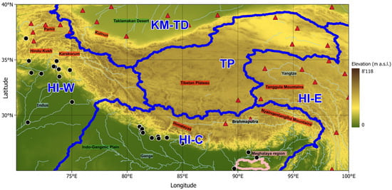
Figure 1. The study region covers latitudes 25–40° N and longitudes 70–100° E. Red labels indicate the main mountain ranges, blue labels indicate the rivers, green labels indicate areas of low orographic complexity, and pink labels indicate the Meghalaya region. Dark blue lines show subregions defined according to Section 3.1, while pink lines show Meghalaya’s boundaries. The black dots indicate the Global Runoff Data Center dataset and the red triangles the Copernicus in situ Observations (see Section 2.2.4). Background is elevation from the Alos AW3D30 DEM resampled to 500 m resolution.

Overall, the study region covers approximately 5 million km² and covers a wide variety of topographic features and climates, ranging from some metres above sea level to the tallest peaks in the world, like Mount Everest (8848 m a.s.l.) in the Himalayan chain and the K2 (8611 m a.s.l.) in the Karakorum chain. As shown in Figure 2, about 50% of the study region is over 3000 m a.s.l., with the dominant elevation range being 4500–5000 m a.s.l., representing the Tibetan Plateau, while about 18% of it lies below 250 m a.s.l., due to the Indo-Gangetic Plain. The elevation distribution follows a bimodal pattern, emphasizing the difference between medium-to-high and low elevations. This area significantly influences the Asian monsoon and global atmospheric circulation through its mechanical and thermal effects [27,28].

Figure 2. Elevation distribution of the study region, represented as the percentage of cells within each 250 m elevation band. The elevations are derived from the Alos AW3D30 DEM, resampled to 500 m resolution. Elevations above 6000 m a.s.l. are grouped together.

2.2. Data

Five gridded precipitation datasets are selected to analyze the spatial distribution and temporal evolution of precipitation over the study region. Specifically, these included two reanalysis datasets (ECWMF-ERA5 and HAR, see Section 2.2.1), two rain gauge-based datasets (APHRODITE and GPCC, see Section 2.2.2), and one satellite dataset (PERSIANN-CDR, see Section 2.2.3). Despite the availability of other precipitation datasets covering periods that partially overlap and extend to the present, our analysis focused on the 1983–2007 period, as discharge observations were available from the 1970s to the early 2000s. The dataset selection was primarily based on single-source products rather than multi-source datasets, e.g., IMERG and CHRISP [16,29], in which the contribution of individual error components is more difficult to analyze.

To investigate the reliability of the analyzed precipitation datasets, we used (i) precipitation observational values from the ‘Copernicus Global Land Surface Atmospheric Variables from 1755 to 2020 from Comprehensive In Situ Observations product [30] from the Copernicus Data Store (Section 2.2.4); (ii) runoff values from the Global Runoff Data Centre [31] (Section 2.2.4); and (iii) total evaporation data from ECMWF-ERA5 Land [32].

2.2.1. Reanalysis Datasets

The reanalysis data selected for precipitation were ECMWF-ERA 5 [11,33] and HARv2 (High Asia Refined Analysis) [13], while ERA5 Land was considered for total evaporation (hereinafter evaporation), which is the accumulated amount of water that has evaporated from the Earth’s surface, including a simplified representation of transpiration (from vegetation), into vapour in the air above.

ERA5 is an hourly dataset on a regular latitude–longitude grid at 0.25-degree resolution which was provided by the European Centre for Medium-Range Weather Forecasts (ECMWF) under Copernicus Climate Change Service, and was available from 1940 to the present.

Unlike ERA5, which covers the entire globe, ERA5-Land focuses exclusively on the land surface, providing hourly information with a spatial resolution of 0.1 degrees from 1950 to the present [32,33,34]. ERA5-Land data are developed using the ECMWF land surface model, which is used to downscale meteorological data from ERA5 and incorporates an elevation correction for the near-surface thermodynamic state.

HARv2, High Asia Refined Analysis Version 2, is a regional climate dataset generated within the framework of the CaTeNA project framework (Climatic and Tectonic Natural Hazards in Central Asia). It offers hourly records, as well as daily and monthly records, for the period from 1980 to 2023. It has a spatial resolution of 10 km and was created using the Weather Research and Forecasting (WRF) [35] model using ERA5 reanalysis data as the forcing data.

2.2.2. Gauge-Based Datasets

In terms of gauge-based precipitation data, APHRODITE V1101 [10] and GPCC Full Data Monthly Product Version 2022 datasets [7] were considered.

APHRODITE (Asian Precipitation Highly Resolved Observational Data Integration Towards Evaluation), provided by Hirosaki University, has a 0.25-degree resolution for the 1951–2007 period and covers the High Mountain Asia area (25–40° N and 70–100° E). It is derived from a network of rain gauge stations across Asia and it includes the entire study region. The data originate from meteorological agencies, international research institutions and historical records, including those collected via the Global Telecommunication System (GTS). APHRODITE is also available after 2007 (APHRODITE-2), but we preferred to consider only APHRODITE-1, as the two different datasets were generated with a different algorithm [10].

The Global Precipitation Climatology Centre (GPCC) dataset is operated by Deutscher Wetterdienst (DWD, National Meteorological Service of Germany) on behalf of the World Meteorological Organization (WMO). The GPCC Full Data Monthly Product Version 2022 provides monthly precipitation data from 1891 to 2020 with a spatial resolution of 0.25 degrees. It combines data from over 75.000 rain gauge stations around the world, obtained from national meteorological services and international organizations, as well as data collected by the World Meteorological Organization.

2.2.3. Satellite Datasets

The PERSIANN-CDR (Precipitation Estimation from Remotely Sensed Information using Artificial Neural Networks—Climate Data Record) Version 1 precipitation dataset, developed by the Center for Hydrometeorology & Remote Sensing (CHRS) at the University of California, Irvine (UCI), is available from 1983 to 2021 with a daily temporal resolution and a spatial resolution of 0.25 degrees. It uses satellite-based infrared (IR) and microwave observations to estimate global precipitation, which is then adjusted using the Global Precipitation Climatology Project (GPCP) monthly product at a resolution of 2.5 degrees [17,36,37].

2.2.4. In Situ Observations

The “Copernicus Global Land Surface Atmospheric Variables from 1755 to 2020 from Comprehensive In Situ Observations Dataset” product, which is available on the Copernicus Data Store, provides access to global land surface meteorological observations acquired by a wide range of organizations, including National Meteorological Services. The dataset is available at sub-daily, daily, and monthly resolutions, is standardized and quality-checked, and includes a relevant number of precipitation records. The covered period varies for each station, although most begin after 1950.

The Global Runoff Data Centre (GRDC) is an international data centre run by the World Meteorological Organization. The dataset was established in 1988 and currently represents over 10,000 monitoring sites around the world. Key partners in data acquisition and management programmes include the World Climate Research Programme (WCRP), the Global Climate Observing System (GCOS), and the UNESCO Intergovernmental Hydrological Programme (IHP).

3. Methods

3.1. Gridded Datasets

The spatial distribution of the five selected gridded precipitation datasets was studied by calculating the monthly and annual precipitation normals over the common period (1983–2007) (see Section 4.1). The annual values were calculated from January to December.

Given the complexity and the extent of the study area, it is divided into five sub-regions (shown by the dark blue lines in Figure 1) according to the borders of the catchments included in the HydroBASINS dataset [38] at levels 3 and 4. This division was chosen to capture major hydrological boundaries without excessive fragmentation. In this way, KM-TD (Kulnun Mountanins—Taklamakan Desert) covers the Kunlun Mountains and the southern part of the Taklamakan Desert, whereas HI-W (Himalaya West) includes the Karakoram, Pamir, Hindu Kush, and western Himalayas. HI-C (Himalaya Centre) contains the central and eastern Himalayan ranges, as well as the Indo-Gangetic Plain, HI-E (Himalaya East) covers the Nyainqentanglha and Tanggula mountain ranges, and TP covers the Tibetan Plateau. To delve deeper into the differences reported by the datasets, the ratios of the precipitation annual normals were determined using the GPCC dataset as a reference (Section 4.2). Although GPCC includes fewer stations than APHRODITE, it uses quality-checked series as input [7]. In addition, GPCC provides the number of stations that are available at each grid cell for each month. This information is useful to extract a selection of grid cells where GPCC is obtained using station data measured in the surroundings, lowering uncertainty in its estimations and resulting in a more rigorous evaluation. Therefore, the datasets were also compared considering only the grid cells that, in GPCC, have at least one station for 60% of the study period. In order to compare the interannual variability, the relative annual anomalies were calculated with respect to the 1983–2007 period and their correlation was computed (Section 4.3).

HAR is the only dataset that does not have a spatial resolution of 0.25 degrees and is defined on a regular Lambert Conformal Conic (LCC) projected grid. As a consequence, to make HAR comparable with GPCC, it was upscaled by averaging neighbouring grid cells using an aggregation window whose size was determined from the ratio between the HAR and GPCC spatial resolutions, resulting in a coarser intermediate grid. This intermediate aggregation step ensures a true spatial averaging of HAR precipitation and avoids relying on direct interpolation from the native high-resolution grid, which would smooth spatial variability without conserving the native values. Finally, to ensure that the resulting HAR grid is spatially aligned with the GPCC grid, a resampling bilinear algorithm was applied [39].

3.2. Stations

To further evaluate the accuracy of the selected precipitation datasets, a point-based validation was carried out using in situ precipitation measurements from the Copernicus dataset (Section 2.2.4). This dataset includes 111 stations distributed across the study area covering the period 1983–2007. To ensure adequate temporal coverage while maintaining spatial representativeness, the analysis only considered stations with at least five years of available data. After applying this selection, the station-based comparison used a reduced subset of 31 stations.

For each selected station and for the corresponding cell of each gridded dataset, annual mean bias (MB) values were computed as the difference between the 1983–2007 gridded precipitation annual normal and the corresponding value from the station observation. Additionally, the standard deviation (SD) of the mean biases was computed to assess the spatial variability of dataset performance. Finally, the mean absolute bias (MAB) was included to evaluate the average magnitude of the bias, regardless of its sign.

Moreover, in order to assess the comparability of the station network and the gridded dataset, the elevation of each station was extracted using the ALOS AW3D30 digital elevation model (DEM) and compared to the elevation of the cell where the station is located. The latter represents the grid cell elevations, estimated from geopotential height in ERA5, from static topography in HAR, and from a DEM in the case of PERSIANN-CDR. The correlation between station and grid elevations using Spearman’s rank correlation coefficient, the mean elevation difference (MELD), and the absolute elevation difference (AELD) were then calculated.

Finally, to assess the relationship between precipitation bias and elevation or terrain complexity we defined and evaluated two parameters—the mean elevation (MEL) and the local terrain complexity (LTC)—which are, respectively, the mean elevation and the standard deviation of the grid cells of the ALOS AW3D30 digital elevation model (DEM), averaged over a 500 m grid box that falls inside each cell of each precipitation dataset. A non-parametric Mann–Kendall test [40,41] was then applied to detect the presence of monotonic trends in the bias values as a function of the two topographic metrics.

3.3. River Discharges

To analyze the reasons underlying the differences observed between the selected precipitation datasets in detail, we also used the information available from the GRDC dataset (Section 2.2.4), which provides annual averages of measured river discharges. Using geoprocessing tools (r.watershed and r.stream.basins in QGIS) applied to a digital elevation model (AW3D30 DEM at 30-metre resolution), it is possible to delineate the upstream catchment area for each discharge station.

For each catchment and for each gridded dataset, the mean annual cumulative precipitation over the same period of the discharge data was calculated considering the grid cells falling inside the considered catchment. As some precipitation datasets do not cover the entire discharge calculation period, a scaling factor was calculated using the ERA5 precipitation dataset, allowing the precipitation to be adjusted to match the time span of the discharge data. The scaling factor was computed by assuming a constant ratio between ERA5 and each of the other datasets.

Then, to estimate a simulated discharge ( $Q_{simulated}$ expressed in $\frac{{\mathrm{m}}^3}{\mathrm{year}}$) on an annual scale, the evaporation dataset from ERA5-Land was used, according to the following equation:

$$Q_{simulated}=P-E$$

(1)

where P is the mean annual precipitation over the catchment for each dataset and for the same period of the discharge data, while E is the corresponding mean annual evaporation. Uncertainties in absolute values of terrestrial evapotranspiration were reported and are related to uncertainties in precipitation forcing [42]. In addition, differences in the estimation and partitioning of evapotranspiration components (e.g., soil evaporation and plant transpiration) can lead to substantial discrepancies among ET products, further increasing uncertainty, particularly in complex environments [43]. To date, no dedicated evaluation of ERA5-Land total evaporation exists for High Mountain Asia, mainly due to the absence of spatially and temporally consistent in situ ET observations. Despite its acknowledged uncertainties, ERA5-Land represents one of the most suitable evaporation datasets for this study because it provides spatially complete and temporally homogeneous estimates.

On an annual basis, we close the catchment water balance with Q ≈ P − E, implicitly assuming that changes in storage (ΔS) average out over a long-time window [44]. Only catchments with more than 5 years of flow measurement were selected from the GRDC. However, in glaciated catchments, part of the runoff may originate from long-term glacier storage, resulting in a non-zero storage term [45]. This is why we chose a glacier cover threshold to exclude catchments where glacier melting could significantly impact runoff. This value is based on the findings of [46], who discovered that in five major catchments of the Tibetan Plateau with glacier coverage between 0.1% and 1.6%, glacier melt contributes less than 5% of the annual runoff. However, catchments with glacier cover between 1.6% and 5% are primarily located in the western Himalaya region (including the Karakoram range in our area definition). It is well established that this region has not experienced significant glacier loss due to the Karakoram Anomaly [47]. Similarly, in western Nepal, glacier mass loss (−0.24 ± 0.11 m.w.a⁻¹) was limited during the 1974–2000 period [48]. We therefore set the glacier cover threshold to 5%.

The number of catchments considered after the application of this threshold is 26, where the area covered by glacier was calculated based on the Randolph Glacier Inventory V7 (2023).

To analyze the performance of the Q_simulated values (Equation (1)) for each precipitation dataset with respect to the measured ones, the Mean Absolute Bias normalized by the area of the catchment (MABN expressed in mm/year), the Percentual Bias normalized by the observed discharge (PBIAS), the Kling–Gupta Efficiency (KGE; [49]), and Spearman’s rank correlation coefficient were calculated.

The MABN quantifies the magnitude of the error between simulated and observed discharge for each catchment and dataset, normalizing the result by the catchment area. This allows for comparison across catchments of different sizes, making it a more consistent and interpretable indicator for visualizing and evaluating the spatial variability of model performance.

The PBIAS measures the average tendency of Q_simulated to overestimate or underestimate Q_observed normalized by the observed discharge value and expressed as a percentage.

The Kling–Gupta Efficiency (KGE) measures how well the model reproduces the observed discharge, combining information about the correlation, the variability, and bias (see Equations (2) and (3)). Values close to 1 indicate a highly accurate model. Although the KGE is commonly used to assess the temporal performance of hydrological models, in this study we applied it across all catchments as a single set of observed and simulated discharge values for each dataset. This is because we analyzed the GRDC-Catalogue that provides long-term mean annual discharge for each catchment.

$$KGE=1-\sqrt{{(r-1)}^2+{(\alpha -1)}^2+{(\beta -1)}^2}$$

(2)

In this context, r is the Pearson correlation coefficient between observed and simulated mean annual discharge across catchments, α is the ratio between the standard deviations (σ) of simulated and observed discharge values across catchments, and β is the ratio between the mean simulated and mean observed discharge (μ) across all catchments, representing the overall bias.

$$\mathrm{K}\mathrm{G}\mathrm{E}=1-\sqrt{{(r-1)}^2+{(\frac{{\sigma }_{\mathrm{s}\mathrm{i}\mathrm{m}}}{{\sigma }_{\mathrm{o}\mathrm{b}\mathrm{s}}}-1)}^2+{(\frac{{\mu }_{\mathrm{s}\mathrm{i}\mathrm{m}}}{{\mu }_{\mathrm{o}\mathrm{b}\mathrm{s}}}-1)}^2}$$

(3)

The PBIAS_dataset (Equation (4)) differs from PBIAS, which computes the percent bias individually for each catchment. In Equation (4), the total bias is calculated as the ratio between the sum of the differences and the sum of the observed discharge across all catchments (n). As a result, catchments with higher discharge have a stronger influence on the final value. This aggregated formulation was used to obtain a comparable bias indicator across datasets.

$${PBIAS}_{dataset}=\frac{{\sum }_{i=1}^n({Q_{simulated}}_i-{Q_{observed}}_i)}{{\sum }_{i=1}^n{Q_{observed}}_i}\times 100$$

(4)

Similarly, the Mean Absolute Bias Normalized by Area (${MABN}_{dataset}$) is computed as the ratio between the total absolute error and the total area of the catchments.

$${MABN}_{dataset}=\frac{{\sum }_{i=1}^n|{Q_{simulated}}_i-{Q_{observed}}_i|}{{\sum }_{i=1}^n{A_{catchment}}_i}$$

(5)

The Spearman coefficient is used instead of the Pearson coefficient to account for possible nonlinear relationships between simulated and observed discharge, and to reduce the influence of outliers across catchments of varying characteristics.

Finally, to compare the observed and simulated discharge values in more detail, a hydrological coefficient is introduced, defined as follows:

$$\rho =\frac{Q_{observed}}{Q_{simulated}}=\frac{Q_{observed}}{P-E}$$

(6)

A value of ρ = 1 indicates an ideal agreement between simulated and observed discharge, while values lower than 1 indicate that P − E exceeds the observed runoff, suggesting an overestimation of precipitation or an underestimated of evaporation. On the contrary, values greater than 1 could be due to an underestimation of precipitation or an overestimation of evaporation. In this analysis, evaporation is coherent across all datasets, because it is derived from ERA5-Land, isolating the effect of precipitation differences on ρ.

After calculating ρ for all catchments, an area-weighted average of ρ is computed for each dataset as follows:

$${\rho }_{mean}=\frac{{\sum }_{i=1}^n{\rho }_i\ast A_i}{{\sum }_{i=1}^n{A}_i}$$

(7)

where ρ_i is the value of the i-catchment A_i is the corresponding catchment area, and n is the number of catchments.

4. Results

4.1. Spatial Distribution of the 1983–2007 Gridded Annual Precipitation Normals

Figure 3 shows the spatial distribution of annual precipitation normals for the period 1983–2007 for all the datasets considered.

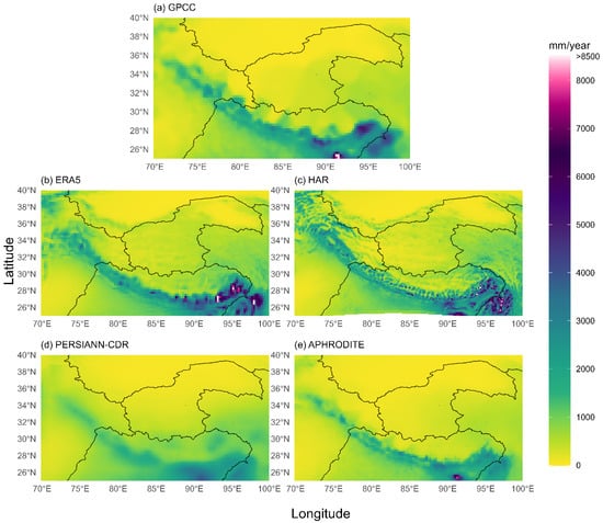
Figure 3. Annual precipitation climatology (1983–2007) over the study area for the different datasets: (a) GPCC, (b) ERA5, (c) HAR, (d) PERSIANN-CDR, and (e) APHRODITE. The division of the five sub-regions (defined according to Section 3.1) is also shown with a black line.

While all the datasets show higher values over the Himalayas and the Karakoram chain, higher values in high-elevation cells compared to lower-elevation cells in the surrounding areas are evident only if the reanalysis datasets are considered. ERA5 and HAR are the only datasets that clearly distinguish between the higher values reported in the Kunlun chain and the Tibetan Plateau and the lower values reported in the Taklamakan Desert. In these datasets, the influence of elevation on precipitation is also particularly evident in the Himalayas and the Karakorum chain. Conversely, PERSIANN-CDR appears to be the least capable of reproducing the dependence of precipitation on orography.

GPCC estimates a highly localized maximum of 9105 mm/year in the Meghalaya region (25–26 E; 90–92 N), a mountainous area in north-eastern India known for its extreme orographic rainfall. This region is home to Mawsynram and Cherrapunji, two of the wettest villages on Earth [50]. This value is also reproduced by the other rain gauge-based dataset: APHRODITE, albeit with a slightly lower estimate of 7747 mm/year, as well as by PERSIANN-CDR, which reports a value of around 4000 mm/year. In ERA5, the peak in this area is less visible, with the highest values reported slightly to the east between the end of the Himalayan chain and the Nyainqentanglha mountains reaching values of around 12,400 mm/year. HAR provides a similar picture with more spatial detail due to its higher spatial resolution, reporting a maximum value of approximately 12,640 mm/year.

The KM-TD subregion shows average annual mean normal values ranging from 69.1 mm for GPCC to 209.9 mm for HAR (Table 1). The differences between the datasets are even more evident when focusing on the maximum values in the subregion, which range from 393.8 mm for PERSIANN-CDR to 2406.0 mm for HAR. The agreement is much better when focusing on the annual cycle (Figure 4). GPCC shows the most pronounced seasonality, with a minimum of 1.5% of the annual cumulative value in November and a maximum of 20.8% in July. By contrast, HAR shows a less pronounced seasonality, with a minimum of about 3.4% of the annual cumulative value in January and a maximum of 15.5% in July. The other datasets exhibit intermediate behaviour between GPCC and HAR.

Table 1. Maximum, minimum, and average annual cumulated precipitation value (mm) for each dataset and sub-region (defined according to Section 3.1).

Dataset	Min	Max	Mean	Area
GPCC	18.7	414.1	69.1	KM-TD
HAR	26.6	2406.0	209.9	KM-TD
ERA5	19.8	1399.5	196.2	KM-TD
PERSIANN	35.9	393.8	100.5	KM-TD
APHRODITE	29.4	409.1	78.1	KM-TD
GPCC	36.5	2648.8	476.3	HI-W
HAR	66.6	4302.6	768.7	HI-W
ERA5	129.4	3651.1	682.8	HI-W
PERSIANN	171.6	1276.1	489.2	HI-W
APHRODITE	83.2	2637.1	373.5	HI-W
GPCC	129.6	9105.4	1325.8	HI-C
HAR	179.9	12,675.5	1507.8	HI-C
ERA5	283.5	12,404.4	1555.3	HI-C
PERSIANN	442.7	3954.7	1279.9	HI-C
APHRODITE	157.1	7747.3	1020.4	HI-C
GPCC	108.7	4159.5	847.1	HI-E
HAR	251.8	12,587.5	1413.7	HI-E
ERA5	286.5	8895.2	1310.7	HI-E
PERSIANN	137.4	3062.9	906.6	HI-E
APHRODITE	148.7	3461.4	695.1	HI-E
GPCC	16.0	926.6	170.5	TP
HAR	32.2	1115.1	316.1	TP
ERA5	33.5	778.3	340.2	TP
PERSIANN	48.8	925.3	232.7	TP
APHRODITE	23.4	443.1	160.6	TP

Figure 4. The percentage of monthly cumulative precipitation (1983–2007) relative to the annual total is shown for each subregion (defined according to Section 3.1) and dataset. The gauge-based datasets (APHRODITE and GPCC) are shown in purple and blue; the reanalysis datasets (HAR and ERA5) are shown in red and orange; and the satellite-based dataset (PERSIANN-CDR) is shown in green.

The TP subregion shows average annual mean normal values ranging from 60.6 mm for APHRODITE to 340.2 mm for ERA5 (Table 1). As for the KM-TD subregion, the differences between the datasets are particularly evident when focusing on the highest values, which range from 443.1 mm for APHRODITE to 1115.1 mm for HAR. The annual cycle (Figure 4) exhibits a similar seasonality to that observed in the KM-TD subregion. All datasets concur that winter is the driest season and summer the wettest, whereas the peak occurs in July for all datasets (24.1 ± 0.8% of the annual cumulated value) except for APHRODITE, which shifts it to August. The dataset that shows the maximum difference between the minimum value (0.62% of the annual cumulated value in January) and the maximum value (25.8% of the annual cumulated value in July) is GPCC.

Moving to the HI-E sub-region, the average annual mean normal values range from 695.1 mm for APHRODITE and 1413.7 mm for HAR (Table 1). HAR and ERA5 report the highest values (12,587.5 mm and 8895.2 mm, respectively) due to their ability to reproduce the dependence of precipitation on elevation, particularly in the southern part of the study region where the Himalayan mountain range ends. Consistent with the KM-TD and TP subregions, the annual cycle (Figure 4) is characterized by a minimum in winter (0.45% of the annual cumulative value for PERSIANN-CDR and 1.5% for HAR, both in December) and a maximum in summer (19.0% for HAR in July and 22.5% for GPCC).

HI-C is the sub-region that exhibits the most complex orography, including the Himalayan region, which is also the mountain range described most coherently by the different datasets. The mean annual normal values range from 1020.4 mm for APHRODITE to 1555.3 mm for ERA5, while the maximum values range from 3954.7 mm for PERSIANN-CDR to 12,675.5 mm for HAR (Table 1). As with the other sub-regions, the annual precipitation cycle (Figure 4) is quite similar between the datasets, with a minimum in winter (0.7% of the annual cumulative value for PERSIANN-CDR and 4.5% for GPCC in December) and a maximum in summer (21.3% for APHRODITE and 24.0% for GPCC in July).

Finally, the HI-W sub-region, including the remainder of the Himalayan and Karakoram chains, exhibits mean annual normal values ranging from 373.5 mm for APHRODITE to 768.7 mm for HAR, while the maximum value range from 1276.1 mm for PERSIANN-CDR to 4302.6 mm for HAR (Table 1). Unlike the other sub-regions, HI-W exhibits a unique precipitation pattern with two seasonal peaks: one in March at 11.2% of the annual cumulative value, and another in July at 20.4%. HAR is the dataset that shows the least pronounced annual cycle compared to the others (Figure 4).

4.2. Ratios Between the Annual Normals of the Datasets and the Corresponding GPCC Values

Figure 5 shows the ratios between the grid cells annual normal values of ERA5, HAR, PERSIANN-CDR, and APHRODITE datasets and the corresponding values of the GPCC dataset for the entire area and for grid cells with observations only (see Section 3.1). Figure 6 shows boxplots of the values of all the cells in Figure 5, excluding outliers, with the median used for evaluation instead of the mean because it is less sensitive to outliers.

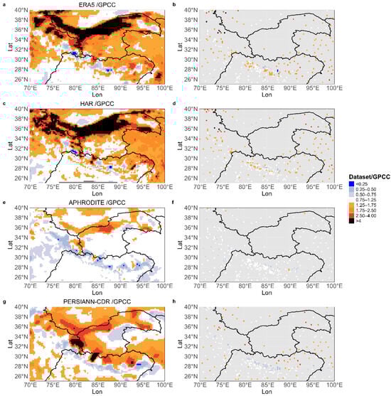
Figure 5. Annual cumulative precipitation ratios between the datasets and GPCC. The results for the entire study area are presented in panels (a,c,e,g), which show the ERA5, HAR, APHRODITE, and PERSIANN results, respectively. The results for grid cells with at least one weather station present for 60% of the GPCC interpolation period are shown in panels (b,d,f,h) (ERA5, HAR, APHRODITE, and PERSIANN-CDR, respectively).

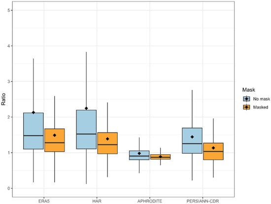
Figure 6. Distribution of the annual cumulated precipitation ratios between the datasets (ERA5, HAR, APHRODITE and PERSIANN-CDR) and GPCC over the entire area. The ‘No mask’ category, shown in light blue, represents the variability of all the grid cells contained in the study area (first column of Figure 5). The ‘Masked’ category, shown in orange, represents the variability of the grid cells with at least one weather station present for 60% of the period used by GPCC to interpolate precipitation (second column of Figure 5). The rhombus indicates the mean value of the ratios, while the whiskers indicate the data range excluding outliers. For visual clarity, outliers are excluded.

ERA5 (Figure 5a,b) generally overestimates precipitation compared to GPCC across the entire domain, particularly in high-elevation regions such as the Kunlun Mountains (KM-TD) and the Tibetan Plateau (TP), where the mean ratios are 2.9 and 3.2, respectively. These large discrepancies are likely related to differences in the representation of precipitation gradients, as well as to the fact that the GPCC dataset does not include any stations in many areas. Moreover, given that the KM-TD region is particularly dry, even small absolute errors can lead to significant deviations. Conversely, higher agreement is found where the orography is less complex, such as in the Indo-Ganges plain. The region with the highest level of agreement is HI-C, with a mean ratio of 1.2.

Considering only grid cells with station coverage increases the overall agreement between the ERA5 and the GPCC datasets. Notably, the HI-C area exhibits two distinct bands across the Himalayan range: one with underestimation (where the ratio is less than 1) and one with overestimation. The mean ratio decreases from 3.2 to 2.2 in the TP area and from 2.9 to 2.0 in the KM-TD area. Furthermore, in the HI-W and HI-E regions, the level of agreement increases, with the mean ratio decreasing from 1.9 to 1.7 in HI-W. Conversely, the average ratio increases from 1.6 to 1.7 in HI-E. This may be because the GPCC-covered cells selected in HI-E have particularly high local ratios, often exceeding 2, which increases the average after masking.

Figure 6 confirms the higher values of the ERA5 dataset with respect to those of the GPCC dataset. The median of the ratios across the entire study area is 1.5 when all cells are considered, whereas it decreases to 1.3 when only the grid cells with observations are considered, indicating an improvement in the dataset performance when selecting cells with stations. Furthermore, the lower whisker remains comparable, while the upper whisker is reduced.

The HAR dataset (Figure 5c,d) exhibits spatial patterns that are comparable to those of the ERA5 dataset. It overestimates precipitation in most areas where GPCC lacks station coverage, with a mean ratio greater than 3 in the Tibetan Plateau (TP) and in the KM-TD region. The region with the highest level of agreement is HI-C with a mean ratio of 1.2.

When the analysis is limited to cells with available GPCC stations, the over- and underestimation characteristics that are clearly visible in ERA5 also appear in HAR, albeit less pronouncedly. This may be attributed to the higher spatial resolution of HAR, which enables it to better resolve topographic gradients. The mean errors in TP and KM-TD decrease from 3.0 to 1.9 and from 3.4 to 1.5, respectively. This indicates the greater reduction than that seen in ERA5, suggesting that even when HAR is scaled up, it remains closer to the GPCC reference values. HI-C remains the region with the ratio closest to 1, decreasing from 1.2 to 1.1. As with ERA5, the HI-W and HI-E regions also exhibit intermediate behaviour between TP, KM-TD, and HI-C for HAR. The mean ratio decreases from 2.0 to 1.6 in HI-W and from 1.9 to 1.8 in HI-E.

Figure 6 provides evidence that the overestimation of the HAR dataset compared to the GPCC dataset is similar to that already observed for the ERA5 dataset. In this case, however, the reduction in the overestimation for the grid cells covered by the stations is slightly more evident.

When considering APHRODITE (Figure 5e,f), unlike the reanalysis datasets, underestimation is generally observed compared to GPCC, except in the KM-TD region and the inner part of the Tibetan Plateau (TP), where mean ratios of 1.2 and 1.1 are observed, respectively. The local minimum occurs in the HI-C area, with a mean value of 0.8.

When considering only grid cells with GPCC stations, the underestimation remains dominant, albeit less intense, with a mean ratio of 0.9 in the HI-C region, where station density is higher. Even though both APHRODITE and GPCC are gridded observed data, this behaviour may be linked to differences in the spatial interpolation algorithm and the station network used. On average, the KM-TD and TP regions are the only ones with ratios greater than 1, with mean values decreasing from 1.2 to 1.0 and from 1.1 to 1.0, respectively, after masking. HI-W and HI-E exhibit intermediate behaviour between HI-C, which shows the strongest underestimation, and KM-TD, which shows the strongest overestimation.

Figure 6 confirms that APHRODITE is the dataset with the smallest differences in the unmasked column compared to GPCC. When considering only the grid cells with observations, the median ratio decreases however from 0.9 to 0.8, indicating a widespread underestimation relative to GPCC, even though the difference between the first and third quartile decreases, suggesting that the observed differences have higher spatial coherence.

Figure 5g shows that the PERSIANN-CDR dataset tends to overestimate precipitation relative to the GPCC dataset, with a ratio that is consistently greater than one across all regions. The largest values occur in TP (the mean ratio is 1.7), followed by KM-TD (1.6) and HI-W (1.4). The lowest ratio is found in HI-C, where PERSIANN-CDR is closer to GPCC, with a mean ratio of 1.25. This spatial pattern divides the domain into three zones: the southern area with moderate overestimation (HI-E), the central zone with a good agreement (HI-C), and the northern zone with a strong overestimation (KM-TD and TP).

When only grid cells with GPCC stations are considered (Figure 5h), the agreement is much better. The average ratio in HI-C drops from 1.2 to 1.0, indicating excellent agreement where ground observations are available. Similarly, the average ratios in HI-W and KM-TD decrease from 1.4 to 1.1 and 1.6 to 1.4, respectively, suggesting a substantial reduction in bias when considering observed areas. Conversely, the average ratio in TP rises slightly from 1.7 to 1.8, likely due to the inclusion of high-ratio cells in the masked dataset. As with the other regions, the ratio in HI-E increases slightly from 1.2 to 1.3. Overall, the masked analysis confirms that HI-C remains the most consistent region, whereas PERSIANN-CDR tends to overestimate precipitation more strongly in the northern parts of the domain, especially in TP and KM-TD.

PERSIANN-CDR exhibits intermediate behaviour between the reanalysis datasets and the gauge-based APHRODITE dataset when all grid cells are considered. However. when only the masked cells are considered, the median error decreases from 1.2 to 1.0, making PERSIANN-CDR the dataset closest to GPCC.

4.3. Interannual Variability of the 1983–2007 Gridded Precipitation Dataset

Figure 7 shows the mean subregional relative anomaly series for ERA5, HAR, APHRODITE, and PERSIANN-CDR yearly precipitation in the 1983–2007 period, together with the corresponding series obtained using the GPCC dataset. Additionally, the spatial distribution of the correlation between the grid cell yearly precipitation anomaly series for ERA5, HAR, APHRODITE, and PERSIANN-CDR and the corresponding GPCC series is shown. All the datasets show a good correlation with GPCC when focusing on the subregional average series, whereas the agreement is less evident when focusing on the grid cell series, which also show negative correlations in some areas.

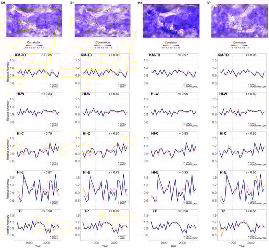
Figure 7. Comparison of the interannual variability of mean precipitation across the study area, based on different datasets. Each panel (a–d) shows the results for one dataset: (a) ERA5, (b) HAR, (c) APHRODITE, and (d) PERSIANN-CDR. The line plots display the annual mean relative precipitation anomalies for each sub-region, comparing the selected dataset (orange) with GPCC (blue). The maps show the spatial distribution of the correlation coefficients between the series of GPCC and those of the corresponding dataset over the entire study period (1983–2007). The r values reported in the regional graphs represent the Pearson correlation coefficient between the two anomaly series.

APHRODITE shows the highest correlation with GPCC, both for the subregional average yearly anomaly series (correlation coefficients are between 0.85 (HI-C) and 0.97 (KM-TD)) and for the corresponding grid cell series.

PERSIANN-CDR shows a lower correlation with GPCC compared to APHRODITE. The area with the highest correlation in the subregional average yearly anomaly series is KM-TD, in agreement with APHRODITE, reaching a value of 0.96. The area with the lowest correlation is HI-E with a value of 0.80. Additionally, the reanalysis datasets show lower correlation with GPCC compared to APHRODITE.

4.4. Comparisons with Ground-Based Weather Stations

To gain a better understanding of the differences observed in the analyzed datasets, they were compared with station observations (Section 3.2). However, as GPCC and APHRODITE are gridded observational datasets, they were excluded from this analysis. Validation therefore focused on ERA5 and HAR, whose precipitation estimates are independent of local gauge data, as well as PERSIANN-CDR. Although PERSIANN-CDR is not fully independent due to the monthly bias correction applied using GPCP at a 2.5-degree resolution, it was included because this correction is applied at a coarse spatial scale and is therefore unlikely to affect local-scale validation.

As shown in Table 2, PERSIANN-CDR demonstrates the greatest agreement with the observations: it has a mean bias of +114.4 mm; the lowest spatial variability (SD = 146.0 mm); and the lowest mean absolute bias (MAB = 139.6 mm). This indicates a low average error and great consistency between the dataset and the measured values. HAR exhibits an intermediate pattern, with a higher mean bias (+180.7 mm) and greater variability in errors across the region (SD = 179.0 mm, MAB = 194.8 mm). ERA5 exhibits the worst performance in this comparison, with the highest mean bias (+320.5 mm) and the greatest variability among stations (SD = 425.0 mm, MAB = 327.0 mm).

Table 2. Mean Bias (MB) between the annual cumulated precipitation values between the considered gridded dataset (HAR, PERSIANN and ERA5) and the station observations. Standard Deviation (SD) and Mean Absolute Bias (MAB) between annual cumulated values from weather station and datasets.

Dataset	MB	SD	MAB
HAR	180.7	179.0	194.8
PERSIANN	114.4	146.0	139.6
ERA5	320.5	425.0	327.6

These results, however, should be considered carefully, as some of the bias may be due to errors in station observations or to a low ability of the stations to capture the average precipitation in grid cells. This issue is particularly relevant as stations are often located in dry valleys and at elevations that do not correspond to the mean elevation of the grid cell. While stations provide precipitation at a single point and elevation, gridded datasets represent the spatial average over the entire cell, which can introduce substantial mismatches in complex topography.

To explore these aspects, a two-step analysis was carried out. First, the elevation of each station was compared to the mean elevation of the corresponding grid cell. The mean error for HAR is 264.0 m, which is the lowest of the three datasets and is likely due to its finer spatial resolution. Next is PERSIANN-CDR, with a mean error of 350.2 m, followed by ERA5, which shows a mean difference of 368.5 m between station elevation and the elevation of the corresponding grid cell. A correlation test was then performed between the station elevation and the mean elevation of the grid, and the results show a high correlation for all datasets. This confirms that, despite the elevation mismatch, the selected grid cell can be considered reasonably representative of the corresponding stations. As expected, the correlation is slightly higher for the dataset with a finer spatial resolution (0.98 for HAR) than for those with a coarser resolution (0.96 for ERA5 and PERSIANN-CDR).

Elevation mismatch could influence precipitation bias in all three datasets. In fact, when the MB and the mean elevation differences in altitude (MELD) are compared, a positive significant linear trend is found, underlining the increasing bias between gridded datasets and station observations as the difference in elevation increases. This effect is stronger for ERA5, which reports an increase of 0.47 mm/m (p-value < 0.01), followed by HAR (approximately 0.36 mm/m, p-value < 0.05) and PERSIANN-CDR (approximately 0.23 mm/m, p-value < 0.01). Additionally, a linear relationship is also confirmed when the absolute elevation difference (AELD) is considered. This shows that the direction and magnitude of elevation mismatch both contribute to the error. ERA5 again shows the highest slope (approximately 0.61 mm/m, p-value < 0.01), followed by HAR (approximately 0.41 mm/m, p-value < 0.05) and PERSIANN-CDR (approximately 0.26 mm/m, p-value < 0.01).

To evaluate the extent to which the observed bias may be due to the area’s complexity, the mean bias (MB) is assessed against the topographic characteristics of mean elevation and local topography complexity (MEL and LTC, respectively; see Section 3.2) of the cell in which the station is located. To achieve this, a Mann–Kendall trend test and Theil–Sen slope were applied to each dataset, and the results are presented in Table 3.

Table 3. Results of the Mann–Kendall trend test and Theil–Sen slope between mean bias (MB) and MEL (mean elevation), and between MB and LTC (topographic complexity). p-values < 0.01 and corresponding slope values are in bold.

Dataset	MEL	LTC
HAR	+0.05	+0.73
ERA5	+	+0.73
PERSIANN-CDR	+	+0.28

A significant positive trend of the MB with MEL was only detected for HAR, indicating that the bias increases at a rate of +0.05 mm/m in higher-altitude areas. In contrast, neither ERA5 nor PERSIANN-CDR show significant trends with mean elevation, suggesting that their over- or underestimation is not systematically influenced by the MEL of the cell in which the station is located.

As for LTC, which is expressed as the standard deviation of elevation within the grid cell, a positive trend is observed for all datasets, highlighting a tendency for increased bias in more complex areas. HAR and ERA5 show the same rate of +0.73 mm/m, while PERSIANN-CDR shows a rate of about +0.28 mm/m, with p-values < 0.01 for all three datasets.

4.5. Comparison with Discharge Measurements

To delve deeper into the differences observed between the analyzed datasets, we calculated the expected yearly average discharge values for the catchments with discharge measurements using precipitation (P) and total evaporation (E) data (Section 3.3), and we compared them with the values of the GRDC dataset.

The results show that some of them have negative P-E values (see Table 4), due to total evaporation being higher than precipitation. We eliminated these from the subsequent analysis to ensure comparability across datasets. This decreased the number of catchments considered to 23.

Table 4. Discharge estimates (Q_dataset) and corresponding observed discharge (Q_GRDC), expressed in m³/s for catchments where at least one estimated discharge value was negative. The catchment area (A_catchment) is expressed in km².

Catchment	QGRDC	QHAR	QERA5	QAPHRODITE	QGPCC	QPERSIANN	Acatchment
GURRIALA	25.9	32.9	15.7	−2.04	11.9	−9.7	3107.4
JHANSI POST	3.8	7.4	−7.9	−24.0	−36.9	−18.5	1818.4
NEAR KOTLI	130.3	112.6	79.3	−6.9	45.8	27.9	3751.6

Figure 8 summarizes the accuracy of the simulated discharges derived from the five gridded precipitation datasets by evaluating their mean annual bias (MABN) and percent bias (PBIAS) across all catchments.

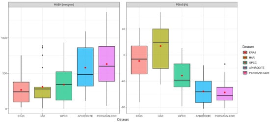
Figure 8. The boxplot shows the distribution of the normalized mean absolute bias (MABN) and percent bias (PBIAS) for all catchments in each dataset (ERA5 in pink, HAR in dark green, GPCC in light green, APHRODITE in blue, and PERSIANN-CDR in fuchsia). The mean is represented by a red dot; the line indicates the median; and the grey dots show the outliers (values that fall outside the typical range, which is defined as 1.5 times the interquartile range below the first quartile or above the third quartile). The whiskers indicate the data range excluding outliers.

ERA5, on one side, displays MABN values ranging from 0 to 750 mm/year, with a mean of 267 mm/year indicated by the red dot in the figure, while on the other side it shows PBIAS values ranging between −75% and 40%, with a mean of −9.2%. HAR has the lowest MABN variability (difference between the first and third interquartile) compared to the other datasets, although the presence of four outliers raises the mean error to 310 mm/year; however, this is only higher than the ERA5 error. The PBIAS values range from −50% to 70%, with a mean of +13.2% and overestimation of the simulated streamflow compared to the underestimation of ERA5.

When moving from the reanalysis dataset to the gridded observed datasets, GPCC exhibits a comparable MABN value (341 mm/year) to that observed for the reanalysis datasets, even though this is the result of more widespread values (between 0 and 900 mm/year). This suggests higher variability in the differences between simulated and observed values across different catchments. The PBIAS range spans from −80% to 20%, even though the mean value is higher, at −31.2%, indicating a greater underestimation of simulated streamflow. The second gauge-based dataset, APHRODITE, shows greater MABN values than GPCC, ranging from 100 to 1100 mm per year. This results in a higher mean value (580 mm per year) than that found for GPCC and the two reanalysis datasets. The PBIAS shows a comparable range across the different catchments (−85% to −17%), although the mean value (−55.8%) indicates stronger underestimation of simulated discharge than the previous datasets.

Lastly, the satellite-based PERSIANN-CDR dataset exhibits the greatest variability in MABN, ranging from 10 to 1300 mm/year, with an average of 631 mm/year. The mean PBIAS value of −57.3% is consistent with that of APHRODITE and confirms a marked underestimation of the simulated discharge.

In order to obtain an overall view of the behaviour of the different datasets, their performance was also evaluated treating all catchments as a single system and calculating the corresponding PBIAS_basin and MABN_basin (Equations (4) and (5)).

According to Table 5, ERA5 exhibits the best overall performance, with the lowest PBIAS_basin (−7.8%), the highest KGE (0.90), and the lowest MABN_basin (115.0 mm/year). It has a high Spearman correlation (0.97), indicating a strong monotonic relationship between estimated and observed values. Notably, MABN_basin mean for ERA5 is lower than the mean MABN in Figure 8 (267.0 mm/year), which suggests that some of the local differences may compensate for each other when catchments are combined into a single system. Also, HAR performs reasonably well in terms of correlation (Spearman = 0.99) and KGE (0.72), but tends to underestimate discharge overall (PBIAS_basin = −17.7%), in contrast to what is suggested by the positive average PBIAS in Figure 8. This discrepancy is likely due to the influence of outliers, which have a stronger impact when aggregating all catchments as a single system; they occur due to the fact that the underestimation of Q_simulated is not systematic for all the catchments.

Table 5. Metrics for all catchments defined according to Section 3.3: Percent Bias, Kling–Gupta Efficiency, and Mean Absolute Bias Normalized and Spearman’s correlation.

Dataset	PBIASbasin	KGE	MABNbasin	Spearman
HAR	−17.7%	0.71	270.0	0.99
ERA5	−7.84%	0.91	115.0	0.97
GPCC	−43.8.%	0.36	554.0	0.96
PERSIANN	−51.1.%	0.30	645.0	0.97
APHRODITE	−73.1%	−0.04	922.0	0.94

The gauge-based GPCC and the satellite product PERSIANN-CDR show larger negative biases (−43.8% and −51.1%, respectively) and higher absolute errors (554.0 mm/year and 645.0 mm/year) compared to the reanalysis datasets, as shown in Figure 8. While PERSIANN-CDR performance in the aggregated evaluation is consistent with the catchment analysis in Figure 8, GPCC shows a noticeable decline in performance. This is likely due to the fact that GPCC errors are less evenly distributed across catchments, and when aggregated, negative deviations have a stronger influence on the overall PBIAS_basin. In contrast, more balanced local errors (as in ERA5) tend to compensate when catchments are treated as a single system. The KGE values support this interpretation, with GPCC and PERSIANN-CDR showing moderate values (0.36 and 0.30, respectively). Despite the high Spearman correlations, these low KGE scores suggest deficiencies in reproducing the overall variability and bias of observed discharge, reducing their reliability compared to the reanalysis datasets.

APHRODITE performs the worst overall, with the lowest KGE (−0.04), the highest absolute error (MABN_basin = 922.0 mm/year) and the strongest underestimation of simulated discharge (PBIAS_basin = −73.1%). These results are consistent with the result in Figure 8, confirming that APHRODITE underestimates streamflow across most catchments.

Finally, in order to spatially visualize the obtained values, Figure 9 shows the spatial distribution of the ρ coefficient (Equation (6)) for all analyzed catchments.

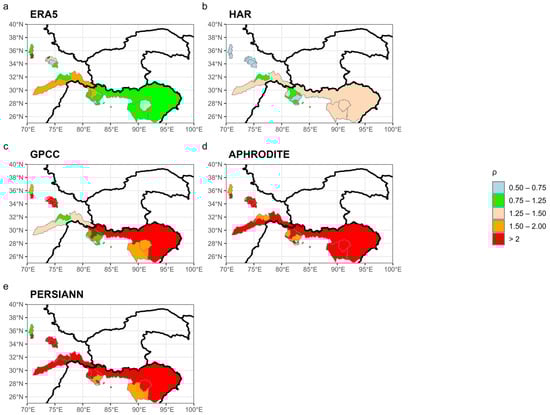
Figure 9. Distribution of the ρ values over the 23 catchments considered. The optimal values range from 0.75 to 1.25 and are shown in green. The results are presented as follows: panel (a) ERA5, (b) HAR, (c) GPCC, (d) APHRODITE, and (e) PERSIANN-CDR.

ERA5 shows that most catchments fall within 0.75 < ρ < 1.50, indicating a generally good agreement between the estimated and observed discharge even if two catchments show ρ < 0.75 and two others ρ > 1.50. Similarly to ERA5, HAR performs well in several central Himalayan catchments (HI-C), where ρ values lie between 0.75 and 1.25. Larger catchments, which in ERA5 are classified in the green or orange categories, now fall into the 1.25–1.50 range, suggesting a slight underestimation of runoff.

The GPCC dataset tends to produce higher ρ values overall, with many catchments exceeding 1.25 and several (particularly in the Karakoram and eastern Himalayas, an area characterized by complex orography and a low number of available stations (see Figure 5) above 1.50. This indicates a widespread underestimation of precipitation. However, some central catchments fall within the 0.75–1.25 range, which is consistent with the performance of ERA5 and HAR.

APHRODITE and PERSIANN-CDR reveal a generalized underestimation of runoff. Almost all catchments show a value of ρ greater than 1.50, and only three catchments in each dataset fall below this threshold. This suggests that, across almost the entire region, the estimated precipitation is insufficient to match the observed discharge, even when evaporation is accounted for.

The average ρ coefficient (ρ_mean) was also calculated for each dataset across all catchments. Consistent with previous observations, ERA5 exhibits the lowest ρ_mean (1.13), indicating the best overall agreement between simulated and observed discharge. HAR has a slightly higher value (ρ_mean = 1.22), suggesting a modest tendency to underestimate discharge. GPCC shows a value of 1.78, indicating widespread underestimation of precipitation across the region. PERSIANN-CDR and APHRODITE display the highest values (2.14 and 3.95, respectively), indicating a very high underestimation of the observed discharge. These results are consistent with the spatial patterns shown in Figure 9 and support the conclusion that reanalysis products (ERA5 and HAR) provide more consistent discharge estimates than gauge-based (APHRODITE and GPCC) and satellite-derived (PERSIANN-CDR) datasets.

5. Discussion

This study provides a comprehensive evaluation of five gridded precipitation datasets (HAR, ERA5, GPCC, APHRODITE, and PERSIANN-CDR) across High Mountain Asia, using both station-based and hydrological validation approaches. The results reveal notable differences in spatial patterns, elevation sensitivity, and hydrological consistency.

Reanalysis datasets (HAR and ERA5) demonstrate the highest ability to capture the complex orographic precipitation gradients, particularly along the Himalayas, Kunlun Mountains, and Tibetan Plateau. This is largely because the influence of the scarcity of observational stations has a more limited influence on the reanalysis datasets than on those that depend directly on the observations. Moreover, the observational stations are often located in dry valleys and they are therefore not able to capture the higher normal values that often characterize the neighbouring areas at higher elevation. In order to investigate the correlation between elevation and precipitation in the study region, we focused on the HAR dataset, because of its higher spatial resolution. Specifically, we considered a box of 25 grid cells centred over each grid cell and we calculated the correlation coefficient between the elevation and the annual normal precipitation. The results (Figure 10) clearly show the link between these variables in most cells of the study region. This link is often only partially captured by rain gauge-based (GPCC, APHRODITE) and satellite-based (PERSIANN-CDR) datasets because of the low number of stations and because they are often located in valleys. These datasets therefore show smoother spatial patterns and tend to underestimate precipitation extremes in orographically driven regions—e.g., the underestimation of Meghalaya rainfall by PERSIANN-CDR. This is consistent with [51], which reported that PERSIANN-CDR systematically underestimates extreme precipitation events, particularly in orographically complex regions, and with [3], which report that high-resolution reanalysis datasets show a similar elevation dependency of precipitation with observations.

Figure 10. Correlation between precipitation and elevation based on 5 × 5 cell-windows cantered around each grid cell (a); cells with correlation coefficient > 0.7 (b).

Despite these differences, all datasets agree on the seasonal cycle of precipitation, with a dry winter and a wet summer across most subregions. The westernmost region (HI-W) shows a distinct bimodal pattern associated with westerly disturbances during winter [52] and the Indian monsoon during the summer months [53]; this signal is captured coherently by all datasets. The winter peak, however, is more strongly represented by HAR compared to the other datasets. This is consistent with the findings of [3], who showed that high-resolution reanalyses such as HAR are better able to capture winter precipitation related to westerly disturbances. Meanwhile, the coarse resolution data show less precipitation because they allow more water vapour to be transported into the Tibetan Plateau, due to lower roughness related to the smoother land surface [54].

Interannual variability analysis highlights the strengths of gauge-based APHRODITE, which shows the highest mean correlation with GPCC anomalies—unsurprising given their shared observational foundation. ERA5 and HAR also correlate well with GPCC but show local discrepancies in areas with sparse station coverage, especially over KM-TD and HI-C. PERSIANN-CDR, while benefiting from GPCP-based bias correction, exhibits heterogeneous behaviour, performing well in some subregions but poorly in others.

When comparing datasets with ground station measurements, PERSIANN-CDR shows lower bias than HAR and ERA5 in terms of mean bias and mean absolute bias, in line with [55,56]. However, this apparent advantage decreases when considering topographic mismatch: reanalysis datasets show a stronger correlation between bias and elevation or terrain complexity, reflecting their sensitivity to grid-cell characteristics. PERSIANN-CDR’s coarser resolution and bias correction reduce this sensitivity but also flatten orographic signals.

To overcome the limitations of point-based validation, we also assessed the datasets against observed river discharge using a catchment-scale water balance approach. This method averages out local mismatches and offers a robust test of the dataset’s hydrological realism. The results show a significant contrast with station-based findings. ERA5 emerges as the most hydrologically consistent dataset, with the lowest catchment-wide bias (−7.8%), smallest absolute error, and highest Kling–Gupta Efficiency (KGE = 0.91). HAR follows closely (KGE = 0.72), though it exhibits slightly more underestimation of the observed discharge in certain catchments. Gauge-based datasets (GPCC, APHRODITE) and PERSIANN-CDR tend to strongly underestimate observed discharges, particularly in remote or glaciated catchments. Their poorer performance likely reflects insufficient representation of orographic precipitation and sparse station networks in mountainous terrain. APHRODITE shows the weakest results overall, with the largest underestimation, confirming its limited applicability in hydrological studies across complex terrain. This ranking is consistent with findings from other studies that applied similar water balance approaches, although in more localized regions [3,18,20,57,58]. These results may be attributed to differences in gauge network density, station selection algorithms, or the bias correction schemes applied. Notably, GPCC includes a correction factor to adjust for gauge under catch, but this adjustment may still be insufficient to fully account for the precipitation losses in high-altitude or complex terrain [21]. The most evident limitation of the datasets = depending on the observations, however, is clearly the extremely low station density in relevant parts of the investigated area.

6. Conclusions

Our results demonstrate that no single precipitation dataset excels across all validation methods.

ERA5 offers the best trade-off between spatial structure, elevation sensitivity, and hydrological consistency. It is the most reliable choice for catchment-scale hydrological modelling over High Mountain Asia.

HAR, with its high spatial resolution, better captures local precipitation gradients and orographic signals, making it especially suitable for studies focusing on mountain processes, despite a slightly higher overall bias.

Gauge-based datasets like GPCC and APHRODITE are useful for point-level climatology and in well-instrumented regions, but their performance deteriorates at high elevations and in data-scarce areas.

PERSIANN-CDR performs well at station locations due to its bias correction scheme but lacks spatial realism and hydrological coherence, particularly in mountainous or glaciated catchments.

We conclude that reanalysis datasets, particularly ERA5 and HAR, are the most suitable for hydrological studies in High Mountain Asia. Their ability to represent orographic gradients and their consistency in reproducing the observed discharge make them robust tools for large-scale applications in data-sparse regions. On the other hand, the well-known problems of reanalysis datasets in correctly capturing long-term precipitation trends [59] suggest that, for studies focusing on climate change, rain gauge stations and datasets based on them are absolutely fundamental.

Recent advances have led to the development of new high-resolution precipitation products over the Tibetan Plateau and surrounding regions, including regional reanalyses and model-based datasets extending closer to the present (e.g., [60,61]). These datasets represent an important step forward for future applications.

In future, we plan to extend the analysis, both increasing the investigated temporal window and considering other datasets, such as IMERG [16], HAR V2 [13], and high-resolution Tibetan Plateau regional reanalysis [60].

References

- Trenberth, K.E.; Dai, A.; Rasmussen, R.M.; Parsons, D.B. The Changing Character of Precipitation. Bull. Am. Meteorol. Soc. 2003, 84, 1205–1217+1161. [Google Scholar] [CrossRef]
- Yao, T.; Bolch, T.; Chen, D.; Gao, J.; Immerzeel, W.; Piao, S.; Su, F.; Thompson, L.; Wada, Y.; Wang, L.; et al. The Imbalance of the Asian Water Tower. Nat. Rev. Earth Environ. 2022, 3, 618–632. [Google Scholar] [CrossRef]
- Sun, H.; Su, F.; He, Z.; Ou, T.; Chen, D.; Li, Z.; Li, Y. Hydrological Evaluation of High-Resolution Precipitation Estimates from the WRF Model in the Third Pole River Basins. J. Hydrometeorol. 2021, 22, 2055–2071. [Google Scholar] [CrossRef]
- Talchabhadel, R.; Karki, R. Assessing Climate Boundary Shifting under Climate Change Scenarios across Nepal. Environ. Monit. Assess. 2019, 191, 520. [Google Scholar] [CrossRef]
- Huffman, G.J.; Adler, R.F.; Morrissey, M.M.; Bolvin, D.T.; Curtis, S.; Joyce, R.; McGavock, B.; Susskind, J. Global Precipitation at One-Degree Daily Resolution from Multisatellite Observations. J. Hydrometeorol. 2001, 2, 36–50. [Google Scholar] [CrossRef]
- Immerzeel, W.W.; Wanders, N.; Lutz, A.F.; Shea, J.M.; Bierkens, M.F.P. Reconciling High-Altitude Precipitation in the Upper Indus Basin with Glacier Mass Balances and Runoff. Hydrol. Earth Syst. Sci. 2015, 19, 4673–4687. [Google Scholar] [CrossRef]
- Schneider, U.; Finger, P.; Meyer-Christoffer, A.; Rustemeier, E.; Ziese, M.; Becker, A. Evaluating the Hydrological Cycle over Land Using the Newly-Corrected Precipitation Climatology from the Global Precipitation Climatology Centre (GPCC). Atmosphere 2017, 8, 52. [Google Scholar] [CrossRef]
- Harris, I.; Jones, P.D.; Osborn, T.J.; Lister, D.H. Updated High-Resolution Grids of Monthly Climatic Observations—The CRU TS3.10 Dataset. Int. J. Climatol. 2014, 34, 623–642. [Google Scholar] [CrossRef]
- Chen, M.; Xie, P.; Janowiak, J.E. Global Land Precipitation: A 50-Yr Monthly Analysis Based on Gauge Observations. J. Hydrometeorol. 2002, 3, 249–266. [Google Scholar] [CrossRef]
- Yatagai, A.; Kamiguchi, K.; Arakawa, O.; Hamada, A.; Yasutomi, N.; Kitoh, A. Aphrodite Constructing a Long-Term Daily Gridded Precipitation Dataset for Asia Based on a Dense Network of Rain Gauges. Bull. Am. Meteorol. Soc. 2012, 93, 1401–1415. [Google Scholar] [CrossRef]
- Hersbach, H.; Bell, B.; Berrisford, P.; Hirahara, S.; Horányi, A.; Muñoz-Sabater, J.; Nicolas, J.; Peubey, C.; Radu, R.; Schepers, D.; et al. The ERA5 Global Reanalysis. Q. J. R. Meteorol. Soc. 2020, 146, 1999–2049. [Google Scholar] [CrossRef]
- Kobayashi, S.; Ota, Y.; Harada, Y.; Ebita, A.; Moriya, M.; Onoda, H.; Onogi, K.; Kamahori, H.; Kobayashi, C.; Endo, H.; et al. The JRA-55 Reanalysis: General Specifications and Basic Characteristics. J. Meteorol. Soc. Jpn. 2015, 93, 5–48. [Google Scholar] [CrossRef]
- Wang, X.; Otto, M.; Scherer, D. Atmospheric Triggering Conditions and Climatic Disposition of Landslides in Kyrgyzstan and Tajikistan at the Beginning of the 21st Century. Nat. Hazards Earth Syst. Sci. 2021, 21, 2125–2144. [Google Scholar] [CrossRef]
- Kummerow, C.; Simpson, J.; Thiele, O.; Barnes, W.; Chang, A.T.C.; Stocker, E.; Adler, R.F.; Hou, A.; Kakar, R.; Wentz, F.; et al. The Status of the Tropical Rainfall Measuring Mission (TRMM) after Two Years in Orbit. J. Appl. Meteorol. 2000, 39, 1965–1982. [Google Scholar] [CrossRef]
- Skofronick-Jackson, G.; Petersen, W.A.; Berg, W.; Kidd, C.; Stocker, E.F.; Kirschbaum, D.B.; Kakar, R.; Braun, S.A.; Huffman, G.J.; Iguchi, T.; et al. The Global Precipitation Measurement (GPM) Mission for Science and Society. Bull. Am. Meteorol. Soc. 2017, 98, 1679–1695. [Google Scholar] [CrossRef] [PubMed]
- Huffman, G.J.; Bolvin, D.T.; Braithwaite, D.; Hsu, K.L.; Joyce, R.J.; Kidd, C.; Nelkin, E.J.; Sorooshian, S.; Stocker, E.F.; Tan, J.; et al. Integrated Multi-Satellite Retrievals for the Global Precipitation Measurement (GPM) Mission (IMERG). In Advances in Global Change Research; Springer: Berlin/Heidelberg, Germany, 2020; Volume 67, pp. 343–353. [Google Scholar]
- Sorooshian, S.; Hsu, K.L.; Gao, X.; Gupta, H.V.; Imam, B.; Braithwaite, D. Evaluation of PERSIANN System Satellite-Based Estimates of Tropical Rainfall. Bull. Am. Meteorol. Soc. 2000, 81, 2035–2046. [Google Scholar] [CrossRef]
- Chen, Y.; Ding, M.; Zhang, G.; Wang, Y.; Li, J. Evaluation of ERA5 Reanalysis Precipitation Data in the Yarlung Zangbo River Basin of the Tibetan Plateau. J. Hydrometeorol. 2023, 24, 1491–1507. [Google Scholar] [CrossRef]
- Sun, H.; Su, F.; Yao, T.; He, Z.; Tang, G.; Huang, J.; Zheng, B.; Meng, F.; Ou, T.; Chen, D. General Overestimation of ERA5 Precipitation in Flow Simulations for High Mountain Asia Basins. Environ. Res. Commun. 2021, 3, 121003. [Google Scholar] [CrossRef]
- Zhang, Y.; Ju, Q.; Zhang, L.; Xu, C.Y.; Lai, X. Evaluation and Hydrological Application of Four Gridded Precipitation Datasets over a Large Southeastern Tibetan Plateau Basin. Remote Sens. 2022, 14, 2936. [Google Scholar] [CrossRef]
- Baudouin, J.-P.; Herzog, M.; Petrie, C.A. Cross-Validating Precipitation Datasets in the Indus River Basin. Hydrol. Earth Syst. Sci. 2020, 24, 427–450. [Google Scholar] [CrossRef]
- Dollan, I.J.; Maina, F.Z.; Kumar, S.V.; Nikolopoulos, E.I.; Maggioni, V. An Assessment of Gridded Precipitation Products over High Mountain Asia. J. Hydrol. Reg. Stud. 2024, 52, 101675. [Google Scholar] [CrossRef]
- Hussain, S.; Song, X.; Ren, G.; Hussain, I.; Han, D.; Zaman, M.H. Evaluation of Gridded Precipitation Data in the Hindu Kush–Karakoram–Himalaya Mountainous Area. Hydrol. Sci. J. 2017, 62, 2393–2405. [Google Scholar] [CrossRef]
- Kanda, N.; Negi, H.S.; Rishi, M.S.; Kumar, A. Performance of Various Gridded Temperature and Precipitation Datasets over Northwest Himalayan Region. Environ. Res. Commun. 2020, 2, 085002. [Google Scholar] [CrossRef]
- Maina, F.Z.; Kumar, S.V. Diverging Trends in Rain-On-Snow Over High Mountain Asia. Earths Future 2023, 11, e2022EF003009. [Google Scholar] [CrossRef]
- Qiu, J. China: The Third Pole. Nature 2008, 454, 393–396. [Google Scholar] [CrossRef]
- Yoon, Y.; Kumar, S.V.; Forman, B.A.; Zaitchik, B.F.; Kwon, Y.; Qian, Y.; Rupper, S.; Maggioni, V.; Houser, P.; Kirschbaum, D.; et al. Evaluating the Uncertainty of Terrestrial Water Budget Components over High Mountain Asia. Front. Earth Sci. 2019, 7, 120. [Google Scholar] [CrossRef]
- Duan, A.; Wu, G. Weakening Trend in the Atmospheric Heat Source over the Tibetan Plateau during Recent Decades Part 1: Observations. J. Clim. 2008, 21, 3149–3164. [Google Scholar] [CrossRef]
- Funk, C.; Peterson, P.; Landsfeld, M.; Pedreros, D.; Verdin, J.; Shukla, S.; Husak, G.; Rowland, J.; Harrison, L.; Hoell, A.; et al. The Climate Hazards Infrared Precipitation with Stations—A New Environmental Record for Monitoring Extremes. Sci. Data 2015, 2, 150066. [Google Scholar] [CrossRef] [PubMed]
- Copernicus Climate Change Service, Climate Data Store, (2021): Global Land Surface Atmospheric Variables from 1755 to Present from Comprehensive in-Situ Observations. Copernicus Climate Change Service (C3S) Climate Data Store (CDS). Available online: https://cds.climate.copernicus.eu/datasets/insitu-observations-surface-land?tab=overview (accessed on 17 July 2024).
- The Global Runoff Data Centre, 56068 Koblenz, Germany. 2020. Available online: https://Grdc.Bafg.de/ (accessed on 13 September 2014).
- Muñoz-Sabater, J.; Dutra, E.; Agustí-Panareda, A.; Albergel, C.; Arduini, G.; Balsamo, G.; Boussetta, S.; Choulga, M.; Harrigan, S.; Hersbach, H.; et al. ERA5-Land: A State-of-the-Art Global Reanalysis Dataset for Land Applications. Earth Syst. Sci. Data 2021, 13, 4349–4383. [Google Scholar] [CrossRef]
- Hersbach, H.; Bell, B.; Berrisford, P.; Biavati, G.; Horányi, A.; Muñoz Sabater, J.; Nicolas, J.; Peubey, C.; Radu, R.; Rozum, I.; et al. ERA5 Monthly Averaged Data on Single Levels from 1940 to Present. Copernicus Climate Change Service (C3S) Climate Data Store (CDS). 2023. Available online: https://cds.climate.copernicus.eu/datasets/reanalysis-era5-single-levels-monthly-means?tab=overview (accessed on 5 July 2024).
- Muñoz Sabater, J. ERA5-Land Hourly Data from 1950 to Present. Copernicus Climate Change Service (C3S) Climate Data Store (CDS). 2019. Available online: https://cds.climate.copernicus.eu/datasets/reanalysis-era5-land?tab=overview (accessed on 18 November 2024).
- Skamarock, W.C.; Klemp, J.B.; Dudhia, J.; Gill, D.O.; Liu, Z.; Berner, J.; Wang, W.; Powers, J.G.; Duda, M.G.; Barker, D.M.; et al. A Description of the Advanced Research WRF Model Version 4; National Center for Atmospheric Research (NCAR): Boulder, CO, USA, 2019. [Google Scholar]
- Ashouri, H.; Hsu, K.L.; Sorooshian, S.; Braithwaite, D.K.; Knapp, K.R.; Cecil, L.D.; Nelson, B.R.; Prat, O.P. PERSIANN-CDR: Daily Precipitation Climate Data Record from Multisatellite Observations for Hydrological and Climate Studies. Bull. Am. Meteorol. Soc. 2015, 96, 69–83. [Google Scholar] [CrossRef]
- Soroosh, S.; Kuolin, H.; Dan, B.; Hamed, A.; NOAA CDR Program. NOAA Climate Data Record (CDR) of Precipitation Estimation from Remotely Sensed Information Using Artificial Neural Networks (PERSIANN-CDR); Version 1 Revision 1. [25–40 N;70–100 E]; NOAA National Centers for Environmental Information: Asheville, NC, USA, 2014. [Google Scholar] [CrossRef]
- Lehner, B.; Grill, G. Global River Hydrography and Network Routing: Baseline Data and New Approaches to Study the World’s Large River Systems. Hydrol. Process 2013, 27, 2171–2186. [Google Scholar] [CrossRef]
- Jones, P.W. First- and Second-Order Conservative Remapping Schemes for Grids in Spherical Coordinates. Mon. Weather Rev. 1999, 127, 2204–2210. [Google Scholar] [CrossRef]
- Mann, H.B. Nonparametric Tests Against Trend. Econometrica 1945, 13, 245. [Google Scholar] [CrossRef]
- Kendall, M.G. Rank Correlation Methods, 4th ed.; Charles Griffin: London, UK, 1975. [Google Scholar]
- Mueller, B.; Hirschi, M.; Jimenez, C.; Ciais, P.; Dirmeyer, P.A.; Dolman, A.J.; Fisher, J.B.; Jung, M.; Ludwig, F.; Maignan, F.; et al. Benchmark Products for Land Evapotranspiration: LandFlux-EVAL Multi-Dataset Synthesis. Hydrol. Earth Syst. Sci. 2013, 17, 3707–3720. [Google Scholar] [CrossRef]
- Jiao, P.; Hu, K.; Ling, H.; Tian, C.; Hu, S. Uncertain Effect of Component Differences on Land Evapotranspiration. J. Hydrol. Reg. Stud. 2024, 55, 101904. [Google Scholar] [CrossRef]
- Hartmann, D.L. Chapter 5—The Hydrologic Cycle. In Global Physical Climatology, 2nd ed.; Hartmann, D.L., Ed.; Elsevier: Boston, MA, USA, 2016; pp. 131–157. ISBN 978-0-12-328531-7. [Google Scholar]
- Immerzeel, W.W.; Van Beek, L.P.H.; Bierkens, M.F.P. Climate Change Will Affect the Asian Water Towers. Science 2010, 328, 1382–1385. [Google Scholar] [CrossRef]
- Nan, Y.; Tian, F.; McDonnell, J.; Ni, G.; Tian, L.; Li, Z.; Yan, D.; Xia, X.; Wang, T.; Han, S.; et al. Glacier Meltwater Has Limited Contributions to the Total Runoff in the Major Rivers Draining the Tibetan Plateau. Npj Clim. Atmos. Sci. 2025, 8, 155. [Google Scholar] [CrossRef]
- Hewitt, K. The Karakoram Anomaly? Glacier Expantion and the “Elevation Effect,” Karakoram Himalaya. Mt. Res. Dev. 2005, 25, 332–340. [Google Scholar] [CrossRef]
- King, O.; Bhattacharya, A.; Bhambri, R.; Bolch, T. Glacial Lakes Exacerbate Himalayan Glacier Mass Loss. Sci. Rep. 2019, 9, 18145. [Google Scholar] [CrossRef]
- Gupta, H.V.; Kling, H.; Yilmaz, K.K.; Martinez, G.F. Decomposition of the Mean Squared Error and NSE Performance Criteria: Implications for Improving Hydrological Modelling. J. Hydrol. 2009, 377, 80–91. [Google Scholar] [CrossRef]
- Murata, F.; Hayashi, T.; Matsumoto, J.; Asada, H. Rainfall on the Meghalaya Plateau in Northeastern India—One of the Rainiest Places in the World. Nat. Hazards 2007, 42, 391–399. [Google Scholar] [CrossRef]
- Nguyen, P.; Ombadi, M.; Sorooshian, S.; Hsu, K.; AghaKouchak, A.; Braithwaite, D.; Ashouri, H.; Thorstensen, A.R. The PERSIANN Family of Global Satellite Precipitation Data: A Review and Evaluation of Products. Hydrol. Earth Syst. Sci. 2018, 22, 5801–5816. [Google Scholar] [CrossRef]
- Schiemann, R.; Lüthi, D.; Schär, C. Seasonality and Interannual Variability of the Westerley Jet in the Tibetan Plateau Region. J. Clim. 2009, 22, 2940–2957. [Google Scholar] [CrossRef]
- Wang, B.; Ho, L. Rainy Season of the Asian-Pacific Summer Monsson. J. Clim. 2002, 15, 386–398. [Google Scholar] [CrossRef]
- Chen, Y.; Sharma, S.; Zhou, X.; Yang, K.; Li, X.; Niu, X.; Hu, X.; Khadka, N. Spatial Performance of Multiple Reanalysis Precipitation Datasets on the Southern Slope of Central Himalaya. Atmos. Res. 2021, 250, 105365. [Google Scholar] [CrossRef]
- Wu, G.; Qin, S.; Mao, Y.; Ma, Z.; Shi, C. Validation of Precipitation Events in ERA5 to Gauge Observations during Warm Seasons over Eastern China. J. Hydrometeorol. 2022, 23, 807–822. [Google Scholar] [CrossRef]
- Hamm, A.; Arndt, A.; Kolbe, C.; Wang, X.; Thies, B.; Boyko, O.; Reggiani, P.; Scherer, D.; Bendix, J.; Schneider, C. Intercomparison of Gridded Precipitation Datasets over a Sub-Region of the Central Himalaya and the Southwestern Tibetan Plateau. Water 2020, 12, 3271. [Google Scholar] [CrossRef]
- Dahri, Z.H.; Ludwig, F.; Moors, E.; Ahmad, S.; Ahmad, B.; Shoaib, M.; Ali, I.; Iqbal, M.S.; Pomee, M.S.; Mangrio, A.G.; et al. Spatio-Temporal Evaluation of Gridded Precipitation Products for the High-Altitude Indus Basin. Int. J. Clim. 2021, 41, 4283–4306. [Google Scholar] [CrossRef]
- Li, D.; Yang, K.; Tang, W.; Li, X.; Zhou, X.; Guo, D. Characterizing Precipitation in High Altitudes of the Western Tibetan Plateau with a Focus on Major Glacier Areas. Int. J. Clim. 2020, 40, 5114–5127. [Google Scholar] [CrossRef]
- Thorne, P.W.; Vose, R.S. Reanalyses Suitable for Characterizing Long-Term Trends. Bull. Am. Meteorol. Soc. 2010, 91, 353–361. [Google Scholar] [CrossRef]
- Zhou, P.; Tang, J.; Ma, M.; Ji, D.; Shi, J. High Resolution Tibetan Plateau Regional Reanalysis 1961-Present. Sci. Data 2024, 11, 444. [Google Scholar] [CrossRef] [PubMed]
- Jiang, Y.; Yang, K.; Qi, Y.; Zhou, X.; He, J.; Lu, H.; Li, X.; Chen, Y.; Li, X.; Zhou, B.; et al. TPHiPr: A Long-Term (1979–2020) High-Accuracy Precipitation Dataset (1∕30°, Daily) for the Third Pole Region Based on High-Resolution Atmospheric Modeling and Dense Observations. Earth Syst. Sci. Data 2023, 15, 621–638. [Google Scholar] [CrossRef]
Disclaimer/Publisher’s Note: The statements, opinions and data contained in all publications are solely those of the individual author(s) and contributor(s) and not of MDPI and/or the editor(s). MDPI and/or the editor(s) disclaim responsibility for any injury to people or property resulting from any ideas, methods, instructions or products referred to in the content. |
© 2025 by the authors. Licensee MDPI, Basel, Switzerland. This article is an open access article distributed under the terms and conditions of the Creative Commons Attribution (CC BY) license (https://creativecommons.org/licenses/by/4.0/).