The Detection and Attribution of Northern Hemisphere Land Surface Warming (1850–2018) in Terms of Human and Natural Factors: Challenges of Inadequate Data

Abstract

A statistical analysis was applied to Northern Hemisphere land surface temperatures (1850–2018) to try to identify the main drivers of the observed warming since the mid-19th century. Two different temperature estimates were considered—a rural and urban blend (that matches almost exactly with most current estimates) and a rural-only estimate. The rural and urban blend indicates a long-term warming of 0.89 °C/century since 1850, while the rural-only indicates 0.55 °C/century. This contradicts a common assumption that current thermometer-based global temperature indices are relatively unaffected by urban warming biases. Three main climatic drivers were considered, following the approaches adopted by the Intergovernmental Panel on Climate Change (IPCC)’s recent 6th Assessment Report (AR6): two natural forcings (solar and volcanic) and the composite “all anthropogenic forcings combined” time series recommended by IPCC AR6. The volcanic time series was that recommended by IPCC AR6. Two alternative solar forcing datasets were contrasted. One was the Total Solar Irradiance (TSI) time series that was recommended by IPCC AR6. The other TSI time series was apparently overlooked by IPCC AR6. It was found that altering the temperature estimate and/or the choice of solar forcing dataset resulted in very different conclusions as to the primary drivers of the observed warming. Our analysis focused on the Northern Hemispheric land component of global surface temperatures since this is the most data-rich component. It reveals that important challenges remain for the broader detection and attribution problem of global warming: (1) urbanization bias remains a substantial problem for the global land temperature data; (2) it is still unclear which (if any) of the many TSI time series in the literature are accurate estimates of past TSI; (3) the scientific community is not yet in a position to confidently establish whether the warming since 1850 is mostly human-caused, mostly natural, or some combination. Suggestions for how these scientific challenges might be resolved are offered.

1. Introduction

Recently, the Intergovernmental Panel on Climate Change (IPCC) published its 6th Assessment Report [1], henceforth “AR6” for short. It concluded that contemporary climate change is “overwhelmingly due to human influence” (Technical Summary, p. 11). AR6 stated, “(g)lobal surface temperature has increased by 1.09 [0.95 to 1.20] °C from 1850–1900 to 2011–2020”, and that “(t)he likely range of human-induced warming in global surface temperature […] is 1.07 [0.8 to 1.3] °C, encompassing the observed warming, while the change attributable to natural forcing is only –0.1 °C to +0.1 °C”. (Technical Summary, pp. 27–28; ranges in square brackets represent their 90% confidence intervals) [1].

AR6’s attribution statement on the causes of global warming was mainly based on a comparison of observed global temperature estimates to modeled “hindcasts” (retrospective “forecasts” of past climate) from the Coupled Model Intercomparison Project Phase 6 (CMIP6) simulations [2]. The model hindcasts using only two natural forcings (solar and volcanic) were unable to simulate any substantial warming, but those using human-caused (“anthropogenic”) forcings matched well with observations [2]. AR6 summarized the rationale of this attribution in one of the Frequently Asked Questions (FAQ 3.1, p. 515) of their report.

The main attribution analysis used by AR6 was based on Gillett et al. (2021) [2]. However, that analysis largely repeated and updated an equivalent analysis in the IPCC’s previous report, AR5 [3] (based on Jones et al. (2013) [4]).

Connolly et al. (2021) [5]—henceforth “C2021”—had anticipated two major problems if AR6 repeated AR5’s approach:

• Urban areas represent a small fraction of the global land area, yet the land component of the IPCC’s global temperature estimates includes many urbanized weather stations. As a result, there is concern that they might be contaminated by urbanization bias, i.e., warming biases from the growth of urban heat islands around weather stations [6,7,8,9,10].
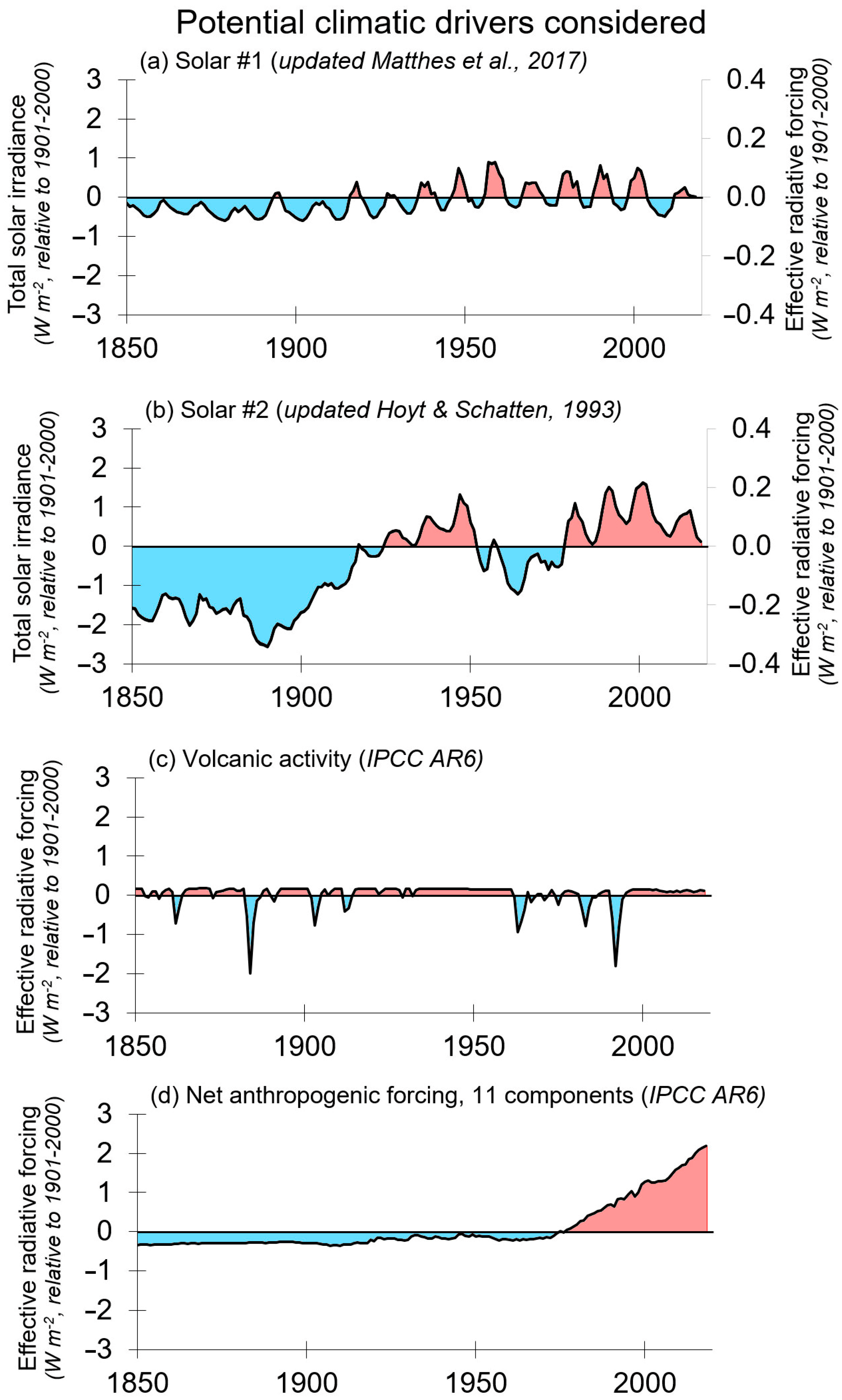
• Matthes et al. (2017) [11], the Total Solar Irradiance (TSI) dataset recommended by the CMIP6 organizers for estimating past solar activity, is a “low solar variability” estimate, just like the four datasets considered by the CMIP5 modeling groups for AR5 [3,7,12], and implies a much smaller role for the Sun than using a “high solar variability” dataset [7,12,13,14,15].

C2021 cautioned that both problems could significantly bias the attribution approach adopted by AR5 (and ultimately repeated by AR6 [1]) into prematurely concluding with unjustified confidence that the long-term global warming implied by the global temperature estimates was mostly human-caused [5]. Indeed, they showed that by altering the choice of TSI and/or the temperature records considered, they could explain the observed long-term warming as being anything from “mostly human-caused” to “mostly natural” or a mixture of both human-caused and natural factors.

1.1. Influence of C2021’s Findings on Recent Attribution Studies

Following the publication of AR6, the IPCC acknowledged that C2021 had not been considered by the AR6 authors since C2021 had missed the deadline for consideration by 10.5 weeks [16]. Therefore, the concerns raised by C2021 were apparently not considered for AR6’s attribution statement. Nonetheless, a number of recent global temperature attribution studies have explicitly considered different aspects of C2021 in their analysis [17,18,19,20,21,22].

Three of these studies agreed with C2021 that: (a) much of the long-term warming since the late 19th century could be explained in terms of changing solar activity and (b) the IPCC had substantially underestimated the solar contribution [17,18,22]. Two of the studies disagreed with C2021 and concluded that the solar contribution was very small [20,21]. The remaining study reached an intermediate conclusion, finding that TSI was the dominant climate driver up to 1960 but that afterward CO₂ appeared to dominate [19].

Each of these studies took a slightly different approach to attribution; had a different focus; and considered different aspects of C2021:

• Stefani (2021) [17] recognized the concerns about urban data raised by C2021 and based their analysis on global SST data instead. Acknowledging C2021’s point that it was unclear which (if any) of the many TSI datasets were correct, Stefani instead used the geomagnetic aa index as a proxy for solar activity citing previous work that found it to be useful as a solar proxy. Stefani then carried out a multilinear regression between SST, aa, and atmospheric CO₂ concentrations (i.e., the main component of IPCC’s “anthropogenic forcings”). The results suggested that solar activity explained between 30% and 70% of the observed long-term warming.
• Harde (2022) [18] used a two-layer energy balance model to evaluate the relative and absolute contributions of changes in (a) solar activity and (b) atmospheric CO₂ concentrations to Northern Hemisphere land and ocean temperatures since 1881. Considering C2021’s cautions about urbanization bias, Harde combined Soon et al. (2015)’s “mostly rural” land series [7] with Kennedy (2014)’s sea surface temperature record [23]. Harde carried out different “natural and anthropogenic” hindcasts for 6 of the 16 TSI records identified by C2021. The hindcasts using the TSI recommended to modelers for AR5 [3], i.e., Wang et al. (2015) [24], and AR6 [1], i.e., Matthes et al. (2017) [11], described the observed temperature changes very poorly. However, a striking fit was obtained (r = 0.95) between the hindcasted and observed temperatures when Scafetta et al. (2019)’s [12] update to Hoyt and Schatten (1993) [13] was used for TSI. This fit implied that 2/3 of the long-term warming for the Northern Hemisphere (oceans and rural land, 1881–2014) was solar in origin and only 30% was anthropogenic.
• Li et al. (2022) [19] used a statistical frequency analysis (using wavelet coherence) to evaluate the relative contributions of changes in TSI and CO₂ to global surface temperatures since 1880. Their chosen temperature record was Lenssen et al. (2019)’s global land and ocean series [25], which includes urban data. Therefore, Li et al. cautioned that their chosen temperature record was probably contaminated by non-climatic biases and referred the readers to C2021 for more details. They also cautioned that there was considerable debate over which TSI dataset to use, but that a choice was necessary and they decided on Coddington et al. (2016)’s TSI reconstruction [26]. As we will discuss later, this is very closely related to AR6’s Matthes et al. (2017) [11] series and was also one of C2021’s 16 TSI records. Li et al. found a very strong solar signal in the temperature changes up to about 1960, but afterward, the temperature changes shifted to being dominated by increasing CO₂. However, if they detrended the temperature record after 1960 to account for the presumed CO₂ warming, the very strong solar signal remained for the entire 1882–2020 period.
• Richardson and Benestad (2022) [20] reanalyzed some of the C2021 dataset using a multilinear regression in terms of TSI and anthropogenic forcings. However, they confined their analysis to C2021’s Northern Hemisphere “rural and urban” land series and dropped 2 of the 16 TSI records that ended before the 21st century. They were unable to find a substantial solar contribution to the long-term warming of the “rural and urban” series with any of the 14 remaining TSI records. They argued that the main difference between their reanalysis and C2021’s was that C2021 carried out a sequential regression rather than a simultaneous multilinear regression.
• Chatzistergos (2023) [21] did not use any TSI series for his analysis. Instead, he confined his analysis to a particular solar activity proxy—the solar cycle length (SCL). He noted that this proxy was one of the five solar proxies used in Hoyt and Schatten (1993)’s multiproxy TSI reconstruction [13]. This was one of the 16 TSI series identified by C2021—coincidentally the one identified by Harde (2022) as the best-fitting TSI record [18]. Comparing Hoyt and Schatten (1993)’s SCL component to several global land and ocean records (that incorporated urban data), he found that this individual proxy was unable to explain much of the post-1970 warming.
• Scafetta (2023)’s [22] attribution study used a 1-D energy balance model with a variable system response time to account for ocean buffering. The main temperature records considered were global land and ocean records. However, recognizing the concerns over urbanization bias in the land component, a secondary analysis only considered global sea surface temperatures.

The model considered three external forcing components—anthropogenic, volcanic, and solar. The first two factors were modeled using AR6’s recommended forcings series. However, for TSI, he generated three composite records based on different combinations of 8 of the 16 TSI series identified by C2021. Three of these TSI series were “low multidecadal variability” records and included AR6’s recommended series, i.e., Matthes et al. (2017) [11]. The other five showed “high multidecadal variability”, but he identified one of these records—Hoyt and Schatten (1993) [13]—as distinct from the other four.

Hence, he carried out hindcasts using four different averages of the multiple TSI records: (i) the average of all eight TSI records; (ii) the average of all TSI records except the three low variability records; (iii) the average of all TSI records except Hoyt and Schatten (1993) [13]; (iv) using only AR6’s recommended TSI. The hindcasts using only AR6’s recommended forcings were able to reproduce AR6’s attribution and led to the conclusion “that anthropogenic emissions account for substantially all of the observed global warming since the pre-industrial period (1850–1900) and that changes in solar activity are practically irrelevant”. However, the hindcasts using any of the TSI averages that included high multidecadal variability suggested a much greater solar role and nearly halved the apparent climate sensitivity to increasing CO₂. Furthermore, the hindcasts with the best fits to the observed temperatures were those that excluded the low multidecadal variability series from the TSI average, i.e., excluding those used for AR5 and AR6’s hindcasts.

1.2. IPCC AR6’s Positions on the Urbanization Bias and TSI Debates

AR6 has argued that the urbanization bias problem is small, i.e., <10% of the observed warming:

“No recent literature has emerged to alter the AR5 finding that it is unlikely that any uncorrected effects from urbanization […], or from changes in land use or land cover […], have raised global Land Surface Air Temperature (LSAT) trends by more than 10%, although larger signals have been identified in some specific regions, especially rapidly urbanizing areas such as eastern China [27,28,29]”

—AR6, Chapter 2, pp. 43–44 [1].

However, that AR6 claim contradicts several studies in the post-AR5 literature finding urbanization bias comprises more than 10% [7,9,10] of the estimated land warming. Indeed, ironically, one of AR6’s citations in the above quote—Shi et al. (2019) [29]—had specifically emphasized that recent literature had emerged questioning the AR5 finding. Surprisingly, Panmao Zhai, one of the co-chairs of AR6 had even drawn attention to the significance of Soon et al. (2015)’s [7] analysis of urbanization bias (and also their concerns about TSI) in his own work [30], yet these insights appear to have been overlooked by the authors of Chapter 2. According to a spokesperson for the IPCC (after consultation with Zhai), the reason for this particular oversight was apparently that “decisions on citations are up to the chapter team authors not the co-chairs” [16].

In terms of the debates over TSI choice, the CMIP5 project for AR5 had been criticized for only considering “low solar variability” TSI datasets and dismissing any “high solar variability” TSI datasets [7,12,13,15,31,32]. However, rather than expanding the range of TSI datasets considered, the CMIP6 organizers instead prioritized ensuring all participating models used “common CMIP6 forcings” for the hindcasts considered by AR6, e.g., see Section 1.5.4.3 and Cross-Chapter Box 1.4, Table 2 of AR6 [1]. Therefore, they only recommended one TSI dataset, i.e., Matthes et al. (2017)’s [11] “low solar variability” dataset.

1.3. Aims of This Study

In this article, we carry out a statistical attribution analysis of Northern Hemisphere land surface temperature time series using various combinations of natural and anthropogenic forcings. We propose that much of the conflicting conclusions reached by the recent climate change attribution studies described above [1,2,3,5,17,18,19,20,21,22] can be traced to differing choices on the two issues raised by C2021 [5], i.e.:

• How should the urbanization bias problem be accounted for?
• Which solar activity dataset(s) should be considered?

We note also that concerns about the reliability of both the CMIP5 and CMIP6 hindcasts in replicating observed climate changes have been expressed [31,33,34,35,36,37,38,39,40,41]. However, we suggest that most of the differences can be effectively distilled down to different views on these two specific issues.

C2021’s analysis had been based on a sequential two-step linear regression, but they had recommended future work should consider multilinear regressions [5]. This recommendation has since been echoed by others [20,22]. We adopt such a multilinear regression for this analysis.

To investigate the significance of the urbanization bias problem, we consider two different temperature records—both taken from C2021 [5]. The first record, “rural and urban stations”, uses all stations regardless of urbanization. This is equivalent to the temperature records considered by AR6. The alternative record is C2021’s “rural stations only” record.

To investigate the role of changing TSI datasets, we consider 2 of C2021’s 16 TSI datasets: (1) Matthes et al. (2017) [11] and (2) Scafetta et al. (2019)’s [12] update to Hoyt and Schatten (1993) [13]. The first is that considered by the CMIP6 modelers contributing to AR6, i.e., Matthes et al. (2017) [11].

The Matthes et al. (2017) TSI dataset is the arithmetic mean of another two of C2021’s compilations, i.e., (1) Naval Research Laboratory’s Total Solar Irradiance model version 2 (“NRLTSI2”) described in Coddington et al. (2016) [26] and (2) Max-Planck-Institut für Sonnensystemforschung’s Spectral And Total Irradiance Reconstructions model (“SATIRE”) described in Krivova et al. (2007; 2010) [42,43].

The NRLTSI2 model is a newer version of the NRLTSI1 model recommended to the CMIP5 modelers and described in Wang et al. (2005) [24] and other papers [44,45]. Both NRLTSI1 and NRLTSI2 relied on Hoyt and Schatten (1998)’s “Group Sunspot Number (GSN)” record [46] as the primary solar activity proxy. The SATIRE model also originally used this GSN as its primary solar activity proxy. However, the version used by Matthes et al. (2017) [11] replaced this with version 1 of the “International Sunspot Number (ISN)” [47] record. Kopp et al. (2016) calculated that changing the original GSN to ISN effectively flattens the long-term trend for both NRLTSI2 and SATIRE by increasing the implied sunspot numbers during the 18th and 19th centuries [48]. The various GSN/ISN reconstructions are the subject of considerable ongoing debate [49,50,51,52,53,54,55,56]. Nonetheless, because the NRLTSI2 and SATIRE models both use sunspot areas [57] as their main solar activity proxy for the period from 1874 onwards (with NRLTSI2 also using 10.7 cm radio flux readings [58] as an additional solar proxy from 1950 onwards), Kopp et al. (2016) noted that most of these changes were confined to the pre-1874 period [48]. The Matthes et al. (2017) reconstruction (and also our analysis in this article) avoids most of these issues by starting relatively close to this transition, i.e., in 1850.

The above TSI series comprised four of the “low solar variability” TSI estimates in C2021’s compilation [5]. However, for brevity, we only consider the Matthes et al. (2017) series since this was the one used for the CMIP6 hindcasts in AR6 [11].

Meanwhile, the alternative TSI dataset we consider is one of the “high solar variability” TSI estimates identified by C2021 [5], i.e., Scafetta et al. (2019)’s [12] update to Hoyt and Schatten (1993) [13]. This had already been identified before C2021 to be very well correlated with multiple climate records [7,13,32,59,60,61,62,63]. It also was singled out as one of the more noteworthy TSI records in C2021’s compilation [18,22]. Conversely, Chatzistergos (2023) [21] found that one of the five solar proxy records used by Hoyt and Schatten (1993) [13] was unable to explain recent warming trends on its own.

We then compare and contrast the results from each combination. Finally, we offer recommendations for further research into this challenging, but important, problem.

2. Methods and Datasets Used

2.1. Northern Hemisphere Land Air Temperature Series Used

Figure 1 compares the two different estimates of Northern Hemisphere land air temperatures considered in our analysis—a time series considering “rural and urban” stations and another considering “rural-only” stations. Both time series were downloaded from the Supplementary Materials for C2021 at https://doi.org/10.5281/zenodo.7088728 (accessed on 6 July 2023).

Both series are gridded mean temperature anomaly estimates calculated using temperature records from version 3 of the National Oceanic and Atmospheric Administration (NOAA)’s National Centers for Environmental Information (NCEI)’s Global Historical Climatology Network (GHCN) dataset [64]. Further details of the generation of these time series and a comparison with other estimates of Northern Hemisphere temperature time series are given by C2021 [5]. See also Figure S1 in the Supplementary Materials.

The “rural and urban” estimate of Figure 1a assumes that urbanization bias is a relatively minor problem. This would be consistent with AR6’s claim that urbanization bias represents less than 10% of the long-term warming in most estimates of land air temperature trends [1]. Therefore, all Northern Hemisphere stations in the GHCN dataset were used, regardless of their degree of urbanization. If AR6’s claim is correct, then this time series should be preferable to the “rural stations only” estimate of Figure 1c, since it is generated from a much larger sample of stations. This can be seen by comparing the station counts of both estimates in Figure 1b,d—noting that the vertical scales are different. Specifically, the “rural-only” estimate only uses 14% as many stations as the “rural and urban” estimate (a total of 586 stations vs. 4176 stations).

This philosophy of including all stations regardless of urbanization has dominated most attempts to estimate global temperature trends using weather stations. As a result, the “rural and urban” series is very similar to the equivalent time series by the Climate Research Unit (CRU) [65,66], Cowtan and Way (2014) [67], China Meteorological Administration (CMA) [68,69], Berkeley Earth [70], NASA Goddard Institute for Space Studies (GISS) [25,71]. and NOAA NCEI [64,72]—see Figure 2.

For this analysis, we use C2021’s “rural and urban” time series as representative of AR6’s position on the urbanization bias problem, i.e., that it is at worst a minor (<10%) concern—see AR6, Chapter 2, pp. 43–44. However, as can be seen from Figure 2, all of these estimates are very similar, i.e., all seven rural and urban records overlap almost exactly with each other. Therefore, the results from our analysis would be very similar if we used any of the other equivalent “rural and urban” estimates, e.g., the Northern Hemisphere land components of Refs. [25,64,65,66,67,68,69,70,71,72].

For C2021’s “rural stations only” estimate, four geographical regions in the Northern Hemisphere were identified that had most of the longest and most complete rural station records in the GHCN dataset. From these regions, only those stations which are currently rural in terms of both nightlight brightness and associated population were used. An exception was made for the earliest periods and some recent years for China since there was a shortage of fully rural data for China in these periods. Therefore, for China, some data from currently urbanized stations were used for parts of the record, but urbanization bias corrections were applied whenever this occurred.

Although C2021’s “rural stations only” estimate was derived from only four Northern Hemisphere regions, they noted that “the four regions alone account for more than 80% of the rural data for the early 20th century from either hemisphere”. They also carried out a detailed investigation into whether the “new rural-only estimate [is] better or worse than the standard estimates that include both urban and rural stations”—see Section 3.1.1 of C2021 [5].

Most of the current global/hemispheric temperature series were generated using temperature records that have been adjusted using an automated statistical homogenization technique such as the “Pairwise Homogenization Algorithm” (PHA) used by NOAA NCEI [64,72,73], rather than the original temperature records. The admirable goal of these automated homogenization processes is to attempt to statistically identify and correct for non-climatic biases that might be present in the raw temperature records [64,72,73]. However, C2021 [5] noted that such algorithms can inadvertently lead to “urban blending” whereby the urbanization biases of urban stations are partially “aliased” [74,75] into the homogenized records of rural neighbors [5,76,77]. This was recently confirmed by Katata et al. (2023) [78].

If we assume that the magnitude of the urbanization bias problem is as modest as AR6 proposes, then the urban blending problem of automated homogenization would also be relatively small—indeed this has been argued by Hausfather et al. (2013) [79]. Therefore, the rural and urban time series was generated from the widely used PHA-adjusted GHCN dataset. However, since the purpose of developing a “rural-only” series is to reconsider this assumption, C2021 recognized that using the PHA-adjusted GHCN dataset for evaluating rural temperature trends would be erroneous [5]. Hence, the rural-only time series was generated from the original non-PHA-homogenized GHCN dataset.

Therefore, to develop the rural-only time series, different approaches to correcting for non-climatic biases needed to be applied. The first step was to remove urbanization bias by excluding all non-rural stations for three of the regions (Arctic, USA, and Ireland) and applying empirically derived urbanization bias adjustments to any of the partially urbanized Chinese stations used for increasing the spatial and temporal representativeness of the region [5,7,37,76]. Documented time-of-observation biases (TOB) associated with the USA network were accounted for using NOAA NCEI’s empirically based TOB adjustments [80,81]. Additional biases due to the documented degradation in station exposure of many USA stations [82] were corrected by means of a regionally averaged and empirically derived bias correction [5,7]. Finally, biases due to documented station moves associated with the longest rural Irish station in the dataset were identified and corrected for experimentally in consultation with the station owners [7].

Doubtless, these adjustments have not yet identified all of the non-climatic biases that might be present in the temperature data. Some of us are continuing research into collating more station metadata to identify further potential non-climatic biases in the GHCN datasets, e.g., [76,77,83]. Nonetheless, these manual homogenization adjustments based on station information have the advantage of avoiding the urban blending problem unlike the standard automated statistical homogenization adjustments currently used by most groups.

O’Neill et al. (2022) [83] have recently described additional concerns over the PHA-adjusted GHCN dataset in a detailed assessment of more than 800 European GHCN stations. They found that less than 20% of the homogenization adjustments applied to a given day’s version of the GHCN dataset are consistently applied. Also, they found that less than 20% of the adjustments could be clearly associated with known station changes documented in available station metadata.

In this study, we proceed with the two temperature series described above and shown in Figure 1. A visual comparison of the two series shows that while there are clear similarities between the “rural and urban” and “rural-only” estimates, there are also several key differences:

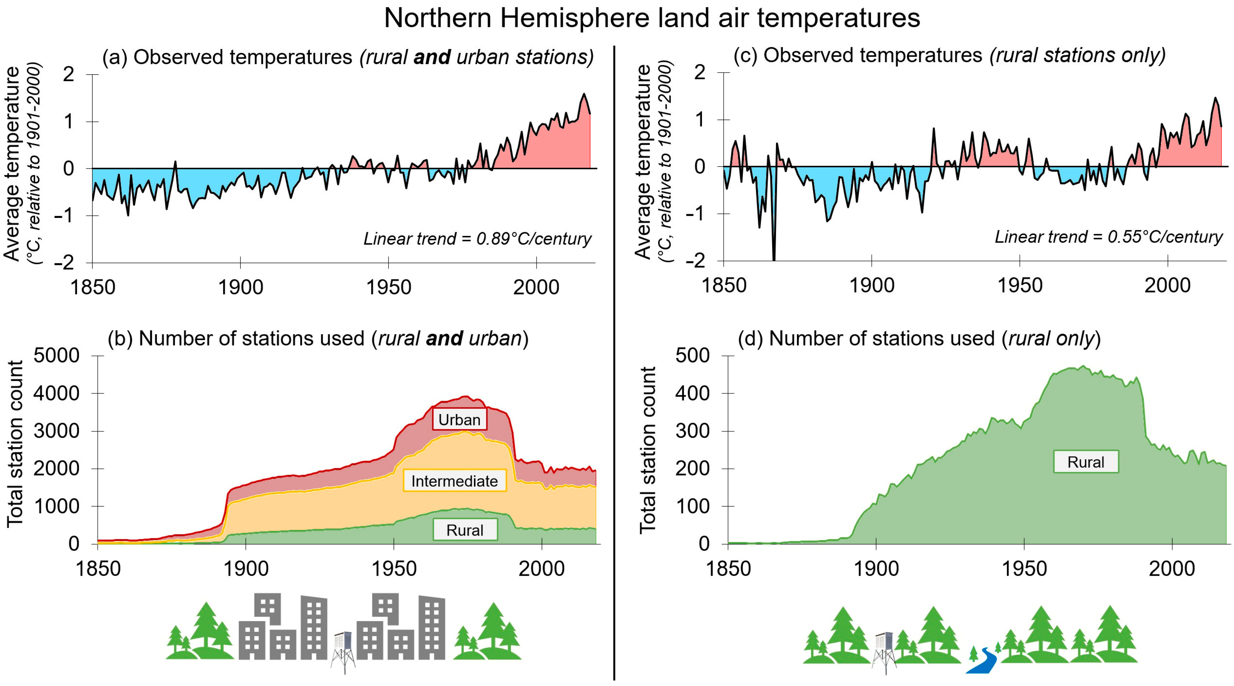
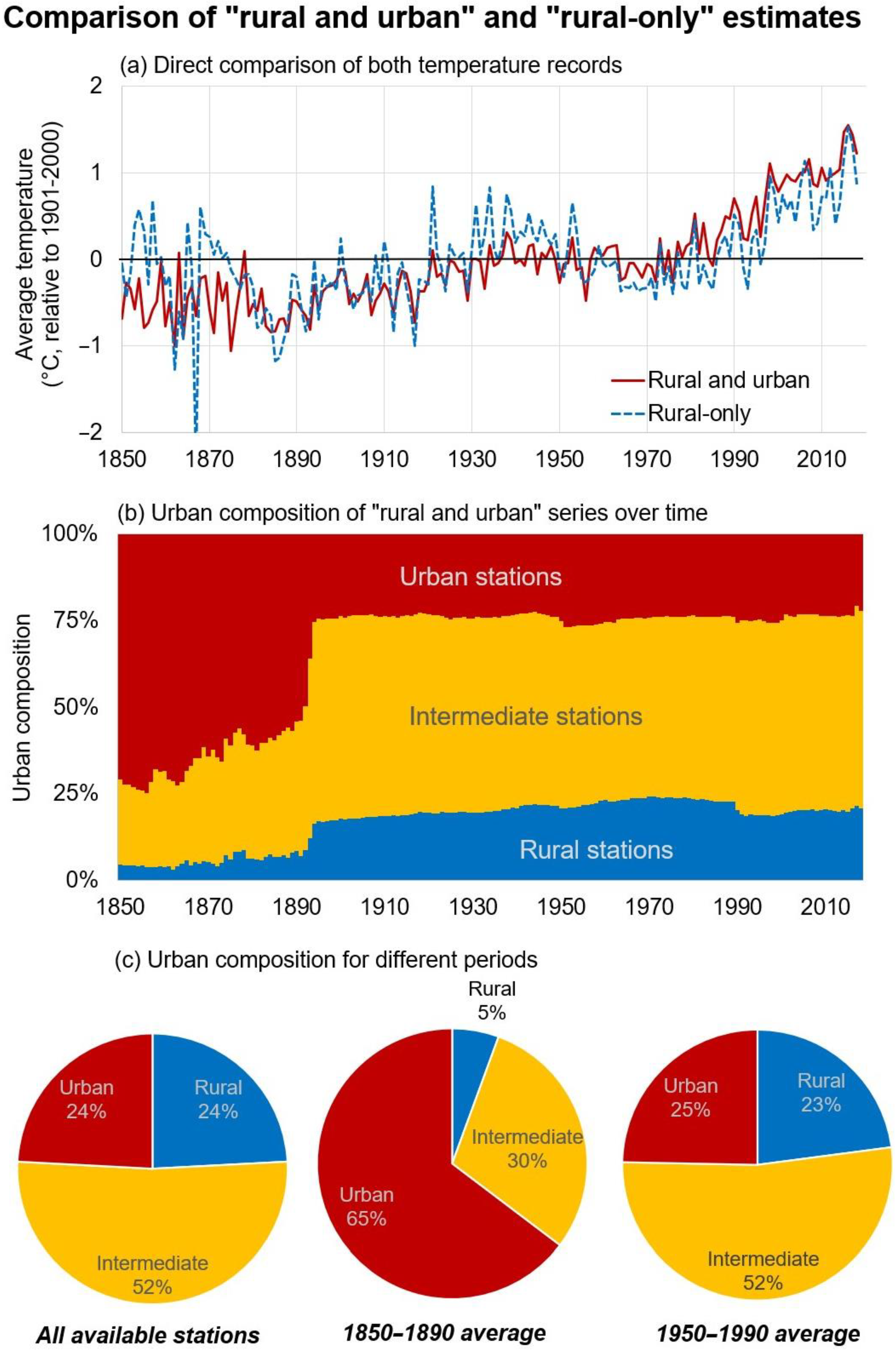
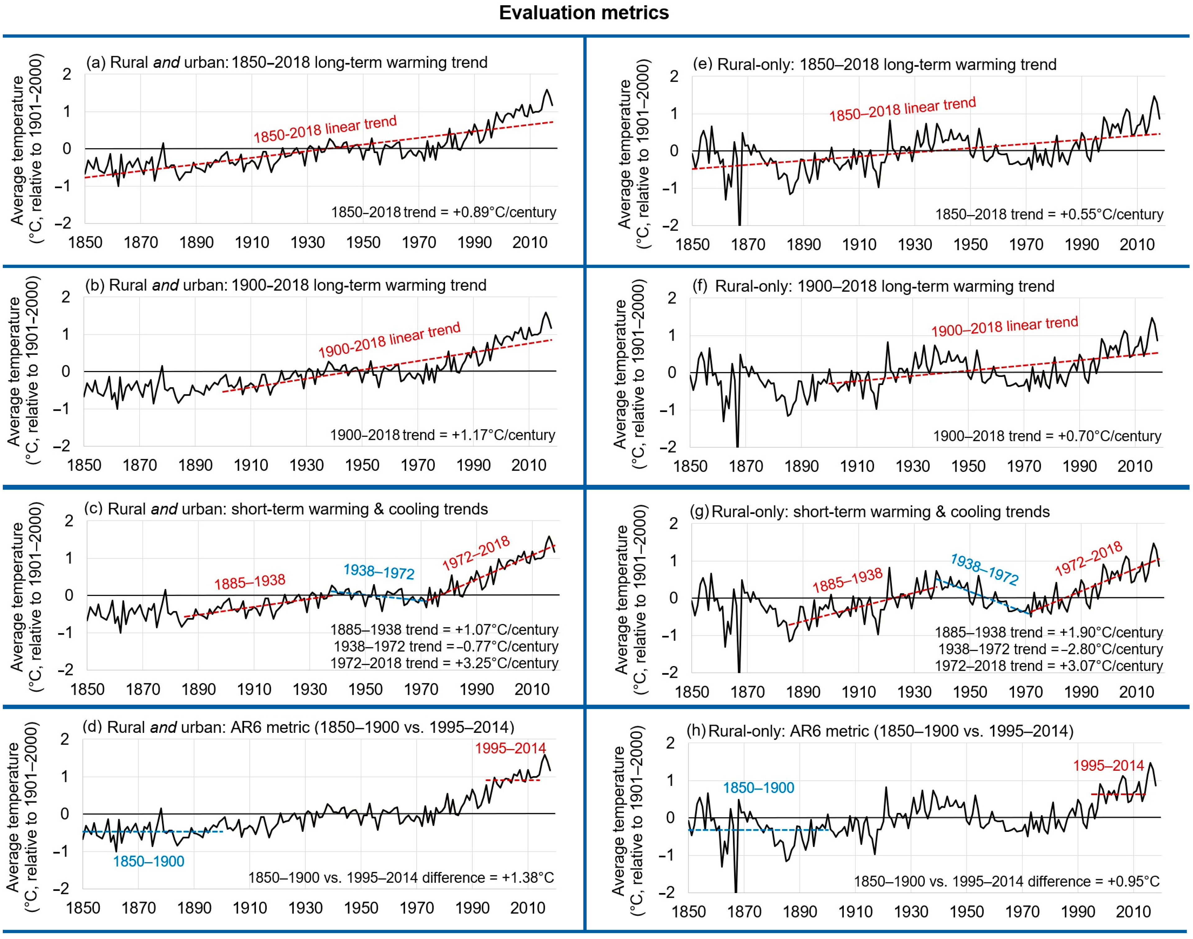
• The “rural-only” estimate is noticeably “noisier”, i.e., the magnitudes of the fluctuations from year to year are larger. This is largely a consequence of the reduced number of stations, as discussed in C2021. However, it is noteworthy that the timing of the multidecadal warming and cooling periods for both series are qualitatively similar.
• The long-term (1850–2018) linear warming trend of the “rural and urban” series is 62% higher than that for the “rural-only” series, i.e., +0.89 °C/century compared to +0.55 °C/century. C2021 argue that much of this extra warming in the “rural and urban” series is due to a combination of urbanization bias and “urban blending” arising from the homogenization process.
• While the “rural and urban” series implies an almost continuous long-term warming, the “rural-only” series suggests a much more nonlinear behavior. That is, the “rural-only” series suggests that temperatures have alternated between multidecadal periods of cooling and periods of warming since at least the mid-19th century.

The nonlinear nature of the “rural-only” series has implications for our analysis since we will be predominantly focusing on linear trends and linear regressions. With regards to the relatively warm 1930s–1940s period suggested by the rural-only series, we note it has similarities to the early-20th-century warm period that has been noted for the Arctic region [37,84,85]. We also note there seems to have been a slight mid-19th-century warm period that is not apparent from the “rural and urban” estimates. However, we caution that the number of stations available for the 19th century is especially limited for the rural-only series, as can be seen from Figure 1d.

Some might argue that the fact that the following all imply a warming trend over their entire records indicates that the long-term warming trends implied by the various land station-based series shown in Figure 2 are also reliable [86]:

(a)

Ocean heat content measurements (1955-present) [87,88];

(b)

Weather-balloon-based estimates of lower- and mid-troposphere air temperatures (1958-present) [89];

(c)

Satellite-based estimates (1978-present) [89,90,91];

(d)

Satellite-based estimates of “surface skin temperatures” (2003-present) [86].

However, we note from Figure 1c that the “rural-only” estimate also suggests warming trends over all these periods. Therefore, merely providing evidence of “global warming” over these relatively short periods is inadequate for resolving which of the two series is more reliable.

Given these concerns over the extent of urbanization biases in the land surface temperature (LST) records, one might consider bypassing the urbanization bias problem by using sea surface temperature (SST) data instead. This was the approach taken by Stefani (2021) [17] and the use of SST data was also part of the analyses of Harde (2022) [18] and Scafetta (2023) [22]. Indeed, C2021 also noted that their “rural-only” estimate was qualitatively similar to Northern Hemisphere sea surface temperature (SST) estimates as well as several Northern Hemisphere temperature proxy-based estimates.

We agree that the SST data should be unaffected by urbanization biases—unless the SST data has been adjusted to better match the LST data as some groups have done, e.g., Cowtan et al. (2018) [92]. However, we caution that the SST data also have their own non-climatic bias problems—especially before the 1950s. Hence, Jones (2016) has argued that the LST component of global and hemispheric temperature estimates is more reliable than the SST component [93].

For a detailed discussion of the uncertainties associated with the non-climatic biases of SST data, see Section 3.3 of C2021 [5] or Kent and Kennedy (2021) [94]. However, one of the key challenges is the fact that the available SST data is very sparse before the 1950s (especially for the Southern Hemisphere) [95]. Other challenges are the changes in instrumentation and measurement practices over time. It is known that different SST measurement practices can imply different multidecadal trends. For instance, Davis et al. (2019) found that SST measurements taken via “engine-room intake” implied a substantial global cooling trend from 1950 to 1975, while those taken by “bucket” measurements implied a slight warming over the same period [96]. C2021 noted that the former would be consistent with the “rural-only” LST series while the latter would match better with the “rural and urban” LST series [5].

Therefore, for the current study, we will limit our analysis to the two LST records. However, we encourage further research into resolving the uncertainties associated with the SST data [94] and we recognize that studies using SST instead of urbanized LST have at least bypassed the urbanization bias problem [17,18,22].

In Figure 3, we highlight an additional challenge in assessing the extent of urbanization bias in the “rural and urban” series—the relative urban/intermediate/rural composition of the series varies substantially over the period of the record. As can also be seen from Figure 1b, in the earlier parts of the record the fraction of available stations that remain rural today is very small—especially for the mid-to-late 19th century. For example, only 5% of the available stations for the 1850–1890 period remain rural today, while 65% are now fully urban—see Figure 3c.

Initially, one might think that this 19th-century urban composition is not so serious since the relative magnitude of the urban heat islands associated with those stations would have been much smaller than now (in the early 21st century). However, it is important to remember that the urbanization bias problem largely arises from long-term gradual warming biases. The majority of the stations used for comparing the mid-19th century to the present are now urbanized. Counterintuitively, for more recent decades, even though the rate of urbanization has accelerated, the urbanization bias is in some ways less of a problem for the modern period—since there is a much larger number of rural stations available.

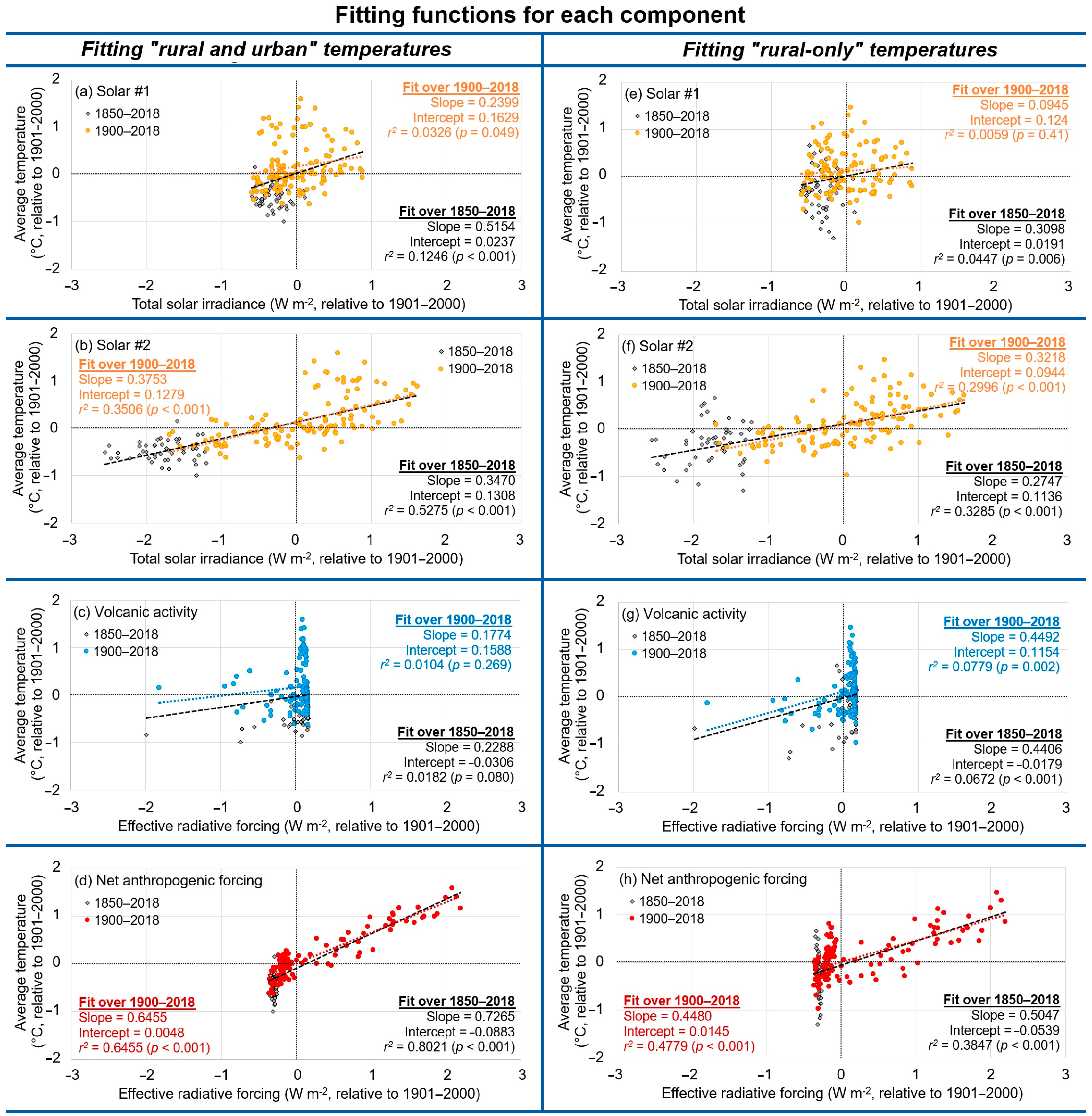
2.2. Potential Climatic Drivers Used by Each Approach

The CMIP6 hindcasts that formed the main basis for AR6’s attribution statement considered two natural forcings (solar and volcanic) and multiple anthropogenic forcings (chiefly, increasing greenhouse gases and aerosols, but with some other contributions). However, while the CMIP6 contributors were all strongly recommended to use the Matthes et al. (2017) [11] solar activity dataset, C2021 identified a wide range of plausible solar activity datasets that were also in the literature. Therefore, to assess the sensitivity of the results to changes in the solar activity series used, we consider two different solar activity datasets. We downloaded both of these from the Supplementary Materials of C2021 at https://doi.org/10.5281/zenodo.7088728 (accessed 6 July 2023).

“Solar #1” is the one recommended to the CMIP6 contributors, i.e., Matthes et al. (2017) [11], although it has been updated to 2018 by C2021. “Solar #2” is Scafetta et al. (2019)’s [12] update of the Hoyt and Schatten (1993) [13] time series to 2018. The time series are plotted in units of W m⁻² relative to their 1901–2000 average in Figure 4a,b, respectively. We have also included a secondary y-axis on these two figures showing the equivalent values in terms of the effective radiative forcing (ERF) calculated following AR6’s recommendation in Section 7.3.4.4 of AR6 [1]. This involves scaling TSI by ×0.1278.

As can be confirmed visually by comparing Figure 4a,b, these two different TSI estimates offer a strikingly different history of changes in solar activity since 1850. We encourage readers to study C2021 for a detailed discussion of why such differences still exist today. However, in essence, the key differences relate to different philosophies on two issues: (a) the choices of solar proxies used for the pre-satellite era and (b) the satellite TSI composite used for calibration.

In terms of satellite TSI composites, there are several available, but the most distinct composites are:

• The Active Cavity Radiometer Irradiance Monitor (ACRIM) composite [12,32]. This implies TSI increased between solar minima during the 1980s and 1990s but decreased during the early 21st century.
• The Physikalisch-Meteorologisches Observatorium Davos (PMOD) composite [97,98]. This implies TSI has slightly decreased between solar minima over the entire satellite era, i.e., 1979-present.
• The Royal Meteorological Institute of Belgium (RMIB) composite [99,100]. This implies TSI has remained remarkably constant between solar minima over the entire satellite era.

The choice of satellite composite used for calibration has considerable implications for the most suitable solar proxies to use for the pre-satellite era, i.e., before 1979. If the RMIB composite is correct, then it could be argued that TSI largely follows the sunspot cycles and simply calibrating a suitable sunspot number record should give a reasonable TSI reconstruction for the pre-satellite era, e.g., Dewitte et al. (2022) [100]. If the PMOD composite is correct, then a suitably rescaled sunspot number record should also give a reasonable TSI reconstruction, but the addition of extra solar proxies could potentially improve accuracy, e.g., Wang and Lean (2021) [101]. The Matthes et al. (2017) [11] reconstruction used by CMIP6 for AR6 appears to have taken this second philosophy.

However, if the ACRIM composite is correct, then reconstructing TSI for the pre-satellite era becomes a much more challenging problem. That is because the variability in the TSI of solar minima implied by ACRIM is not captured by the sunspot number record (which reaches a minimum of exactly zero sunspots every solar minimum). ACRIM therefore implies that long-term (inter-cycle) trends in TSI need to be considered as well as the short-term (~11-year solar cycle) variability. Hoyt and Schatten (1993) [13] was a very significant TSI reconstruction specifically because it used multiple solar proxies to attempt to capture both the short-term (~11-year solar cycle) and the long-term (inter-cycle) multidecadal variability—see also Hoyt (1979) [102]. Scafetta et al. (2019) [12] updated this 1993 reconstruction to 2018 using the ACRIM team’s composite.

We encourage interested readers to repeat our analysis using other combinations of the 20 TSI time series in the Supplementary Materials of C2021 or indeed any other available TSI time series of interest. In principle, our analysis could also be repeated using annually resolved solar activity proxies other than TSI, e.g., geomagnetic activity indices [17].

For volcanic and anthropogenic components, we use the relevant time series from the IPCC AR6 WG1 Annex III dataset [103], which we downloaded from https://doi.org/10.5281/zenodo.5705390 (last accessed on 6 July 2023). We rescaled these time series relative to their 1901–2000 average. Both time series are plotted as effective radiative forcing in units of W m⁻² relative to the 1901–2000 average in Figure 4c,d.

To simplify our analysis, we use the single “all anthropogenic forcings combined” time series provided by the IPCC Annex III dataset. We note, though, that this time series actually comprises 11 individual components.

According to the framework used by AR6, once a “forcing” time series has been converted into an effective radiative forcing (ERF) time series (in W m⁻²) by the application of suitable theoretical and/or semi-empirical calculations, they are almost directly comparable. Hence, many studies will routinely sum these time series together. Therefore, for brevity, we follow that approach for evaluating the anthropogenic contribution. However, for the statistical analysis in this paper, each component of the “net anthropogenic forcings” could in principle be evaluated separately. We have not done so here, but for reference, we have plotted all 11 components in the Supplementary Materials—see Figure S2.

Before we discuss our statistical analysis approaches, it might be useful to briefly compare and contrast our four potential fitting parameters in Figure 4. Comparing Solar #1 and Solar #2 in Figure 4a,b, we can see that both reconstructions are consistently below the 20th-century average for the 2nd half of the 19th century and both show short-term rises and falls over the ~11-year solar cycle. However, Solar #2 suggests a far more dynamic history for TSI variability with the ~11-year periodicity superimposed over multidecadal trends that are often greater in magnitude than the rises and falls associated with the ~11-year cycle. The changes from the other “natural forcing”, i.e., volcanic activity, are much shorter in duration and episodic in nature. As can be seen from Figure 4c, the changes associated with a given volcanic event only last for 2–3 years. Finally, the net anthropogenic forcing series is almost flat for most of the study period but starts to steadily increase dramatically during the 1970s. Interested readers might note from Figure S2 that this shape of the “net anthropogenic forcings” is subtly different from the calculated “CO₂ forcing” that is more monotonic in nature—due to the other 10 components, chiefly the two aerosol components.

Figure 4. Time series of the four forcings considered in this analysis. (a,b) represent two different estimates of solar variability since the mid-19th century; (c) plots the volcanic forcing; (d) plots the combined anthropogenic forcings. For more details on the two solar activity series, see Connolly et al. (2021) [5]. The volcanic activity and anthropogenic forcing time series are taken from the IPCC AR6 WG1 Annex III dataset [103].

Figure 4. Time series of the four forcings considered in this analysis. (a,b) represent two different estimates of solar variability since the mid-19th century; (c) plots the volcanic forcing; (d) plots the combined anthropogenic forcings. For more details on the two solar activity series, see Connolly et al. (2021) [5]. The volcanic activity and anthropogenic forcing time series are taken from the IPCC AR6 WG1 Annex III dataset [103].

2.3. Statistical Analysis Used

We take two separate approaches to fitting our target temperature records. The first approach is to carry out an OLS linear regression between each of the four radiative forcings time series (Figure 4) and either the “rural and urban” or the “rural-only” time series (Figure 1). We refer to this approach as individual component fitting. This allows us to identify an upper bound for how much of the linear trends of each temperature series could potentially be explained in terms of each individual component, i.e., the maximum potential contribution.

For our main analysis, we will carry out the regression over the entire 1850–2018 record. However, as can be seen from Figure 1, the number of stations available for the mid-to-late-19th century is small—especially for the “rural-only” series. Moreover, from Figure 3b,c, it can be seen that the “rural and urban” series is dominated by urban stations for this period. Therefore, as a secondary analysis, we will repeat our regression fittings using the shorter 1900–2018 period. The “rural-only” series uses at least 100 stations throughout this period and it has been estimated that global temperature trends can be reliably estimated with as few as 50 well-spaced locations [104,105] at the annual timescale our analysis considers. Meanwhile, the percentage of rural stations in the “rural and urban” series increases from 4% in the 1850–1890 period to ~20–24% throughout the 1900–2018 period.

The second approach is a multiple linear regression using a combination of two or three of our components. This regression is also OLS. As for our individual component fittings, our main analysis is carried out over the entire 1850–2018 period. However, again as a secondary analysis, we will repeat our regression fittings using the shorter 1900–2018 period. For each temperature series, we consider four combinations:

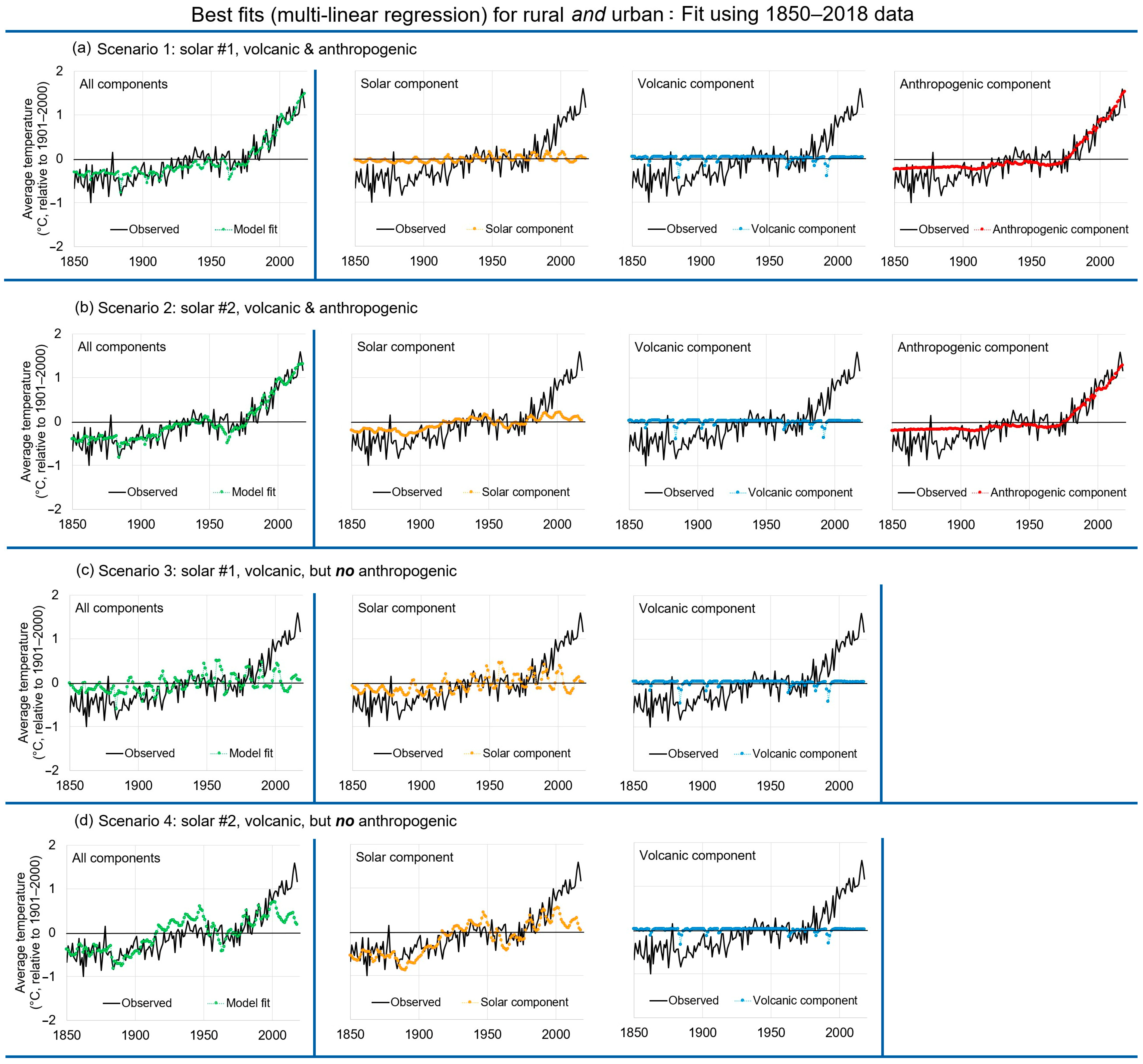
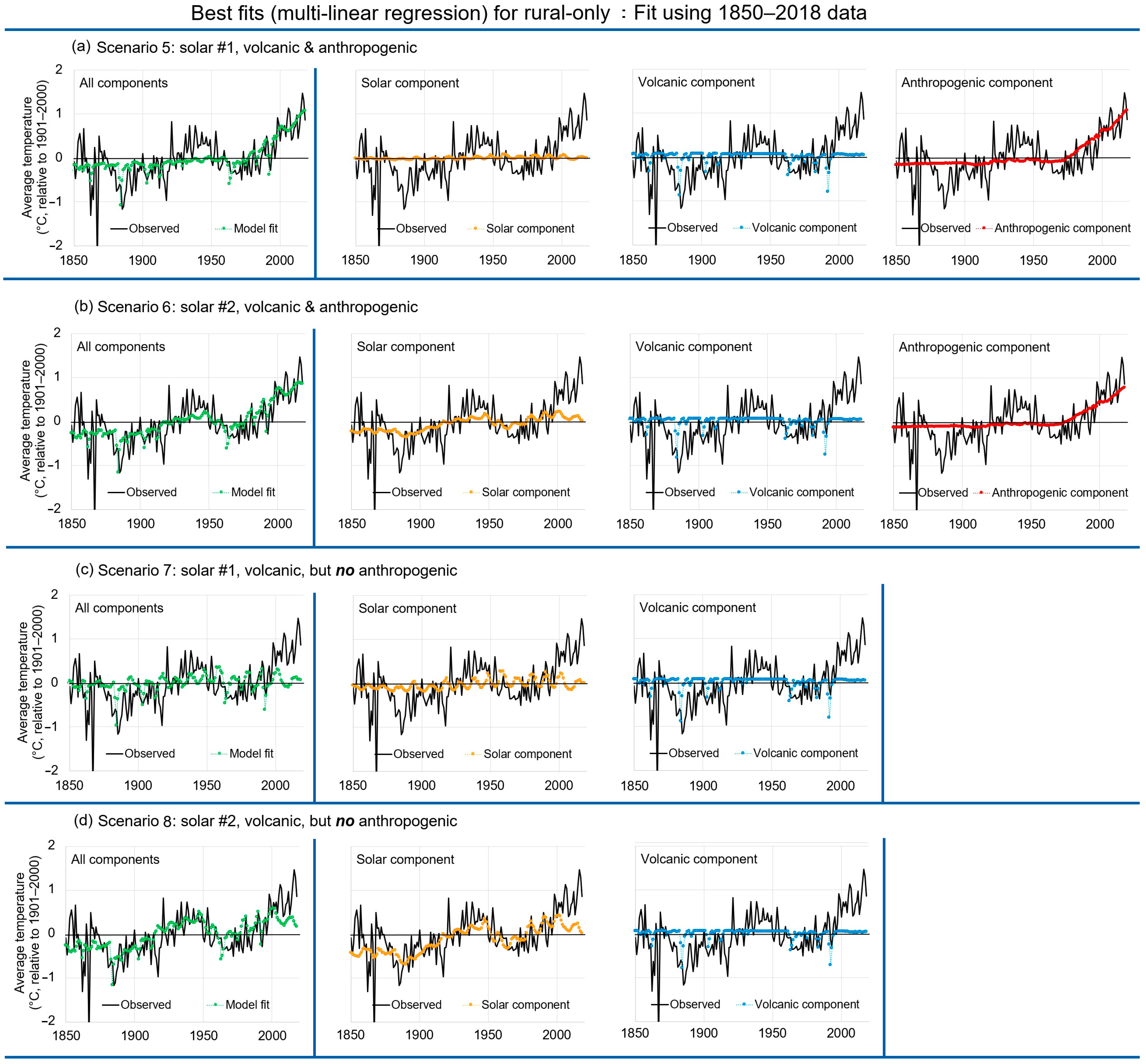
• Natural and anthropogenic (CMIP6): Solar #1, volcanic and anthropogenic components, i.e., equivalent to that adopted for the “natural and anthropogenic forcings” CMIP6 hindcasts;
• Natural and anthropogenic (alternative): Solar #2, volcanic and anthropogenic components, i.e., the same as for the CMIP6 hindcasts, except using the other solar activity dataset;
• Natural only (CMIP6): Solar #1 and volcanic, i.e., equivalent to the “natural forcings only” CMIP6 hindcasts;
• Natural only (alternative): Solar #2 and volcanic, i.e., an alternative “natural forcings only” scenario.

There clearly are many different methodologies that could be used for this type of analysis [1,2,3,5,7,13,17,18,20,22,106,107,108,109,110,111,112,113].

We emphasize that the relatively simple statistical approach adopted in this paper appears to reproduce reasonably well the findings of the more complex GCM-based attribution of AR6 [1] and Gillett et al. (2021) [2] provided it is carried out with the equivalent time series to those used by Gillett et al. (2021) [2].

Nonetheless, given that the results of our analysis only replicate AR6’s attribution statement when it is applied using AR6’s choices with regard to the TSI and urbanization bias debates, it is probably worth directly comparing and contrasting our approach to the attribution analysis that AR6 used, i.e., Gillett et al. (2021) [2].

Arguably, the biggest methodological difference between the two approaches is that our statistical fitting approach fits the time series for each component directly to the temperature records, whereas Gillett et al. (2021) [2] fits various climate model hindcasts to the temperature records. These hindcasts were themselves generated using the relevant natural and anthropogenic component time series as model inputs (often summarized in terms of radiative forcing units for comparison). Hence, both approaches use similar inputs, but Gillett et al. (2021)’s [2] approach uses climate models as an additional intermediate step.

Recently, Scafetta (2023) has suggested a regression methodology where the climate was allowed to respond to solar forcing differently than to the other radiative forcings. He suggested that the way changes in solar activity are modeled by current GCMs may be underestimating the climatic response to changing TSI by a factor of between 4 and 7. This is because the models do not allow for the possibility that the climate response to total solar activity changes might be greater than that predicted based on ERF calculations [22]. This is consistent with Chylek et al. (2020)’s findings [111]. Our statistical multilinear regression approach should also mitigate this potential problem. Harde (2022)’s two-layer model also appears to have reduced this problem by allowing for the possibility of solar-induced climate feedbacks [18].

There are several other technical differences between our approach and that of Gillett et al. (2021) [2]:

• Gillett et al. (2021) [2] applied total least squares (TLS) linear regressions instead of OLS. Both forms of linear regression generally yield similar results. However, OLS assumes that the x-axis (in this case, year) is well determined. Because Gillett et al. (2021) [2] attempted to fit climate model hindcasts, they argue that TLS is preferable since this allows for the fact that, due to the internal variability of climate models, there can be some uncertainty in the timing of temperature changes.
• Gillett et al. (2021) [2] fitted global land and ocean temperatures, whereas our analysis fits the Northern Hemisphere land-only temperatures.
• Gillett et al. (2021) [2] did not consider the possibility of urbanization bias contamination or study the effects of varying the choice of the TSI dataset.

Finally, we note that for the two solar activity time series, we use the original TSI values instead of the calculated ERF values, i.e., the primary y-axes of Figure 4a,b instead of the secondary y-axes, since the ERF values are derived from the TSI time series (via a linear scaling). However, the results are identical (not shown) when we use the ERF values. This is because OLS identifies the best linear relationship between the explanatory series and the target series that minimizes the squares of the residuals. Scaling the input time series by a linear (non-zero) constant only changes the values of the slope and intercept of this linear fitting, but not the goodness of the fit or the final results.

2.4. Evaluation Metrics Used

A challenge for a climate change attribution study such as this one or AR6’s equivalent analysis is to decide on the most suitable metrics for comparing the fitted contributions to the observed climate change—in this case, Northern Hemisphere LSAT.

We consider four sets of metrics for evaluating the fits. We illustrate these in Figure 5, demonstrating how they are applied to the two target temperature records:

• For our main analysis, we will use a fairly straightforward metric—the long-term linear trend over the length of the data records, i.e., 1850–2018. As we shall see, this is usually a warming trend and reflects the long-term hemispheric warming since the start of the record (1850). Comparing Figure 5a,e, we note that the rural and urban trend is 60% higher than that for the rural-only record. It seems plausible that at least some of this extra warming is a result of urbanization bias.
• Meanwhile, as discussed in Section 2.3, the number of stations used for the 19th century is particularly low and mostly limited to stations that are now urbanized. For these reasons, we repeat our analysis by fitting over the shorter 1900–2018 period. Similarly, our second evaluation metric is the 1900–2018 linear trend. We can see from Figure 5a–d that these trends are higher for both the rural and urban series and the rural-only series. However, comparing Figure 5b,f, we note that the rural and urban trend is still substantially higher (67%) than that for the rural-only record.
• Still, using a single long-term linear trend is a somewhat crude metric since the LSAT trends are quite nonlinear—especially for the rural-only series—and neither are the trends for any of the three factors (see Figure 4). Therefore, for our third set of metrics, we consider multiple shorter-term linear trends. As can be seen from Figure 5c,g, both temperature series imply an alternation between warming and cooling periods over the course of the records. Therefore, we calculate the linear trends over three periods, corresponding to local minima and maxima common to both temperature series, i.e., warming from 1885–1938; cooling from 1938–1972; warming from 1972–2018. We note that the differences between the rural-only and rural and urban series are actually greatest for the early-20th-century warming and mid-20th-century cooling rather than the more recent warming period. This might be counterintuitive since urbanization has accelerated in recent decades. However, as discussed in Section 2.1, the urbanization bias problem is complicated by the fact that the availability of rural stations has also increased substantially over recent decades—see Figure 3.
• Our fourth metric completely avoids the use of linear trends and instead involves a comparison of the temperature averages over two fixed time periods. Specifically, we use the difference between the 1850–1900 average and the 1995–2014 average for comparison with several discussions in both AR5 and AR6, e.g., Section 7.3.5.3 (“Temperature Contribution of Forcing Agents”) of AR6 [1]. We refer to this metric as the “AR6 comparison metric”. In terms of this metric, the rural and urban series is 45% higher than the rural-only series—see Figure 5d,h.

We therefore will consider all four sets of metrics for our attribution. However, we note that further work could consider other metrics. For example, Lüning and Vahrenholt (2017) [114] argue that the use of 1850–1900 as a baseline for evaluating long-term warming is inappropriate from a paleoclimatic context since it incorporates the end of the Little Ice Age. Instead, they suggest 1940–1970 as a more suitable baseline. Meanwhile, Scafetta (2021a) [10] used the differences between the decadal averages of 1945–1954 and 2005–2014.

3. Results and Discussion

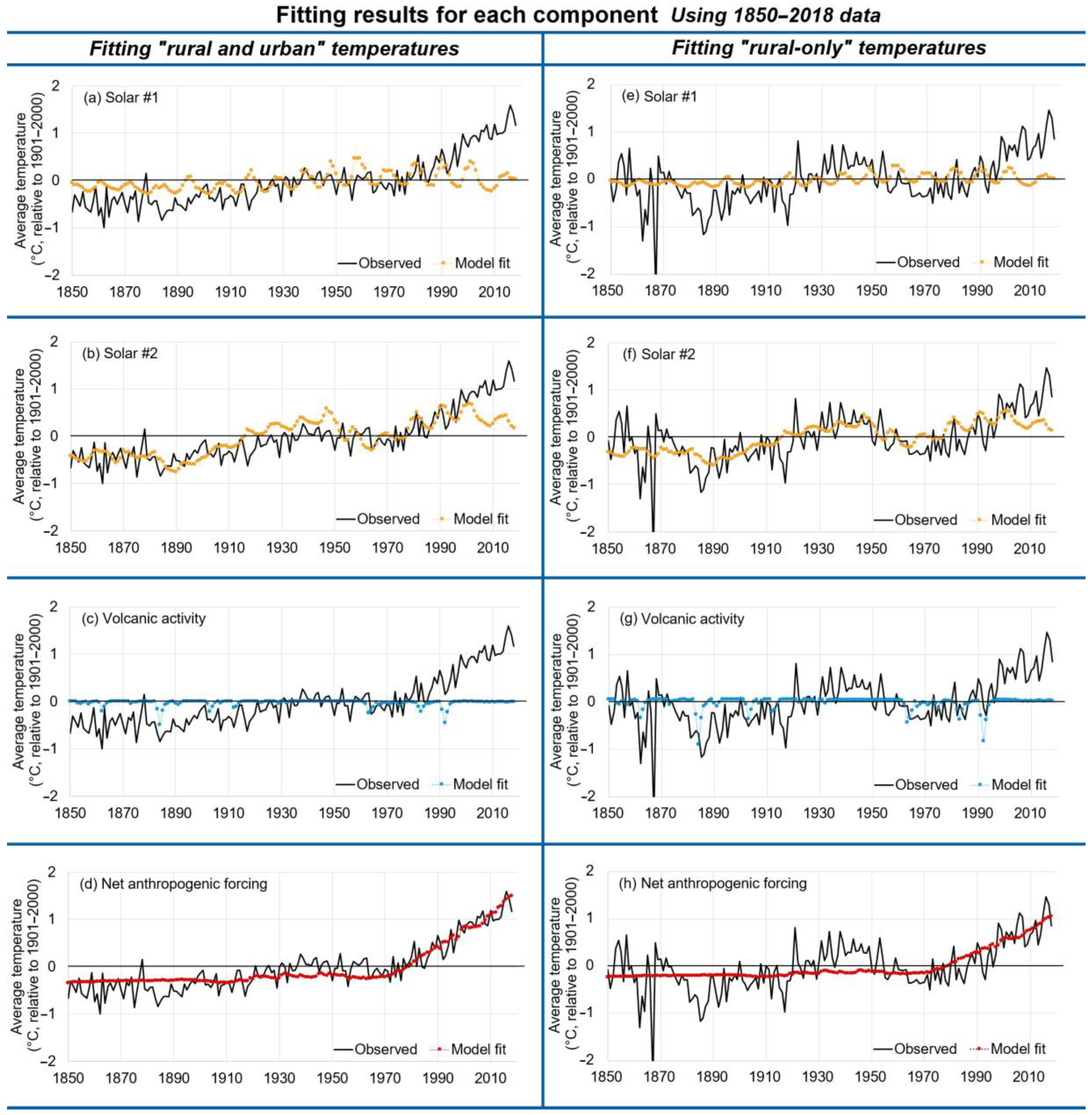
3.1. Results from the Individual Component Analyses

Figure 6 shows the OLS linear relationships between each of the components and the two temperature records using either the full 1850–2018 period or the shorter 1900–2018 period. We note that for both temperature records, the anthropogenic forcing has the highest r² value. However, as we saw from Figure 4d, the anthropogenic forcing series is relatively flat for most of the record until the 1970s. Therefore, most of the data points up until this period are clumped in a small region in Figure 6d,h. In contrast, the points are more evenly spread over the entire record for the Solar #2 fits. This suggests a more consistent influence from TSI than anthropogenic forcings over the entire record.

The statistics associated with the Solar #1 fits are much weaker than that for Solar #2. Indeed, using the shorter 1900–2018 period for fitting, the linear relationship is not statistically significant for the rural-only record (p > 0.05) and barely statistically significant for the rural and urban record (p = 0.049). The fits for volcanic activity are quite weak, and they are not statistically significant for the rural and urban records either (p > 0.05). Nonetheless, let us now consider the results when we apply these linear relationships to each component.

Figure 7 shows the results from the first stage of our analysis, i.e., the individual component analysis, using the full 1850–2018 record. The corresponding evaluation metrics are provided in

Table 1. Results of individual component analysis fitting of the “rural and urban” temperature record over the 1850–2018 period in terms of the various evaluation metrics.

Evaluation Metric	Rural and Urban	Solar #1	Solar #2	Volcanic	Anthropogenic
Trend-based	Trend (°C/century)	%	%	%	%
1850–2018	0.89	21%	70%	0%	82%
1900–2018	1.17	15%	39%	−2%	107%
1885–1938	1.07	28%	201%	8%	21%
1938–1972	−0.77	−32%	222%	35%	18%
1972–2018	3.25	−7%	18%	4%	109%
Period-based	Difference (°C)
AR6	1.37	12%	66%	2%	88%

and

Table 2. Results of individual component analysis fitting of the “rural-only” temperature record over the 1850–2018 period in terms of the various evaluation metrics.

Evaluation Metric	Rural-Only	Solar #1	Solar #2	Volcanic	Anthropogenic
Trend-based	Trend (°C/century)	%	%	%	%
1850–2018	0.55	20%	89%	−2%	93%
1900–2018	0.70	16%	53%	−6%	124%
1885–1938	1.90	9%	89%	9%	8%
1938–1972	−2.80	−5%	49%	19%	3%
1972–2018	3.07	−4%	15%	8%	80%
Period-based	Difference (°C)
AR6	0.95	9%	75%	4%	87%

. The equivalent results using the shorter 1900–2018 period are provided in the Supplementary Materials as Figure S3 and Tables S1 and S2. The fitting coefficients and statistics for all fits are provided in the Supplementary Materials Excel file.

We can already understand AR6’s attribution statement from this individual components analysis. If we use “Solar #1”, then the maximum warming (upper bound) we can explain in terms of the two natural climatic drivers is 0.19 °C/century (21% of the observed 1850–2018 warming trend). It can only explain up to 12% of the AR6 comparison metric.

The other natural factor considered, i.e., the volcanic contribution can only contribute a slight cooling (or a slight relative warming of ~2% in terms of the AR6 comparison metric). Therefore, this already implies that the long-term warming is mostly human-caused, i.e., AR6’s conclusion.

Meanwhile, the anthropogenic forcings can explain almost all the observed 1850–2018 warming trend (0.73 °C/century, i.e., 82%) and 88% of the AR6 comparison metric—Table 1. It even slightly overestimates the 1900–2018 trend with 107% of the observed warming. It also qualitatively appears a much closer match to the temperature record in Figure 7d than in Figure 7a. Therefore, using AR6’s recommended solar series implies that the natural contribution to the long-term warming is at most quite modest, i.e., AR6’s conclusion.

However, if AR6 had considered “Solar #2”, they would probably have been less confident in their attribution. Solar #2 can explain more than 70% of the long-term warming (0.62 °C/century) and 65% of the AR6 comparison metric. It also captures quite a bit of the multidecadal variability in addition to the overall linear trend—Figure 7b. The results are even better using the fittings based on the shorter 1900–2018 period with 76% of the 1850–2018 warming and 71% of the AR6 metric—see Table S1.

Moreover, when we consider the shorter-term periods, the Solar #2 fits can explain the early-20th-century warming and the mid-20th-century cooling much better than the anthropogenic fits, i.e., the anthropogenic fits can only explain about 20% of both trends while the Solar #2 fit explain more than twice the observed warming and cooling over these intervals. That said, the Solar #2 fit leaves nearly 30% of the long-term warming unexplained, only 39–43% of the 1900–2018 trend, and only 18–19% of the 1972–2018 warming interval—see Table 1 and Table S1.

Figure 7e–h and Table 2 consider the “rural-only” temperature series. As discussed, this suggests a lower, long-term, linear warming trend of 0.55 °C/century and a lower AR6 comparison metric of 0.98 °C than the “rural and urban” series. It also suggests more multidecadal variability, e.g., the 1885–1938 warming is nearly twice as fast as the rural and urban (1.90 °C/century vs. 1.07 °C/century) while the 1938–1972 cooling is more than three times as fast as the rural and urban (−2.80 °C/century vs. −0.77 °C/century).

Having said that, even for this “rural-only” temperature series, AR6’s attribution statement might still seem reasonable if it were assumed that the Matthes et al. (2017) [11] solar forcing dataset is correct. This is because Solar #1 can only explain at most 0.11 °C/century (20% of the observed warming) and 10% of the AR6 comparison metric. The Solar #1 fits using the shorter fitting interval of 1900–2018 are even weaker—see Table S2. Again, the volcanic contribution is only a slight cooling. However, if Solar #2 is correct, then the situation is very different. Solar #2 can explain up to 0.49 °C/century (89%) of the long-term warming trend and 74% of the AR6 comparison metric.

Visually comparing Figure 7f,h, it can be seen that Solar #2 captures more of the observed multidecadal variability of the “rural-only” temperatures than the anthropogenic forcings fit. Specifically, the anthropogenic fits can only explain 8% of the 1885–1938 warming and 3% of the 1938–1972 cooling, while the Solar #2 fit can explain 89% of the former and 49% of the latter—see Table 2. That said, Solar #2 is only able to explain 15% of the 1972–2018 warming, while the anthropogenic forcings can explain 80%.

3.2. Results from the Multiple Linear Regression Analyses

Now let us consider more realistic scenarios where there are multiple climatic drivers. Here, the best statistical fits are calculated in terms of either two factors (“natural only” drivers of solar and volcanic activity) or three factors (“natural and anthropogenic” drivers of solar, volcanic, and anthropogenic activity).

Figure 8 and Figure 9 plot the fits from the multiple linear regression analyses using the period 1850–2018 and

Table 3. Results of multiple linear regression fitting of the “rural and urban” temperature record over the 1850–2018 period in terms of the various evaluation metrics.

Evaluation Metric	Rural and Urban	Scenario 1	Scenario 2	Scenario 3	Scenario 4
Trend-based	Trend (°C/century)	%	%	%	%
1850–2018	0.89	87%	92%	21%	70%
1900–2018	1.17	108%	100%	15%	38%
1885–1938	1.07	38%	100%	28%	206%
1938–1972	−0.77	38%	129%	−32%	247%
1972–2018	3.25	106%	98%	−7%	21%
Period-based	Difference (°C)
AR6	1.37	91%	97%	12%	66%

and

Table 4. Results of multiple linear regression fitting of the “rural-only” temperature record over the 1850–2018 period in terms of the various evaluation metrics.

Evaluation Metric	Rural-Only	Scenario 5	Scenario 6	Scenario 7	Scenario 8
Trend-based	Trend (°C/century)	%	%	%	%
1850–2018	0.55	95%	109%	18%	87%
1900–2018	0.7	120%	110%	11%	47%
1885–1938	1.9	19%	59%	18%	96%
1938–1972	−2.8	20%	44%	13%	64%
1972–2018	3.07	85%	72%	4%	22%
Period-based	Difference (°C)
AR6	0.95	94%	105%	16%	78%

provide the evaluation metrics. Figure 8 and Table 3 provide the results for the rural and urban temperature record, while Figure 9 and Table 4 provide those for the rural-only record. The equivalent results fit using the shorter 1900–2018 period are provided in the Supplementary Materials as Figures S4 and S5 and Tables S3 and S4.

As before, we can easily reproduce AR6’s attribution statement by selectively considering a few of the results. Scenarios 1 and 3 encapsulate AR6’s overall position since Scenarios 2 and 4 consider Solar #2, which was not considered by the CMIP6 contributors. Scenarios 5–8 were also not considered by AR6 since they are based on the rural-only temperature estimate.

Our Scenarios 1 and 3 imply, similar to AR6’s analysis, that natural forcings can only explain a small fraction of the observed warming, i.e., at most 21% of the 1850–2018 trend and 13% of the AR6 comparison metric—see Table 3. Furthermore, if we add anthropogenic forcings to the mix, we can explain most of the warming, i.e., 87% of the 1850–2018 trend and 90% of the AR6 comparison metric—see Table 3.

However, if we consider the other scenarios, then this “obvious” conclusion becomes much less obvious. If we simply replace Solar #1 with Solar #2, then the overall percentage of the explained warming trend from all components increases to 92% of the 1850–2018 trend, 100% of the 1900–2018 trend, and 97% of the AR6 comparison metric—see Table 3. This is consistent with Solar #2 being a more representative TSI dataset than Solar #1.

The equivalent results using the shorter 1900–2018 interval fitting are still high but slightly lower for both 1850–2018 and 1900–2018 (80% and 95% respectively)—see Table S3. Furthermore, when we consider the shorter-term periods, Scenario 2 provides a much better match than Scenario 1, i.e., Scenario 1 can only explain 30% of the early-20th-century warming and 36% of the mid-20th-century cooling, while Scenario 2 can explain 57% and 77% of those trends, respectively. Both scenarios can explain 97–98% of the 1972–2018 warming.

Meanwhile, when we consider Scenario 4, we can see that the match between Solar #2 and the observed temperature series is already sufficient to dispute AR6’s claim that removing anthropogenic forcings leaves most of the observed warming unexplained. We can see from Scenario 4 of Table 3 that ~70% of the 1850–2018 trend and ~66% of the AR6 comparison metric can be explained in terms of natural forcings if Solar #2 is used. Interestingly, this is intriguingly similar to Hoyt and Schatten (1993)’s [13] estimate that “On a decadal timescale the solar irradiance model [i.e., the 1993 version of Solar #2] can explain ~71% of the variance during the past 100 years” despite more than 25 years of extra data for our current analysis.

If we also replace the “rural and urban” estimate with the “rural-only” estimate, further questions arise concerning the AR6 attribution statement. This can be seen by comparing Scenarios 1 and 5. We can see the visual matches between the fits and the observed temperatures become much weaker—compare Figure 8a and Figure 9a. Therefore, if the “rural-only” estimates are more reliable than the “rural and urban” estimates, it implies problems with the validity of Solar #1.

Furthermore, if we substitute Solar #2 for Solar #1, we find a much better match for the “rural-only” temperature estimates—compare Figure 9a,b. Moreover, using Solar #2, it is possible to explain most (86%) of the 1850–2018 warming and 77% of the AR6 comparison metric in terms of “natural forcings only”, i.e., Scenario 8. Indeed, visually, from Figure 9, one could argue that Scenario 8 better captures the multidecadal oscillations between warming and cooling than Scenario 6. For example, from Table 4, we can see that Scenario 8 can explain 96% of the early-20th-century warming while Scenario 6 can only explain 59%. Similarly, while Scenario 8 can explain 64% of the mid-20th-century cooling, Scenario 6 can only explain 44%.

However, we note that Scenario 8 can only explain 22% of the 1972–2018 warming while Scenario 6 can explain 72%. Also, Scenario 8 still leaves 13% of the long-term warming and 23% of the AR6 comparison metric unexplained.

3.3. Comparison of Results to Other Attribution Studies Building on C2021’s Findings

As described above, our analysis in Scenarios 1, 3, 5, and 7 (i.e., using Solar #1) is able to qualitatively replicate AR6’s attribution statement that the long-term warming since the 19th century is mostly human-caused. However, the results from Scenarios 2 and 6 imply that the long-term warming was due to a mixture of natural and anthropogenic factors. Meanwhile, the results from Scenarios 4 and 8 imply that the warming was mostly natural in origin.

Several of the studies described in Section 1.2 also investigated the influence of changing TSI on global or hemispheric temperatures since the 19th century using either Solar #1 or Solar #2 or a closely related estimate of solar activity. Therefore, let us compare our findings to the most relevant results of those studies:

• Harde (2022)’s [18] analysis included two hindcasts that were somewhat similar to our Scenarios 5 and 6, although his temperature record was a combined “rural Northern Hemisphere land and ocean” series instead of our land-only analysis. His hindcasts using Solar #1 failed to find a substantial solar role (similar to our Scenario 5). However, using Solar #2, he found that 2/3 of the long-term warming was solar in origin and only 30% was anthropogenic.
• Li et al. (2022)’s [19] TSI choice was Coddington et al. (2016) [26], which is closely related to and similar to Solar #1. Their chosen temperature record was a global land and ocean series, which includes urban data. Therefore, their analysis has some similarities to our Scenarios 1 and 3. However, a better comparison would be to our individual component fits in Figure 7. Li et al. found a very strong solar signal in the temperature changes up to about 1960, but afterward, the temperature changes shifted to being dominated by increasing CO₂. We can obtain similar results by comparing Figure 7a,d, where we can see that Solar #1 cannot explain the post-1960 warming of the rural and urban record, but that it can be explained by the anthropogenic component.
• Richardson and Benestad (2022) [20] confined their analysis to the rural and urban series and did not consider the “natural only” scenarios. However, they analyzed 14 of C2021’s 16 TSI records including Solar #1 and Solar #2. Therefore, their analysis can be compared to Scenarios 1 and 2. Qualitatively, we confirm their finding that for these Scenarios, the long-term warming is mostly anthropogenic (see Figure 8). That said, for Scenario 2, we found that ~27% of the long-term warming could be explained in terms of TSI. According to their Figure 5a, none of Richardson and Benestad (2022)’s [20] “corrected” fits identified a “solar-caused warming fraction” greater than 10%. This suggests that their analysis method substantially underestimates the solar contribution relative to ours. One possible explanation is that their “weighted least squares” fitting method apparently prioritizes fitting the most recent portions of the temperature record over the earlier portions. In contrast, our fitting approach optimized the fits over either the entire temperature record (1850–2018) or the shorter 1900–2018 period.
• Chatzistergos (2023) [21] did not use any TSI series for his analysis. However, he analyzed one of the five solar proxies used in Solar #2. He found that this specific proxy was unable to explain much of the post-1970 warming for several global land and ocean records (that incorporated urban data). In contrast, our Scenario 4 suggests that Solar #2 can explain ~70% of the long-term (1850–2018) warming of the rural and urban series. This suggests that the multiproxy nature of Solar #2 is better able to explain the observed temperature changes than the isolated use of individual solar proxies.
• Scafetta (2023) [22] found that hindcasts using only AR6’s recommended forcings (including Solar #1) were able to reproduce AR6’s attribution statement. However, the hindcasts with the best fits to the observed temperatures were those that included the high-multidecadal-variability TSI records (including Solar #2) and excluded the low-multidecadal-variability TSI records (i.e., Solar #1 and similar reconstructions). In the latter case, the attribution results were similar to those here obtained for Scenario 6—see Figure 9b—in particular when the global sea surface temperature records were used.

4. Conclusions

The IPCC AR6 concluded that “climate models can only reproduce the observed warming […] when including the effects of human activities […], in particular the increasing concentration of greenhouse gases”, and that “simulations that include only natural process, including internal variability related to El Niño and other similar variations, as well as variations in the activity of the sun and emissions from large volcanoes […], are not able to reproduce the observed warming” (AR6, FAQ 3.1, p. 515) [1]. Largely on this basis, AR6 concluded that contemporary climate change is “overwhelmingly due to human influence” (Technical Summary, p. 11). However, in this article, we argue that this confident “detection and attribution of climate change” statement was unjustified because it failed to satisfactorily assess two key ongoing scientific debates:

• How much of the warming since the 19th century implied by current global temperature estimates is an artifact of urbanization biases?
• Have we established a reliable solar forcing dataset for estimating the solar contribution to these trends?

AR6 has explicitly argued that urbanization bias represents less than 10% of the long-term warming, but several recent studies have disputed this claim [5,7,9,10,78]. Meanwhile, AR6 argues that the Matthes et al. (2017) solar forcing dataset has been confirmed to be reliable, yet this claim is challenged by several studies arguing it has not yet been satisfactorily resolved which (if any) of the many solar forcing datasets are most reliable [5,7,12,15].

With that in mind, we applied a series of statistical attribution assessments to two different estimates of Northern Hemisphere land temperatures over the period 1850–2018 (with a secondary analysis over the period 1900–2018). The first temperature estimate assumes that urbanization bias is a minor problem at worst and matches almost exactly with the estimates considered by AR6 (see Figure 2). The second estimate was calculated using only stations that are currently rural or that had been explicitly corrected for urbanization bias.

In terms of the physical significance of the various statistical correlations discussed in this paper, we emphasize that regression can neither verify nor conclude causation; it can only confirm that there is a statistical correlation between the time series under investigation. Indeed, Soon et al. (2015) [7] stressed that there are at least four types of correlations:

• Causal correlation;
• Commensal correlation;
• Coincidental correlation;
• Constructional correlation.

Therefore, even identifying the existence of a correlation does not in itself establish causation.

In the case of a commensal correlation where both variables are influenced by a common factor, the analysis can still potentially be informative, e.g., as noted by Soon et al. (2015) [7], “If a given solar climate correlation were commensal, then this would indicate that some (possibly unknown) factor which is influencing the Earth’s climate is also influencing a particular aspect of solar variability. However, if that factor was influencing some aspect of solar variability, it would presumably be some other form of solar variability, and therefore the correlation would still be with solar variability”. However, in the case of types 3 and 4, the apparent correlation would arguably be spurious.

Nonetheless, we note that this caution equally applies to the analysis of Gillett et al. (2021) [2], i.e., the main basis for AR6’s attribution statement, as well as the attribution statement of C2021 [5] and the analysis in this paper.

As can be seen from Figure 1b,d, the “rural-only” estimate includes much less data (~10–15%)—especially for the earlier periods. As a result, that temperature series is “noisier” than the “rural and urban” estimate. Therefore, if AR6 is correct that the problem of urbanization bias is relatively minor, it would seem reasonable to prefer the “rural and urban” time series. However, apart from the reduced interannual “noise” of the “rural and urban” estimates, there are also differences in the magnitudes of the multidecadal intervals of warming and cooling. In particular, the long-term 1850–2018 linear warming trend of the “rural-only” estimate (0.55 °C/century) is only 62% of that of the “rural and urban” estimate (0.89 °C/century). If even half of this difference were due to urbanization bias, it would already contradict AR6’s claim. For a detailed analysis of the differences between the two time series, we refer to Section 3.1.1 of C2021 [5]. Several studies have noted that resolving the urbanization bias problem remains a major challenge [5,6,7,8,9,10,76]. Therefore, we suggest that a more careful investigation of this problem and other non-climatic biases should be a high research priority.

Meanwhile, we found that simply substituting an alternative solar forcing dataset to that considered by AR6’s climate model hindcasts can substantially increase the amount of the 1850–2018 warming that can be explained in terms of natural forcing from 21% to 70% of the long-term warming implied by the “rural and urban” series and 87% of the “rural-only” temperature series.

This suggests that the scientific debates over which solar forcing dataset to use have yet to be satisfactorily resolved. C2021 describe several key ongoing debates over the TSI datasets. One question focuses on the timing and shapes of the various peaks and troughs. Another major issue is the choice of satellite composite used for calibrating the various solar proxies [12,32,97,98,99,100,115]. The fact that debate is still ongoing over how TSI has varied even within the satellite era points to the importance of continuing (even increasing) investment in multiple TSI-monitoring satellite missions [12,115,116,117,118].

Another major debate is over whether high or low solar variability estimates are more realistic [5,7,11,12,14,15,119,120,121,122,123,124]. Note that “high” vs. “low” refers to both (1) the inter-annual variability and (2) how the magnitudes of the multidecadal components compare to that of the ~11-year “sunspot cycle” [5,7,12,22]. AR6 favors low solar variability estimates. Other studies favor high solar variability estimates [13,14,15]. A promising, albeit indirect, approach to potentially resolving these debates might be to compare solar variability to the observed stellar variability of “Sun-like stars” [5,7,14,15,120,121,123,125,126,127,128,129,130]. Therefore, we encourage more investment into projects for studying the variability of sun-like stars, e.g., the Kepler satellite mission [123,127,128] and the ground-based Large Sky Area Multi-Object Fiber Spectroscopic Telescope, LAMOST survey [125].

Our analysis was confined to the Northern Hemisphere land surface air temperatures since this was the region where we had enough data coverage to construct a “rural-only” time series from the GHCN version 3 dataset. The GHCN dataset has recently been upgraded to version 4 with a larger number of stations and in many cases has longer records [72], and some of us have begun work using this dataset instead [76,83]. We also encourage projects to compile and digitize early historic temperature measurements and accompanying station history metadata [131,132]. However, we caution that the current approaches of using statistical homogenization techniques to correct temperature records for non-climatic biases are prone to “aliasing effects” [74,75], including “urban blending” [5,76,77]. Katata et al. (2023) have offered some potential modifications to temperature homogenization to reduce or remove this problem [78].

Temperature proxies might potentially help extend our “rural-only” time series to the early 19th century or even earlier, i.e., the so-called “Little Ice Age” period [133,134,135]. We suggest that a more satisfactory resolution of the urbanization debate over land surface temperatures might also help in the various ongoing debates over ocean temperature trends [94,136,137].

We note that even for the “rural-only” time series with the best fit of the solar forcing datasets (Solar #2), ~15% of the 1850–2018 warming was unexplained by just solar and volcanic forcing. Much of this might be explained by an additional contribution from anthropogenic forcings [1,2,17,106,107,111]. Although, if so, it probably would involve a much lower climate sensitivity to greenhouse gases than the CMIP6 models imply—as several studies have suggested, e.g., [17,18,31,33,34,138,139,140,141,142,143,144,145,146,147,148]. There may also be additional non-climatic biases remaining in the data [5,7,10,76]. However, we also notice that for the “rural-only” series, none of the fits completely captured all the multidecadal temperature oscillations. That is, the anthropogenic and “natural and anthropogenic” fits failed to capture the mid-19th-century or mid-20th-century warm periods, while the solar and “natural only” fits failed to capture the mid-19th-century warm period and the most recent part of the current warm period. Therefore, if the “rural-only” series is correct, additional climatic drivers to those considered by this analysis and the IPCC’s equivalent attribution analyses have yet to be included.

With that in mind, we emphasize that for simplicity, we have explicitly assumed for this paper, like AR6’s climate model hindcasts, that the main “natural” drivers of global temperature change are changes in (1) TSI and (2) volcanic forcing. However, some have argued for additional, more subtle, relationships between solar activity and climate [5,17,19,22,63,109,139,149,150,151,152,153,154,155,156,157,158,159,160,161,162,163,164,165,166,167,168,169,170]. Meanwhile, some studies suggest that a better understanding of the role of volcanic eruptions on climate change is required [111,171].

AR6 correctly notes that the main Earth/Sun orbital changes “operate on very long time scales (i.e., thousands of years). As such, they have displayed very little change over the past century and had very little influence on temperature changes observed over that period” (AR6, FAQ 3.2, p. 517) [1]. However, in recent years, several researchers have noted that these long-term changes also lead to subtle regional shifts in seasonality on multidecadal to centennial timescales that are not insignificant [155,172,173,174,175] and that these shifts are also influenced by the Earth/Moon orbit [174,175,176].

Others suggest that much of the multidecadal temperature variability can indeed be explained in terms of natural “internal climate variability” that current climate models do not appear to capture fully [111,133,142,177,178,179,180]. This could comprise changes in:

• Oceanic and/or atmospheric circulations [111,133,142,177,178,181];
• Cloud cover [18,140,141,142,165,179,180,182,183];
• Or, more broadly, the net planetary albedo [179,181,184].

Therefore, we also encourage more active investigation in the future into the possibilities of natural climate drivers other than TSI and volcanic forcings. Several of the other studies we discussed have also made this point [17,18,20,22,111].

One potentially useful form of climatic data records could be ground-based surface incident solar radiation measurements (“sunshine duration”) [185,186,187,188]. This form of data incorporates variability in solar activity, orbital dynamics, atmospheric transparency, and cloud cover—making it potentially a powerful climate-related dataset. However, there are debates over the contribution of urbanization effects to local sunshine measurements [187]. Therefore, urban/rural challenges might also exist with those data.

In summary, to resolve the causes of the climate changes since the 19th century more satisfactorily, we encourage more research into the following:

• Better quantification of the contribution of urbanization bias to current global temperature estimates.
• Improving temperature homogenization techniques to minimize urban blending and more accurately correct for other non-climatic biases.
• Establishing which (if any) of the current TSI datasets are most reliable. We see this as involving two distinct periods: the satellite era and the pre-satellite era. We propose that further satellite missions could help improve the former, while more sun-like star projects could help improve the latter.
• Consideration of the possibility that current estimates of the anthropogenic contribution to recent climate change might be too high.
• Natural climate change drivers other than TSI and volcanic activity.

References

1. Masson-Delmotte, V.; Zhai, P.; Pirani, A.; Connors, S.L.; Péan, C.; Berger, S.; Caud, N.; Chen, Y.; Goldfarb, L.; Gomis, M.I.; et al. IPCC Climate Change 2021: The Physical Science Basis; Contribution of Working Group I to the Sixth Assessment Report of the Intergovernmental Panel on Climate Change; Cambridge University Press: Cambridge, UK, 2021. [Google Scholar]
2. Gillett, N.P.; Kirchmeier-Young, M.; Ribes, A.; Shiogama, H.; Hegerl, G.C.; Knutti, R.; Gastineau, G.; John, J.G.; Li, L.; Nazarenko, L.; et al. Constraining Human Contributions to Observed Warming since the Pre-Industrial Period. Nat. Clim. Chang. 2021, 11, 207–212. [Google Scholar] [CrossRef]
3. IPCC Climate Change 2013: The Physical Science Basis; Contribution of Working Group I to the Fifth Assessment Report of the Intergovernmental Panel on Climate Change; Cambridge University Press: Cambridge, UK; New York, NY, USA, 2013.
4. Jones, G.S.; Stott, P.A.; Christidis, N. Attribution of Observed Historical Near–surface Temperature Variations to Anthropogenic and Natural Causes Using CMIP5 Simulations. J. Geophys. Res. Atmos. 2013, 118, 4001–4024. [Google Scholar] [CrossRef]
5. Connolly, R.; Soon, W.; Connolly, M.; Baliunas, S.; Berglund, J.; Butler, C.J.; Cionco, R.G.; Elias, A.G.; Fedorov, V.M.; Harde, H.; et al. How Much Has the Sun Influenced Northern Hemisphere Temperature Trends? An Ongoing Debate. Res. Astron. Astrophys. 2021, 21, 131. [Google Scholar] [CrossRef]
6. McKitrick, R. Encompassing Tests of Socioeconomic Signals in Surface Climate Data. Clim. Chang. 2013, 120, 95–107. [Google Scholar] [CrossRef]
7. Soon, W.; Connolly, R.; Connolly, M. Re-Evaluating the Role of Solar Variability on Northern Hemisphere Temperature Trends since the 19th Century. Earth-Sci. Rev. 2015, 150, 409–452. [Google Scholar] [CrossRef]
8. Sun, X.; Ren, G.; Xu, W.; Li, Q.; Ren, Y. Global Land-Surface Air Temperature Change Based on the New CMA GLSAT Data Set. Sci. Bull. 2017, 62, 236–238. [Google Scholar] [CrossRef]
9. Zhang, P.; Ren, G.; Qin, Y.; Zhai, Y.; Zhai, T.; Tysa, S.K.; Xue, X.; Yang, G.; Sun, X. Urbanization Effects on Estimates of Global Trends in Mean and Extreme Air Temperature. J. Clim. 2021, 34, 1923–1945. [Google Scholar] [CrossRef]
10. Scafetta, N. Detection of Non-climatic Biases in Land Surface Temperature Records by Comparing Climatic Data and Their Model Simulations. Clim. Dyn. 2021, 56, 2959–2982. [Google Scholar] [CrossRef]
11. Matthes, K.; Funke, B.; Andersson, M.E.; Barnard, L.; Beer, J.; Charbonneau, P.; Clilverd, M.A.; Dudok de Wit, T.; Haberreiter, M.; Hendry, A.; et al. Solar Forcing for CMIP6 (v3.2). Geosci. Model Dev. 2017, 10, 2247–2302. [Google Scholar] [CrossRef]
12. Scafetta, N.; Willson, R.C.; Lee, J.N.; Wu, D.L. Modeling Quiet Solar Luminosity Variability from TSI Satellite Measurements and Proxy Models during 1980–2018. Remote Sens. 2019, 11, 2569. [Google Scholar] [CrossRef]
13. Hoyt, D.V.; Schatten, K.H. A Discussion of Plausible Solar Irradiance Variations, 1700-1992. J. Geophys. Res. Space Phys. 1993, 98, 18895–18906. [Google Scholar] [CrossRef]
14. Zhang, Q.; Soon, W.H.; Baliunas, S.L.; Lockwood, G.W.; Skiff, B.A.; Radick, R.R. A Method of Determining Possible Brightness Variations of the Sun in Past Centuries from Observations of Solar-Type Stars. Astrophys. J. Lett. 1994, 427, L111–L114. [Google Scholar] [CrossRef]
15. Egorova, T.; Schmutz, W.; Rozanov, E.; Shapiro, A.I.; Usoskin, I.; Beer, J.; Tagirov, R.V.; Peter, T. Revised Historical Solar Irradiance Forcing. Astron. Astrophys. 2018, 615, A85. [Google Scholar] [CrossRef]
16. Newman, A. Study Finds Sun—Not CO2—May Be behind Global Warming. The Epoch Times, 16 August 2021. Available online: https://www.theepochtimes.com/challenging-un-study-finds-sun-not-co2-may-be-behind-global-warming_3950089.html(accessed on 22 August 2023).
17. Stefani, F. Solar and Anthropogenic Influences on Climate: Regression Analysis and Tentative Predictions. Climate 2021, 9, 163. [Google Scholar] [CrossRef]
18. Harde, H. How Much CO2 and the Sun Contribute to Global Warming: Comparison of Simulated Temperature Trends with Last Century Observations. Sci. Clim. Chang. 2022, 2.2, 105–133. [Google Scholar] [CrossRef]
19. Li, Z.; Chang, L.; Lou, J.; Shen, Y.; Yan, H. Multi-Scale Analysis of the Relationships between Solar Activity, CO2 and Global Surface Temperature. Res. Astron. Astrophys. 2022, 22, 095019. [Google Scholar] [CrossRef]
20. Richardson, M.T.; Benestad, R.E. Erroneous Use of Statistics behind Claims of a Major Solar Role in Recent Warming. Res. Astron. Astrophys. 2022, 22, 125008. [Google Scholar] [CrossRef]
21. Chatzistergos, T. Is There a Link between the Length of the Solar Cycle and Earth’s Temperature? Rend. Fis. Acc. Lincei 2023, 34, 11–21. [Google Scholar] [CrossRef]
22. Scafetta, N. Empirical Assessment of the Role of the Sun in Climate Change Using Balanced Multi-Proxy Solar Records. Geosci. Front. 2023, 14, 101650. [Google Scholar] [CrossRef]
23. Kennedy, J.J. A Review of Uncertainty in in Situ Measurements and Data Sets of Sea Surface Temperature. Rev. Geophys. 2014, 52, 1–32. [Google Scholar] [CrossRef]
24. Wang, Y.-M.; Lean, J.L.; Sheeley, N.R., Jr. Modeling the Sun’s Magnetic Field and Irradiance since 1713. Astron. J. 2005, 625, 522. [Google Scholar] [CrossRef]
25. Lenssen, N.J.L.; Schmidt, G.A.; Hansen, J.E.; Menne, M.J.; Persin, A.; Ruedy, R.; Zyss, D. Improvements in the GISTEMP Uncertainty Model. J. Geophys. Res. Atmos. 2019, 124, 6307–6326. [Google Scholar] [CrossRef]
26. Coddington, O.; Lean, J.L.; Pilewskie, P.; Snow, M.; Lindholm, D. A Solar Irradiance Climate Data Record. Bull. Am. Meteor. Soc. 2016, 97, 1265–1282. [Google Scholar] [CrossRef]
27. Li, Y.; Zhu, L.; Zhao, X.; Li, S.; Yan, Y. Urbanization Impact on Temperature Change in China with Emphasis on Land Cover Change and Human Activity. J. Clim. 2013, 26, 8765–8780. [Google Scholar] [CrossRef]
28. Liao, W.; Wang, D.; Liu, X.; Wang, G.; Zhang, J. Estimated Influence of Urbanization on Surface Warming in Eastern China Using Time-Varying Land Use Data. Int. J. Climatol. 2017, 37, 3197–3208. [Google Scholar] [CrossRef]
29. Shi, Z.; Jia, G.; Hu, Y.; Zhou, Y. The Contribution of Intensified Urbanization Effects on Surface Warming Trends in China. Theor. Appl. Clim. 2019, 138, 1125–1137. [Google Scholar] [CrossRef]
30. Chen, Y.; Zhai, P. Persisting and Strong Warming Hiatus over Eastern China during the Past Two Decades. Environ. Res. Lett. 2017, 12, 104010. [Google Scholar] [CrossRef]
31. Scafetta, N. Discussion on Climate Oscillations: CMIP5 General Circulation Models versus a Semi-Empirical Harmonic Model Based on Astronomical Cycles. Earth-Sci. Rev. 2013, 126, 321–357. [Google Scholar] [CrossRef]
32. Scafetta, N.; Willson, R.C. ACRIM Total Solar Irradiance Satellite Composite Validation versus TSI Proxy Models. Astrophys. Space Sci. 2014, 350, 421–442. [Google Scholar] [CrossRef]
33. Scafetta, N. Testing the CMIP6 GCM Simulations versus Surface Temperature Records from 1980–1990 to 2011–2021: High ECS Is Not Supported. Climate 2021, 9, 161. [Google Scholar] [CrossRef]
34. Scafetta, N. Advanced Testing of Low, Medium and High ECS CMIP6 GCM Simulations versus ERA5-T2m. Geophys. Res. Lett. 2022, 49, e2022GL097716. [Google Scholar] [CrossRef]
35. Scafetta, N. CMIP6 GCM Validation Based on ECS and TCR Ranking for 21st Century Temperature Projections and Risk Assessment. Atmosphere 2023, 14, 345. [Google Scholar] [CrossRef]
36. Scafetta, N. CMIP6 GCM Ensemble Members versus Global Surface Temperatures. Clim. Dyn. 2023, 60, 3091–3120. [Google Scholar] [CrossRef]
37. Connolly, R.; Connolly, M.; Soon, W. Re-Calibration of Arctic Sea Ice Extent Datasets Using Arctic Surface Air Temperature Records. Hydrol. Sci. J. 2017, 62, 1317–1340. [Google Scholar] [CrossRef]
38. Connolly, R.; Connolly, M.; Soon, W.; Legates, D.R.; Cionco, R.G.; Velasco Herrera, V.M. Northern Hemisphere Snow-Cover Trends (1967–2018): A Comparison between Climate Models and Observations. Geosciences 2019, 9, 135. [Google Scholar] [CrossRef]
39. McKitrick, R.; Christy, J. A Test of the Tropical 200- to 300-HPa Warming Rate in Climate Models. Earth Space Sci. 2018, 5, 529–536. [Google Scholar] [CrossRef]
40. McKitrick, R.; Christy, J. Pervasive Warming Bias in CMIP6 Tropospheric Layers. Earth Space Sci. 2020, 7, e2020EA001281. [Google Scholar] [CrossRef]
41. Mitchell, D.M.; Lo, Y.T.E.; Seviour, W.J.M.; Haimberger, L.; Polvani, L.M. The Vertical Profile of Recent Tropical Temperature Trends: Persistent Model Biases in the Context of Internal Variability. Environ. Res. Lett. 2020, 15, 1040b4. [Google Scholar] [CrossRef]
42. Krivova, N.A.; Balmaceda, L.; Solanki, S.K. Reconstruction of Solar Total Irradiance since 1700 from the Surface Magnetic Flux. Astron. Astrophys. 2007, 467, 335–346. [Google Scholar] [CrossRef]
43. Krivova, N.A.; Vieira, L.E.A.; Solanki, S.K. Reconstruction of Solar Spectral Irradiance since the Maunder Minimum. J. Geophys. Res. Space Phys. 2010, 115, A12112. [Google Scholar] [CrossRef]
44. Lean, J. Evolution of the Sun’s Spectral Irradiance Since the Maunder Minimum. Geophys. Res. Lett. 2000, 27, 2425–2428. [Google Scholar] [CrossRef]
45. Lean, J.; Rottman, G.; Harder, J.; Kopp, G. SORCE Contributions to New Understanding of Global Change and Solar Variability. In The Solar Radiation and Climate Experiment (SORCE): Mission Description and Early Results; Rottman, G., Woods, T., George, V., Eds.; Springer: New York, NY, USA, 2005; pp. 27–53. ISBN 978-0-387-37625-7. [Google Scholar]
46. Hoyt, D.V.; Schatten, K.H. Group Sunspot Numbers: A New Solar Activity Reconstruction. Sol. Phys. 1998, 179, 189–219. [Google Scholar] [CrossRef]
47. Clette, F.; Svalgaard, L.; Vaquero, J.M.; Cliver, E.W. Revisiting the Sunspot Number. Space Sci. Rev. 2014, 186, 35–103. [Google Scholar] [CrossRef]
48. Kopp, G.; Krivova, N.; Wu, C.J.; Lean, J. The Impact of the Revised Sunspot Record on Solar Irradiance Reconstructions. Sol. Phys. 2016, 291, 2951–2965. [Google Scholar] [CrossRef]
49. Svalgaard, L.; Schatten, K.H. Reconstruction of the Sunspot Group Number: The Backbone Method. Sol. Phys. 2016, 291, 2653–2684. [Google Scholar] [CrossRef]
50. Vaquero, J.M.; Svalgaard, L.; Carrasco, V.M.S.; Clette, F.; Lefèvre, L.; Gallego, M.C.; Arlt, R.; Aparicio, A.J.P.; Richard, J.-G.; Howe, R. A Revised Collection of Sunspot Group Numbers. Sol. Phys. 2016, 291, 3061–3074. [Google Scholar] [CrossRef]
51. Usoskin, I.G.; Kovaltsov, G.A.; Lockwood, M.; Mursula, K.; Owens, M.; Solanki, S.K. A New Calibrated Sunspot Group Series Since 1749: Statistics of Active Day Fractions. Sol. Phys. 2016, 291, 2685–2708. [Google Scholar] [CrossRef]
52. Chatzistergos, T.; Usoskin, I.G.; Kovaltsov, G.A.; Krivova, N.A.; Solanki, S.K. New Reconstruction of the Sunspot Group Numbers since 1739 Using Direct Calibration and “Backbone” Methods. Astron. Astrophys. 2017, 602, A69. [Google Scholar] [CrossRef]
53. Asvestari, E.; Usoskin, I.G.; Kovaltsov, G.A.; Owens, M.J.; Krivova, N.A.; Rubinetti, S.; Taricco, C. Assessment of Different Sunspot Number Series Using the Cosmogenic Isotope 44Ti in Meteorites. Mon. Not. R. Astron. Soc. 2017, 467, 1608–1613. [Google Scholar] [CrossRef]
54. Velasco Herrera, V.M.; Soon, W.; Hoyt, D.V.; Muraközy, J. Group Sunspot Numbers: A New Reconstruction of Sunspot Activity Variations from Historical Sunspot Records Using Algorithms from Machine Learning. Sol. Phys. 2022, 297, 8. [Google Scholar] [CrossRef]
55. Clette, F.; Lefèvre, L.; Chatzistergos, T.; Hayakawa, H.; Carrasco, V.M.S.; Arlt, R.; Cliver, E.W.; Dudok de Wit, T.; Friedli, T.K.; Karachik, N.; et al. Recalibration of the Sunspot-Number: Status Report. Sol. Phys. 2023, 298, 44. [Google Scholar] [CrossRef]
56. Lockwood, M.; Owens, M.J.; Barnard, L.A.; Scott, C.J.; Frost, A.M.; Yu, B.; Chi, Y. Application of Historic Datasets to Understanding Open Solar Flux and the 20th-Century Grand Solar Maximum. 1. Geomagnetic, Ionospheric, and Sunspot Observations. Front. Astron. Space Sci. 2022, 9, 960775. [Google Scholar] [CrossRef]
57. Balmaceda, L.A.; Solanki, S.K.; Krivova, N.A.; Foster, S. A Homogeneous Database of Sunspot Areas Covering More than 130 Years. J. Geophys. Res. Space Phys. 2009, 114, A07104. [Google Scholar] [CrossRef]
58. Mursula, K. Hale Cycle in Solar Hemispheric Radio Flux and Sunspots: Evidence for a Northward-Shifted Relic Field. AA 2023, 674, A182. [Google Scholar] [CrossRef]
59. Soon, W.W.-H. Variable Solar Irradiance as a Plausible Agent for Multidecadal Variations in the Arctic-Wide Surface Air Temperature Record of the Past 130 Years. Geophys. Res. Lett. 2005, 32, L16712. [Google Scholar] [CrossRef]
60. Soon, W.W.-H. Solar Arctic-Mediated Climate Variation on Multidecadal to Centennial Timescales: Empirical Evidence, Mechanistic Explanation, and Testable Consequences. Phys. Geogr. 2009, 30, 144–184. [Google Scholar] [CrossRef]
61. Soon, W.; Dutta, K.; Legates, D.R.; Velasco, V.; Zhang, W. Variation in Surface Air Temperature of China during the 20th Century. J. Atmos. Sol. Terr. Phys. 2011, 73, 2331–2344. [Google Scholar] [CrossRef]
62. Soon, W.; Legates, D.R. Solar Irradiance Modulation of Equator-to-Pole (Arctic) Temperature Gradients: Empirical Evidence for Climate Variation on Multi-Decadal Timescales. J. Atmos. Sol. Terr. Phys. 2013, 93, 45–56. [Google Scholar] [CrossRef]
63. Mörner, N.-A.; Solheim, J.-E.; Humlum, O.; Falk-Petersen, S. Changes in Barents Sea Ice Edge Positions in the Last 440 Years: A Review of Possible Driving Forces. Int. J. Astron. Astrophys. 2020, 10, 97–164. [Google Scholar] [CrossRef]
64. Lawrimore, J.H.; Menne, M.J.; Gleason, B.E.; Williams, C.N.; Wuertz, D.B.; Vose, R.S.; Rennie, J. An Overview of the Global Historical Climatology Network Monthly Mean Temperature Data Set, Version 3. J. Geophys. Res. Atmos. 2011, 116, D19121. [Google Scholar] [CrossRef]
65. Jones, P.D.; Lister, D.H.; Osborn, T.J.; Harpham, C.; Salmon, M.; Morice, C.P. Hemispheric and Large-Scale Land-Surface Air Temperature Variations: An Extensive Revision and an Update to 2010. J. Geophys. Res. Atmos. 2012, 117, D05127. [Google Scholar] [CrossRef]
66. Osborn, T.J.; Jones, P.D.; Lister, D.H.; Morice, C.P.; Simpson, I.R.; Winn, J.P.; Hogan, E.; Harris, I.C. Land Surface Air Temperature Variations Across the Globe Updated to 2019: The CRUTEM5 Data Set. J. Geophys. Res. Atmos. 2021, 126, e2019JD032352. [Google Scholar] [CrossRef]
67. Cowtan, K.; Way, R.G. Coverage Bias in the HadCRUT4 Temperature Series and Its Impact on Recent Temperature Trends. Q. J. R. Meteorol. Soc. 2014, 140, 1935–1944. [Google Scholar] [CrossRef]
68. Xu, W.; Li, Q.; Jones, P.; Wang, X.L.; Trewin, B.; Yang, S.; Zhu, C.; Zhai, P.; Wang, J.; Vincent, L.; et al. A New Integrated and Homogenized Global Monthly Land Surface Air Temperature Dataset for the Period since 1900. Clim. Dyn. 2018, 50, 2513–2536. [Google Scholar] [CrossRef]
69. Sun, W.; Yang, Y.; Chao, L.; Dong, W.; Huang, B.; Jones, P.; Li, Q. Description of the China Global Merged Surface Temperature Version 2.0. Earth Syst. Sci. Data 2022, 14, 1677–1693. [Google Scholar] [CrossRef]
70. Muller, R.A.; Rohde, R.; Jacobsen, R.; Muller, E.; Perlmutter, S.; Rosenfeld, A.; Wurtele, J.; Groom, D.; Wickham, C. A New Estimate of the Average Earth Surface Land Temperature Spanning 1753 to 2011. Geoinform. Geostat. Overv. 2013, 1, 1. [Google Scholar] [CrossRef]
71. Hansen, J.; Ruedy, R.; Sato, M.; Lo, K. Global Surface Temperature Change. Rev. Geophys. 2010, 48, RG4004. [Google Scholar] [CrossRef]
72. Menne, M.J.; Williams, C.N.; Gleason, B.E.; Rennie, J.J.; Lawrimore, J.H. The Global Historical Climatology Network Monthly Temperature Dataset, Version 4. J. Clim. 2018, 31, 9835–9854. [Google Scholar] [CrossRef]
73. Menne, M.J.; Williams, C.N. Homogenization of Temperature Series via Pairwise Comparisons. J. Clim. 2009, 22, 1700–1717. [Google Scholar] [CrossRef]
74. DeGaetano, A.T. Attributes of Several Methods for Detecting Discontinuities in Mean Temperature Series. J. Clim. 2006, 19, 838–853. [Google Scholar] [CrossRef]
75. Pielke, R.; Nielsen-Gammon, J.; Davey, C.; Angel, J.; Bliss, O.; Doesken, N.; Cai, M.; Fall, S.; Niyogi, D.; Gallo, K.; et al. Documentation of Uncertainties and Biases Associated with Surface Temperature Measurement Sites for Climate Change Assessment. Bull. Am. Meteorol. Soc. 2007, 88, 913–928. [Google Scholar] [CrossRef]
76. Soon, W.W.-H.; Connolly, R.; Connolly, M.; O’Neill, P.; Zheng, J.; Ge, Q.; Hao, Z.; Yan, H. Comparing the Current and Early 20th Century Warm Periods in China. Earth-Sci. Rev. 2018, 185, 80–101. [Google Scholar] [CrossRef]
77. Soon, W.W.-H.; Connolly, R.; Connolly, M.; O’Neill, P.; Zheng, J.; Ge, Q.; Hao, Z.; Yan, H. Reply to Li & Yang’s Comments on “Comparing the Current and Early 20th Century Warm Periods in China”. Earth-Sci. Rev. 2019, 198, 102950. [Google Scholar] [CrossRef]
78. Katata, G.; Connolly, R.; O’Neill, P. Evidence of Urban Blending in Homogenized Temperature Records in Japan and in the United States: Implications for the Reliability of Global Land Surface Air Temperature Data. J. Appl. Meteorol. Climatol. 2023, 62, 1095–1114. [Google Scholar] [CrossRef]
79. Hausfather, Z.; Menne, M.J.; Williams, C.N.; Masters, T.; Broberg, R.; Jones, D. Quantifying the Effect of Urbanization on U.S. Historical Climatology Network Temperature Records. J. Geophys. Res. Atmos. 2013, 118, 481–494. [Google Scholar] [CrossRef]
80. Karl, T.R.; Williams, C.N.; Young, P.J.; Wendland, W.M. A Model to Estimate the Time of Observation Bias Associated with Monthly Mean Maximum, Minimum and Mean Temperatures for the United States. J. Clim. Appl. Meteor. 1986, 25, 145–160. [Google Scholar] [CrossRef]
81. Vose, R.S.; Williams, C.N.; Peterson, T.C.; Karl, T.R.; Easterling, D.R. An Evaluation of the Time of Observation Bias Adjustment in the U.S. Historical Climatology Network. Geophys. Res. Lett. 2003, 30, 2046. [Google Scholar] [CrossRef]
82. Fall, S.; Watts, A.; Nielsen-Gammon, J.; Jones, E.; Niyogi, D.; Christy, J.R.; Pielke, R.A. Analysis of the Impacts of Station Exposure on the U.S. Historical Climatology Network Temperatures and Temperature Trends. J. Geophys. Res. Atmos. 2011, 116, D14120. [Google Scholar] [CrossRef]
83. O’Neill, P.; Connolly, R.; Connolly, M.; Soon, W.; Chimani, B.; Crok, M.; de Vos, R.; Harde, H.; Kajaba, P.; Nojarov, P.; et al. Evaluation of the Homogenization Adjustments Applied to European Temperature Records in the Global Historical Climatology Network Dataset. Atmosphere 2022, 13, 285. [Google Scholar] [CrossRef]
84. Bokuchava, D.D.; Semenov, V.A. Mechanisms of the Early 20th Century Warming in the Arctic. Earth-Sci. Rev. 2021, 222, 103820. [Google Scholar] [CrossRef]
85. Przybylak, R.; Wyszyński, P.; Araźny, A. Comparison of Early Twentieth Century Arctic Warming and Contemporary Arctic Warming in the Light of Daily and Sub-Daily Data. J. Clim. 2022, 35, 2269–2290. [Google Scholar] [CrossRef]
86. Susskind, J.; Schmidt, G.A.; Lee, J.N.; Iredell, L. Recent Global Warming as Confirmed by AIRS. Environ. Res. Lett. 2019, 14, 044030. [Google Scholar] [CrossRef]
87. Abraham, J.P.; Baringer, M.; Bindoff, N.L.; Boyer, T.; Cheng, L.J.; Church, J.A.; Conroy, J.L.; Domingues, C.M.; Fasullo, J.T.; Gilson, J.; et al. A Review of Global Ocean Temperature Observations: Implications for Ocean Heat Content Estimates and Climate Change. Rev. Geophys. 2013, 51, 450–483. [Google Scholar] [CrossRef]
88. Cheng, L.; Abraham, J.; Trenberth, K.E.; Fasullo, J.; Boyer, T.; Locarnini, R.; Zhang, B.; Yu, F.; Wan, L.; Chen, X.; et al. Upper Ocean Temperatures Hit Record High in 2020. Adv. Atmos. Sci. 2021, 38, 523–530. [Google Scholar] [CrossRef]
89. Christy, J.R.; Spencer, R.W.; Braswell, W.D.; Junod, R. Examination of Space-Based Bulk Atmospheric Temperatures Used in Climate Research. Int. J. Remote Sens. 2018, 39, 3580–3607. [Google Scholar] [CrossRef]
90. Steiner, A.K.; Ladstädter, F.; Randel, W.J.; Maycock, A.C.; Fu, Q.; Claud, C.; Gleisner, H.; Haimberger, L.; Ho, S.-P.; Keckhut, P.; et al. Observed Temperature Changes in the Troposphere and Stratosphere from 1979 to 2018. J. Clim. 2020, 33, 8165–8194. [Google Scholar] [CrossRef]
91. Zou, C.-Z.; Xu, H.; Hao, X.; Liu, Q. Mid-Tropospheric Layer Temperature Record Derived From Satellite Microwave Sounder Observations With Backward Merging Approach. J. Geophys. Res. Atmos. 2023, 128, e2022JD037472. [Google Scholar] [CrossRef]
92. Cowtan, K.; Rohde, R.; Hausfather, Z. Evaluating Biases in Sea Surface Temperature Records Using Coastal Weather Stations. Q. J. R. Meteorol. Soc. 2018, 144, 670–681. [Google Scholar] [CrossRef]
93. Jones, P. The Reliability of Global and Hemispheric Surface Temperature Records. Adv. Atmos. Sci. 2016, 33, 269–282. [Google Scholar] [CrossRef]
94. Kent, E.C.; Kennedy, J.J. Historical Estimates of Surface Marine Temperatures. Annu. Rev. Mar. Sci. 2021, 13, 283–311. [Google Scholar] [CrossRef]
95. Kennedy, J.J.; Rayner, N.A.; Atkinson, C.P.; Killick, R.E. An Ensemble Data Set of Sea Surface Temperature Change From 1850: The Met Office Hadley Centre HadSST.4.0.0.0 Data Set. J. Geophys. Res. Atmos. 2019, 124, 7719–7763. [Google Scholar] [CrossRef]
96. Davis, L.L.B.; Thompson, D.W.J.; Kennedy, J.J.; Kent, E.C. The Importance of Unresolved Biases in Twentieth-Century Sea Surface Temperature Observations. Bull. Am. Meteorol. Soc. 2019, 100, 621–629. [Google Scholar] [CrossRef]
97. Fröhlich, C. Total Solar Irradiance Observations. Surv. Geophys. 2012, 33, 453–473. [Google Scholar] [CrossRef]
98. Schmutz, W.K. Changes in the Total Solar Irradiance and Climatic Effects. J. Space Weather Space Clim. 2021, 11, 40. [Google Scholar] [CrossRef]
99. Dewitte, S.; Nevens, S. The Total Solar Irradiance Climate Data Record. Astron. J. 2016, 830, 25. [Google Scholar] [CrossRef]
100. Dewitte, S.; Cornelis, J.; Meftah, M. Centennial Total Solar Irradiance Variation. Remote Sens. 2022, 14, 1072. [Google Scholar] [CrossRef]
101. Wang, Y.-M.; Lean, J.L. A New Reconstruction of the Sun’s Magnetic Field and Total Irradiance since 1700. Astron. J. 2021, 920, 100. [Google Scholar] [CrossRef]
102. Hoyt, D.V. Variations in Sunspot Structure and Climate. Clim. Chang. 1979, 2, 79–92. [Google Scholar] [CrossRef]
103. Smith, C.; Hall, B.; Dentener, F.; Ahn, J.; Collins, W.; Jones, C.; Meinshausen, M.; Dlugokencky, E.; Keeling, R.; Krummel, P.; et al. IPCC Working Group 1 (WG1) Sixth Assessment Report (AR6) Annex III Extended Data 2021. Available online: https://doi.org/10.5281/zenodo.5705390 (accessed on 6 July 2023).
104. Jones, P.D.; Osborn, T.J.; Briffa, K.R. Estimating Sampling Errors in Large-Scale Temperature Averages. J. Clim. 1997, 10, 2548–2568. [Google Scholar] [CrossRef]
105. Hawkins, E.; Jones, P.D. On Increasing Global Temperatures: 75 Years after Callendar. Q. J. R. Meteorol. Soc. 2013, 139, 1961–1963. [Google Scholar] [CrossRef]
106. Soon, W.H.; Posmentier, E.S.; Baliunas, S.L. Inference of Solar Irradiance Variability from Terrestrial Temperature Changes, 1880–1993: An Astrophysical Application of the Sun-Climate Connection. Astrophys. J. 1996, 472, 891. [Google Scholar] [CrossRef]
107. Cubasch, U.; Voss, R.; Hegerl, G.C.; Waszkewitz, J.; Crowley, T.J. Simulation of the Influence of Solar Radiation Variations on the Global Climate with an Ocean-Atmosphere General Circulation Model. Clim. Dyn. 1997, 13, 757–767. [Google Scholar] [CrossRef]
108. Ogurtsov, M.G. On the Possible Contribution of Solar-Cosmic Factors to the Global Warming of XX Century. Bull. Russ. Acad. Sci. Phys. 2007, 71, 1018–1020. [Google Scholar] [CrossRef]
109. Scafetta, N. Empirical Analysis of the Solar Contribution to Global Mean Air Surface Temperature Change. J. Atmos. Sol. Terr. Phys. 2009, 71, 1916–1923. [Google Scholar] [CrossRef]
110. van der Werf, G.R.; Dolman, A.J. Impact of the Atlantic Multidecadal Oscillation (AMO) on Deriving Anthropogenic Warming Rates from the Instrumental Temperature Record. Earth Syst. Dyn. 2014, 5, 375–382. [Google Scholar] [CrossRef]
111. Chylek, P.; Folland, C.; Klett, J.D.; Dubey, M.K. CMIP5 Climate Models Overestimate Cooling by Volcanic Aerosols. Geophys. Res. Lett. 2020, 47, e2020GL087047. [Google Scholar] [CrossRef]
112. McKitrick, R. Checking for Model Consistency in Optimal Fingerprinting: A Comment. Clim. Dyn. 2022, 58, 405–411. [Google Scholar] [CrossRef]
113. Scafetta, N.; West, B.J. Phenomenological Solar Signature in 400 Years of Reconstructed Northern Hemisphere Temperature Record. Geophys. Res. Lett. 2006, 33, L17718. [Google Scholar] [CrossRef]
114. Lüning, S.; Vahrenholt, F. Paleoclimatological Context and Reference Level of the 2 °C and 1.5 °C Paris Agreement Long-Term Temperature Limits. Front. Earth Sci. 2017, 5, 104. [Google Scholar] [CrossRef]
115. Finsterle, W.; Montillet, J.P.; Schmutz, W.; Šikonja, R.; Kolar, L.; Treven, L. The Total Solar Irradiance during the Recent Solar Minimum Period Measured by SOHO/VIRGO. Sci. Rep. 2021, 11, 7835. [Google Scholar] [CrossRef]
116. Wang, H.; Qi, J.; Li, H.; Fang, W. Initial In-Flight Results: The Total Solar Irradiance Monitor on the FY-3C Satellite, an Instrument with a Pointing System. Sol. Phys. 2016, 292, 9. [Google Scholar] [CrossRef]
117. Kopp, G. Science Highlights and Final Updates from 17 Years of Total Solar Irradiance Measurements from the SOlar Radiation and Climate Experiment/Total Irradiance Monitor (SORCE/TIM). Sol. Phys. 2021, 296, 133. [Google Scholar] [CrossRef] [PubMed]
118. Harder, J.; Béland, S.; Penton, S.V.; Richard, E.; Weatherhead, E.; Araujo-Pradere, E. SORCE and TSIS-1 SIM Comparison: Absolute Irradiance Scale Reconciliation. Earth Space Sci. 2022, 9, e2021EA002122. [Google Scholar] [CrossRef]
119. Shapiro, A.I.; Schmutz, W.; Rozanov, E.; Schoell, M.; Haberreiter, M.; Shapiro, A.V.; Nyeki, S. A New Approach to the Long-Term Reconstruction of the Solar Irradiance Leads to Large Historical Solar Forcing. Astron. Astrophys. 2011, 529, A67. [Google Scholar] [CrossRef]
120. Shapiro, A.I.; Schmutz, W.; Cessateur, G.; Rozanov, E. The Place of the Sun among the Sun-like Stars. Astron. Astrophys. 2013, 552, A114. [Google Scholar] [CrossRef]
121. Judge, P.G.; Lockwood, G.W.; Radick, R.R.; Henry, G.W.; Shapiro, A.I.; Schmutz, W.; Lindsey, C. Confronting a Solar Irradiance Reconstruction with Solar and Stellar Data. Astron. Astrophys. 2012, 544, A88. [Google Scholar] [CrossRef]
122. Wu, C.-J.; Krivova, N.A.; Solanki, S.K.; Usoskin, I.G. Solar Total and Spectral Irradiance Reconstruction over the Last 9000 Years. Astron. Astrophys. 2018, 620, A120. [Google Scholar] [CrossRef]
123. Reinhold, T.; Shapiro, A.I.; Solanki, S.K.; Montet, B.T.; Krivova, N.A.; Cameron, R.H.; Amazo-Gómez, E.M. The Sun Is Less Active than Other Solar-like Stars. Science 2020, 368, 518–521. [Google Scholar] [CrossRef]
124. Yeo, K.L.; Solanki, S.K.; Krivova, N.A.; Rempel, M.; Anusha, L.S.; Shapiro, A.I.; Tagirov, R.V.; Witzke, V. The Dimmest State of the Sun. Geophys. Res. Lett. 2020, 47, e2020GL090243. [Google Scholar] [CrossRef]
125. Zhang, J.; Shapiro, A.I.; Bi, S.; Xiang, M.; Reinhold, T.; Sowmya, K.; Li, Y.; Li, T.; Yu, J.; Du, M.; et al. Solar-Type Stars Observed by LAMOST and Kepler. Astrophys. J. Lett. 2020, 894, L11. [Google Scholar] [CrossRef]
126. Judge, P.G.; Egeland, R.; Henry, G.W. Sun-like Stars Shed Light on Solar Climate Forcing. Astrophys. J. 2020, 891, 96. [Google Scholar] [CrossRef]
127. Basri, G.; Walkowicz, L.M.; Reiners, A. Comparison of Kepler Photometric Variability with the Sun on Different Timescales. ApJ 2013, 769, 37. [Google Scholar] [CrossRef]
128. Montet, B.T.; Tovar, G.; Foreman-Mackey, D. Long-Term Photometric Variability in Kepler Full-Frame Images: Magnetic Cycles of Sun–like Stars. Astrophys. J. 2017, 851, 116. [Google Scholar] [CrossRef]
129. Radick, R.R.; Lockwood, G.W.; Henry, G.W.; Hall, J.C.; Pevtsov, A.A. Patterns of Variation for the Sun and Sun-like Stars. ApJ 2018, 855, 75. [Google Scholar] [CrossRef]
130. Baum, A.C.; Wright, J.T.; Luhn, J.K.; Isaacson, H. Five Decades of Chromospheric Activity in 59 Sun-like Stars and New Maunder Minimum Candidate HD 166620. Astron. J. 2022, 163, 183. [Google Scholar] [CrossRef]
131. Brönnimann, S.; Allan, R.; Ashcroft, L.; Baer, S.; Barriendos, M.; Brázdil, R.; Brugnara, Y.; Brunet, M.; Brunetti, M.; Chimani, B.; et al. Unlocking Pre-1850 Instrumental Meteorological Records: A Global Inventory. Bull. Am. Meteorol. Soc. 2019, 100, ES389–ES413. [Google Scholar] [CrossRef]
132. Chimani, B.; Auer, I.; Prohom, M.; Nadbath, M.; Paul, A.; Rasol, D. Data Rescue in Selected Countries in Connection with the EUMETNET DARE Activity. Geosci. Data J. 2022, 9, 187–200. [Google Scholar] [CrossRef]
133. Akasofu, S.-I. On the Recovery from the Little Ice Age. Nat. Sci. 2010, 2, 1211–1224. [Google Scholar] [CrossRef]
134. Mazzarella, A.; Scafetta, N. The Little Ice Age Was 1.0–1.5 °C Cooler than Current Warm Period According to LOD and NAO. Clim. Dyn. 2018, 51, 3957–3968. [Google Scholar] [CrossRef]
135. Lüning, S.; Lengsfeld, P. How Reliable Are Global Temperature Reconstructions of the Common Era? Earth 2022, 3, 401–408. [Google Scholar] [CrossRef]
136. Kent, E.C.; Kennedy, J.J.; Smith, T.M.; Hirahara, S.; Huang, B.; Kaplan, A.; Parker, D.E.; Atkinson, C.P.; Berry, D.I.; Carella, G.; et al. A Call for New Approaches to Quantifying Biases in Observations of Sea Surface Temperature. Bull. Am. Meteorol. Soc. 2017, 98, 1601–1616. [Google Scholar] [CrossRef]
137. Kent, E.C.; Kennedy, J.J.; Berry, D.I.; Smith, R.O. Effects of Instrumentation Changes on Sea Surface Temperature Measured in Situ. WIREs Clim. Chang. 2010, 1, 718–728. [Google Scholar] [CrossRef]
138. Lindzen, R.S.; Choi, Y.-S. On the Observational Determination of Climate Sensitivity and Its Implications. Asia-Pac. J. Atmos. Sci. 2011, 47, 377. [Google Scholar] [CrossRef]
139. Ziskin, S.; Shaviv, N.J. Quantifying the Role of Solar Radiative Forcing over the 20th Century. Adv. Space Res. 2012, 50, 762–776. [Google Scholar] [CrossRef]
140. Harde, H. Advanced Two-Layer Climate Model for the Assessment of Global Warming by CO2. Open J. Atm. Clim. Chang. 2014, 1, 1–50. [Google Scholar] [CrossRef]
141. Harde, H. Radiation Transfer Calculations and Assessment of Global Warming by CO2. Int. J. Atmos. Sci. 2017, 2017, 9251034. [Google Scholar] [CrossRef]
142. Spencer, R.W.; Braswell, W.D. The Role of ENSO in Global Ocean Temperature Changes during 1955–2011 Simulated with a 1D Climate Model. Asia-Pac. J. Atmos. Sci. 2014, 50, 229–237. [Google Scholar] [CrossRef]
143. Monckton, C.; Soon, W.W.-H.; Legates, D.R.; Briggs, W.M. Why Models Run Hot: Results from an Irreducibly Simple Climate Model. Sci. Bull. 2015, 60, 122–135. [Google Scholar] [CrossRef]
144. Bates, J.R. Estimating Climate Sensitivity Using Two-Zone Energy Balance Models. Earth Space Sci. 2016, 3, 207–225. [Google Scholar] [CrossRef]
145. Gervais, F. Anthropogenic CO2 Warming Challenged by 60-Yearcycle. Earth-Sci. Rev. 2016, 155, 129–135. [Google Scholar] [CrossRef]
146. Christy, J.R.; McNider, R.T. Satellite Bulk Tropospheric Temperatures as a Metric for Climate Sensitivity. Asia-Pac. J. Atmos. Sci. 2017, 53, 511–518. [Google Scholar] [CrossRef]
147. Lewis, N.; Curry, J. The Impact of Recent Forcing and Ocean Heat Uptake Data on Estimates of Climate Sensitivity. J. Clim. 2018, 31, 6051–6071. [Google Scholar] [CrossRef]
148. Connolly, R.; Connolly, M.; Carter, R.M.; Soon, W. How Much Human-Caused Global Warming Should We Expect with Business-As-Usual (BAU) Climate Policies? A Semi-Empirical Assessment. Energies 2020, 13, 1365. [Google Scholar] [CrossRef]
149. van Loon, H.; Brown, J.; Milliff, R.F. Trends in Sunspots and North Atlantic Sea Level Pressure. J. Geophys. Res. Atmos. 2012, 117, D07106. [Google Scholar] [CrossRef]
150. Roy, I. The Role of the Sun in Atmosphere–Ocean Coupling. Int. J. Climatol. 2014, 34, 655–677. [Google Scholar] [CrossRef]
151. Kilifarska, N.A. Bi-Decadal Solar Influence on Climate, Mediated by near Tropopause Ozone. J. Atmos. Sol. Terr. Phys. 2015, 136, 216–230. [Google Scholar] [CrossRef]
152. Lüning, S.; Vahrenholt, F. Chapter 16—The Sun’s Role in Climate. In Evidence-Based Climate Science, 2nd ed.; Easterbrook, D.J., Ed.; Elsevier: Amsterdam, The Netherlands, 2016; pp. 283–305. ISBN 978-0-12-804588-6. [Google Scholar]
153. Scafetta, N.; Milani, F.; Bianchini, A.; Ortolani, S. On the Astronomical Origin of the Hallstatt Oscillation Found in Radiocarbon and Climate Records throughout the Holocene. Earth-Sci. Rev. 2016, 162, 24–43. [Google Scholar] [CrossRef]
154. Ogurtsov, M.G.; Veretenenko, S.V. Possible Contribution of Variations in the Galactic Cosmic Ray Flux to the Global Temperature Rise in Recent Decades. Geomagn. Aeron. 2017, 57, 886–890. [Google Scholar] [CrossRef]
155. Cionco, R.G.; Soon, W.W.-H. Short-Term Orbital Forcing: A Quasi-Review and a Reappraisal of Realistic Boundary Conditions for Climate Modeling. Earth-Sci. Rev. 2017, 166, 206–222. [Google Scholar] [CrossRef]
156. Smolkov, G.Y. The Natural Changes of Solar-Terrestrial Relations. Adv. Res. Astrophys. 2018, 3, 205–217. [Google Scholar] [CrossRef]
157. Fedorov, V.M. Earth’s Insolation Variation and Its Incorporation into Physical and Mathematical Climate Models. Phys. Usp. 2019, 62, 32. [Google Scholar] [CrossRef]
158. Le Mouël, J.-L.; Lopes, F.; Courtillot, V. A Solar Signature in Many Climate Indices. J. Geophys. Res. Atmos. 2019, 124, 2600–2619. [Google Scholar] [CrossRef]
159. Veretenenko, S.; Ogurtsov, M. Manifestation and Possible Reasons of ∼60-Year Oscillations in Solar-Atmospheric Links. Adv. Space Res. 2019, 64, 104–116. [Google Scholar] [CrossRef]
160. Roy, I. Solar Cyclic Variability Can Modulate Winter Arctic Climate. Sci. Rep. 2018, 8, 4864. [Google Scholar] [CrossRef] [PubMed]
161. Roy, I. Climate Variability and Sunspot Activity: Analysis of the Solar Influence on Climate; Springer Atmospheric Sciences; Springer International Publishing: Cham, Switzerland, 2018; ISBN 978-3-319-77106-9. [Google Scholar]
162. Cionco, R.G.; Kudryavtsev, S.M.; Soon, W.W.-H. Possible Origin of Some Periodicities Detected in Solar-Terrestrial Studies: Earth’s Orbital Movements. Earth Space Sci. 2021, 8, e2021EA001805. [Google Scholar] [CrossRef]
163. Fedorov, V.M.; Frolov, D.M.; Velasco Herrera, V.M.N.; Soon, W.W.-H.; Cionco, R.G. Role of the Radiation Factor in Global Climatic Events of the Late Holocene. Izv. Atmos. Ocean. Phys. 2021, 57, 1239–1253. [Google Scholar] [CrossRef]
164. Solheim, J.-E.; Falk-Petersen, S.; Humlum, O.; Mö, N.A. Changes in Barents Sea Ice Edge Positions in the Last 442 Years. Part 2: Sun, Moon and Planets. Int. J. Astron. Astrophys. 2021, 11, 279–341. [Google Scholar] [CrossRef]
165. Svensmark, H.; Svensmark, J.; Enghoff, M.B.; Shaviv, N.J. Atmospheric Ionization and Cloud Radiative Forcing. Sci. Rep. 2021, 11, 19668. [Google Scholar] [CrossRef]
166. Ogurtsov, M. Decadal and Bi-Decadal Periodicities in Temperature of Southern Scandinavia: Manifestations of Natural Variability or Climatic Response to Solar Cycles? Atmosphere 2021, 12, 676. [Google Scholar] [CrossRef]
167. Scafetta, N.; Bianchini, A. Overview of the Spectral Coherence between Planetary Resonances and Solar and Climate Oscillations. Climate 2023, 11, 77. [Google Scholar] [CrossRef]
168. Shaviv, N.J.; Svensmark, H.; Veizer, J. The Phanerozoic Climate. Ann. N. Y. Acad. Sci. 2023, 1519, 7–19. [Google Scholar] [CrossRef] [PubMed]
169. Le Mouël, J.L.; Lopes, F.; Courtillot, V. Characteristic Time Scales of Decadal to Centennial Changes in Global Surface Temperatures Over the Past 150 Years. Earth Space Sci. 2020, 7, e2019EA000671. [Google Scholar] [CrossRef]
170. Le Mouël, J.L.; Lopes, F.; Courtillot, V. Response to “Comment on the Paper ‘Characteristic Time Scales of Decadal to Centennial Changes in Global Surface Temperatures Over the Past 150 Years’ by Y. Cuypers, F. Codron, and M. Crepon”. Earth Space Sci. 2020, 8, e2020EA001421. [Google Scholar] [CrossRef]
171. Lindzen, R.S.; Giannitsis, C. On the Climatic Implications of Volcanic Cooling. J. Geophys. Res. Atmos. 1998, 103, 5929–5941. [Google Scholar] [CrossRef]
172. Cionco, R.G.; Soon, W.W.-H.; Quaranta, N.E. On the Calculation of Latitudinal Insolation Gradients throughout the Holocene. Adv. Space Res. 2020, 66, 720–742. [Google Scholar] [CrossRef]
173. Fedorov, V.M. The Problem of Meridional Heat Transport in the Astronomical Climate Theory. Izv. Atmos. Ocean. Phys. 2019, 55, 1572–1583. [Google Scholar] [CrossRef]
174. Davis, B.A.S.; Brewer, S. A Unified Approach to Orbital, Solar, and Lunar Forcing Based on the Earth’s Latitudinal Insolation/Temperature Gradient. Quat. Sci. Rev. 2011, 30, 1861–1874. [Google Scholar] [CrossRef]
175. Lopes, F.; Courtillot, V.; Gibert, D.; Le Mouël, J.-L. Extending the Range of Milankovic Cycles and Resulting Global Temperature Variations to Shorter Periods (1–100 Year Range). Geosciences 2022, 12, 448. [Google Scholar] [CrossRef]
176. Cionco, R.G.; Valentini, J.E.; Quaranta, N.E.; Soon, W.W.-H. Lunar Fingerprints in the Modulated Incoming Solar Radiation: In Situ Insolation and Latitudinal Insolation Gradients as Two Important Interpretative Metrics for Paleoclimatic Data Records and Theoretical Climate Modeling. New Astron. 2018, 58, 96–106. [Google Scholar] [CrossRef]
177. Wyatt, M.G.; Curry, J.A. Role for Eurasian Arctic Shelf Sea Ice in a Secularly Varying Hemispheric Climate Signal during the 20th Century. Clim. Dyn. 2014, 42, 2763–2782. [Google Scholar] [CrossRef]
178. Kravtsov, S.; Grimm, C.; Gu, S. Global-Scale Multidecadal Variability Missing in State-of-the-Art Climate Models. npj Clim. Atmos. Sci. 2018, 1, 34. [Google Scholar] [CrossRef]
179. Goode, P.R.; Pallé, E.; Shoumko, A.; Shoumko, S.; Montañes-Rodriguez, P.; Koonin, S.E. Earth’s Albedo 1998–2017 as Measured From Earthshine. Geophys. Res. Lett. 2021, 48, e2021GL094888. [Google Scholar] [CrossRef]
180. Lindzen, R.S.; Choi, Y.-S. The Iris Effect: A Review. Asia-Pac. J. Atmos. Sci. 2022, 58, 159–168. [Google Scholar] [CrossRef]
181. Tanaka, H.L.; Tamura, M. Relationship between the Arctic Oscillation and Surface Air Temperature in Multi-Decadal Time-Scale. Polar Sci. 2016, 10, 199–209. [Google Scholar] [CrossRef]
182. Ueno, Y.; Hyodo, M.; Yang, T.; Katoh, S. Intensified East Asian Winter Monsoon during the Last Geomagnetic Reversal Transition. Sci. Rep. 2019, 9, 9389. [Google Scholar] [CrossRef]
183. Scafetta, N.; Milani, F.; Bianchini, A. A 60-Year Cycle in the Meteorite Fall Frequency Suggests a Possible Interplanetary Dust Forcing of the Earth’s Climate Driven by Planetary Oscillations. Geophys. Res. Lett. 2020, 47, e2020GL089954. [Google Scholar] [CrossRef]
184. Akasofu, S.I.; Tanaka, H.L. On the Importance of the Natural Components in Climate Change Study: Temperature Rise in the Study of Climate Change. Phys. Astron. Int. J. 2021, 5, 73–76. [Google Scholar] [CrossRef]
185. Pallé, E.; Butler, C.J. Sunshine Records from Ireland: Cloud Factors and Possible Links to Solar Activity and Cosmic Rays. Int. J. Climatol. 2001, 21, 709–729. [Google Scholar] [CrossRef]
186. Stanhill, G.; Cohen, S. Solar Radiation Changes in Japan during the 20th Century: Evidence from Sunshine Duration Measurements. J. Meteorol. Soc. Japan. Ser. II 2008, 86, 57–67. [Google Scholar] [CrossRef]
187. Wang, Y.; Wild, M.; Sanchez-Lorenzo, A.; Manara, V. Urbanization Effect on Trends in Sunshine Duration in China. Ann. Geophys. 2017, 35, 839–851. [Google Scholar] [CrossRef]
188. He, Y.; Wang, K.; Zhou, C.; Wild, M. A Revisit of Global Dimming and Brightening Based on the Sunshine Duration. Geophys. Res. Lett. 2018, 45, 4281–4289. [Google Scholar] [CrossRef]
Figure 1. Visual comparison of the two different estimates of Northern Hemisphere land air temperature trends (1850–2018) considered in this article. Both series were generated using version 3 of NOAA NCEI’s Global Historical Climatology Network (GHCN) dataset. (a) The “rural and urban” series is the gridded mean average of all Northern Hemisphere stations regardless of urbanization status. NOAA’s homogenized versions of the station records were used. (b) The number of stations used for each year of the “rural and urban” series with the relative composition of urban/intermediate/rural for each year indicated via different colors. (c) The “rural-only” series uses only rural stations taken from the four regions identified by Connolly et al. (2021) [5]. The homogenization steps described by Connolly et al. (2021) were applied to the station records [5]. (d) The number of stations used for each year of the “rural-only” series. Note that the vertical scales are different for (b,d) since the rural-only series is limited to rural data and therefore only uses 10–15% of the total stations available.
Climate 11 00179 g001
Figure 2. Visual comparison of the “rural and urban” Northern Hemisphere land surface air temperature time series (1850–2018) used in the article (thick black line) to six other widely used estimates of Northern Hemisphere land surface air temperatures. For more details on these series, see Connolly et al. (2021) [5].
Climate 11 00179 g002
Figure 3. Comparison in terms of urban composition of the two Northern Hemisphere land surface air temperature estimates considered in this analysis. (a) Both time series of Figure 1 in the same panel for direct comparison. (b) The breakdown of urban, intermediate, and rural stations used for each year of the “rural and urban” series. (c) Urban composition of the “rural and urban” series averaged over three different time periods: left—all available stations; middle—average breakdown for the 1850–1890 period; right—average breakdown for the 1950–1990 period.
Climate 11 00179 g003
Figure 5. Illustration of the four evaluation metrics when applied to (ad) the estimates of Northern Hemisphere land surface air temperatures derived from both rural and urban stations and (eh) the estimates derived from only rural stations. (a,e) show the long-term linear trend over the entire period of record, i.e., 1850–2018. (b,f) show the linear trends over our secondary period analysis, i.e., 1900–2018. (c,g) show three shorter-term warming and cooling periods associated with both time series since the late-19th century, i.e., warming between 1885–1938 and 1972–2018 and a cooling period between 1938–1972. (d,h) show the “AR6” metric, i.e., a comparison between the average temperatures for 1850–1900 and 1995–2014.
Climate 11 00179 g005
Figure 6. The ordinary least squares linear regression fitting functions between (ad) the “rural and urban” temperature record and (eh) the “rural-only” temperature record. For the 1850–2018 period, the data are shown with gray diamonds; the linear fits are shown with black dashed lines. For the 1900–2018 period, the data are shown with colored circles; the linear fits are shown with colored dotted lines. The slopes and intercepts of each linear relationship along with the r2 and p statistics of the fits are shown in the relevant panel with the 1850–2018 statistics indicated by black text and those for the 1900–2018 indicated by colored text.
Climate 11 00179 g006
Figure 7. The results of fitting (ad) the “rural and urban” or (eh) the “rural-only” temperature records (indicated by thick black lines) using only one component (using ordinary least squares linear regression) over the 1850–2018 period. The best fits for each individual component are indicated in each panel with colored circles joined by a dotted line. (a,e) show the best fits for Solar #1; (b,f) show the best fits for Solar #2; (c,g) show the best fits for volcanic; (d,h) show the best fits for the net anthropogenic forcing.
Climate 11 00179 g007
Figure 8. The results of fitting the temperature records over the entire 1850–2018 period using multiple components (using ordinary least squares multiple linear regression) for the “rural and urban” temperature record. (ad) show the best fits for Scenarios 1–4, respectively. The temperature record is shown in each panel by a thick black line. The panels on the left-hand-side show the model fits with green colored circles joined by a dotted line. The other panels show the contribution to the model fit from each of the two or three components.
Climate 11 00179 g008
Figure 9. As for Figure 8, except for the “rural-only” temperature records. The results of fitting the temperature records over the entire 1850–2018 period using multiple components (using ordinary least squares multiple linear regression) for the “rural-only” temperature record. (ad) show the best fits for Scenarios 1–4 respectively. The temperature record is shown in each panel by a thick black line. The panels on the left-hand-side show the model fits with green colored circles joined by a dotted line. The other panels show the contribution to the model fit from each of the two or three components.
Climate 11 00179 g009