Maximum Likelihood Estimation for the Fractional Vasicek Model

Abstract

This paper estimates the drift parameters in the fractional Vasicek model from a continuous record of observations via maximum likelihood (ML). The asymptotic theory for the ML estimates (MLE) is established in the stationary case, the explosive case, and the boundary case for the entire range of the Hurst parameter, providing a complete treatment of asymptotic analysis. It is shown that changing the sign of the persistence parameter changes the asymptotic theory for the MLE, including the rate of convergence and the limiting distribution. It is also found that the asymptotic theory depends on the value of the Hurst parameter.

1. Introduction

Since Vasicek (1977) introduced a model to describe the evolution of short-term interest rates, the so-called Vasicek model has enjoyed a wide range of applications. Jamshidian (1989) used it to price bond options. Scott (1987) used it to model the evolution of the instantaneous volatility of stock price and to price European call options.

Many extensions have been made to generalize the specification of Vasicek. For example, motivated by the phenomenon of long-range dependence found in the data of hydrology, geophysics, climatology, telecommunication, economics, and finance, the Brownian motion in the Vasicek model has been replaced by a fractional Brownian motion (fBm), leading to the following fractional Vasicek model (fVm):

$$d{X}_t=\kappa \left(\mu -X_t\right)dt+\sigma d{B}_t^H,$$

(1)

where $\sigma$ is a positive constant, $\mu ,\kappa \in \mathbb{R}$, $B_t^H$ is an fBm with $H\in (0,1)$ being the Hurst parameter, and $X_0=o_p\left(\sqrt{T}\right)$ with $o_p$ defined at the end of this section. An fBm $B_t^H$ is a zero mean Gaussian process, defined on a complete probability space $(\Omega ,\mathcal{F},\mathbb{P})$, with the following covariance function:

$$\mathbb{E}\left(B_t^H{B}_s^H\right)=\frac{1}{2}\left({\left|t\right|}^{2H}+{\left|s\right|}^{2H}-{|t-s|}^{2H}\right).$$

(2)

The process $B_t^H$ is self-similar in the sense that $\forall a\in {\mathbb{R}}^{+}$, $B_{at}^H\stackrel{d}{=}{a}^H{B}_t^H$. It becomes the standard Brownian motion $W_t$ when $H=1/2$ and can be represented as a stochastic integral with respect to the standard Brownian motion. It is negatively correlated when $0<H<1/2$. When $1/2<H<1$, it has long-range dependence in the sense that ${\sum }_{n=1}^{\infty }\mathbb{E}\left(B_1^H(B_{n+1}^H-B_n^H)\right)=\infty$. In this case, the positive (negative) increments are likely to be followed by positive (negative) increments. The parameter H, which is also called the self-similarity parameter, measures the intensity of the long-range dependence.

Parameter $\kappa$ is often referred to as the persistence parameter. When $\kappa >0$, $X_t$ is stationary and ergodic. In this case, $\mu$ is the unconditional mean of $X_t$ and $\kappa$ is the mean-reversion parameter. When $\kappa <0$, $X_t$ is explosive and hence non-ergodic. When $\kappa =0$, $X_t$ is the boundary case, and the drift term $\kappa \left(\mu -X_t\right)dt$ disappears. Therefore, $\mu$ is superfluous in this case. The ergodic fVm was used to model the evolution of instantaneous volatility in Comte and Renault (1998), the evolution of quadratic variation in Aït-Sahalia and Mancini (2008), and the evolution of realized variance in Gatheral et al. (2018). The explosive fVm was used to model the NASDAQ index in Lui et al. (2020). The explosive OU was used to model the log real estate price in Chen et al. (2017).

An alternative to and perhaps slightly more general specification than Model (1) is:

$$d{X}_t=\left(\alpha -\kappa X_t\right)dt+\sigma d{B}_t^H.$$

(3)

In Model (3), even when $\kappa =0$, the drift term does not vanish, and it is $\alpha dt$. This alternative specification for the drift term was used in Chan et al. (1992) and Yu and Phillips (2001). When $\alpha$ in (3) is known (without loss of generality, it is assumed to be zero), (3) becomes the fractional Ornstein–Uhlenbeck (fOU) process. A unique path-wise solution to the stochastic differential equation in (3) is:

$$X_t=e^{-\kappa t}{X}_0+\frac{\alpha }{\kappa }\left(1-e^{-\kappa t}\right)+\sigma {\int }_0^t{e}^{-\kappa (t-s)}d{B}_s^H,$$

(4)

where the stochastic integral, ${\int }_0^t{e}^{-\kappa (t-s)}d{B}_s^H$, is the path-wise Riemann–Stieltjes integral, and the solution is unique (Proposition A.1 in Cheridito et al. 2003).

Assuming that a continuous record of observations is available for $X_t$ with $t\in [0,T]$, a number of studies have introduced methods to estimate $\kappa$ and $\alpha$ (or $\mu$) and developed asymptotic distributions for the proposed estimators under the scheme of $T\to \infty$.1 When $H>1/2$ and $\kappa >0$, borrowing the idea of Hu and Nualart (2010) and Hu et al. (2019), Xiao and Yu (2019a) considered the ergodic-type estimates of $\kappa$ and $\mu$. Xiao and Yu (2019b) extended the results of Xiao and Yu (2019a) from the case where $H\in (1/2,1)$ to where $H\in (0,1/2)$. Assuming $\kappa >0$ and $H>1/2$, Nourdin and Tran (2019) extended the results of Xiao and Yu (2019a, 2019b) to a model where the fBm is replaced with a Hermite process. Using the Malliavin calculus, Es-Sebaiy and Viens (2019) studied the estimation problem for the drift parameter for some stochastic differential equations driven by fBm. Lohvinenko and Ralchenko (2017) considered the maximum likelihood (ML) estimates of $\kappa$ and $\alpha$ when $\kappa >0$ and $H\in (1/2,1)$. Moreover, Lohvinenko and Ralchenko (2019) considered the maximum likelihood (ML) estimates of $\kappa$ and $\alpha$ when $\kappa <0$ and $H\in (1/2,1)$.

Our paper also focuses on the MLE of $\kappa$ and $\alpha$. We aim to develop the asymptotic distributions for the MLE of $\kappa$ and $\alpha$ under the following scenarios: (1) $\kappa >0$ and $H\in (0,1/2]$; (2) $\kappa =0$ and $H\in (0,1)$; (3) $\kappa <0$ and $H\in (0,1)$. Therefore, together with Lohvinenko and Ralchenko (2017), a complete coverage of asymptotic theory for all possible cases is provided to the MLE of $\kappa$ and $\alpha$.

Other estimation methods and alternative sampling schemes are possible. A recent study by Ng and Wirjanto (2019) investigated the bias property of the least squares estimator (LS) of $\kappa$ based on discrete-sampled data. It is shown that the bias depends on the Hurst parameter and the true value of $\kappa$. While the assumption of a continuous-time record is practically too strong, it allows us to obtain the ML estimates in closed-form. Moreover, the results obtained in our paper will serve as the benchmark for those based on discrete-sampled data.

Several recent applications of Model (1) can be found in economics and finance. Gatheral et al. (2018) assumed $\kappa =0$ and found the evidence of $H<1/2$ in the log realized volatility (RV) of a DAX contract, the Bund futures contract, the S&P 500 index, and the NASDAQ index. Bennedsen et al. (2017) documented the evidence of $H<1/2$ in the log RV of a large number of U.S. equities. Wang et al. (2019) found the evidence of $\kappa >0$ and $H<1/2$ in the log RV, the realized kernel and bipower variation of the S&P500, NASDAQ, and DJIA, and in the log RV of three exchange rates. Fukasawa et al. (2019) found the log RV of several stock indices indicating that H is smaller than $0.1$. Lui et al. (2020) reported the evidence of $\kappa <0$ and $H<1/2$ in the S&P500 in the 1990s. Unfortunately, none of these empirical studies used the ML method to estimate $\kappa$.

The rest of the paper is organized as follows. Section 2 introduces the MLE of $\kappa$ and $\alpha$. Section 3 is devoted to the asymptotic theory for the stationary case (i.e., $\kappa >0$), but $H\in (0,1/2]$. Section 4 studies the asymptotic properties of the MLE in the boundary case (i.e., $\kappa =0$) and for the entire range for the Hurst parameter $H\in (0,1)$. In Section 5, we establish the asymptotic behaviors of the MLE for the non-ergodic case (i.e., $\kappa <0$) and for the entire range for the Hurst parameter $H\in (0,1)$. Section 6 contains some concluding remarks and gives directions for further research. All the proofs are collected in Appendix A.

We use the following notations throughout the paper: O, o, $O_p$, $o_p$, $\stackrel{p}{\to }$, $\stackrel{a.s}{\to }$, $\stackrel{d}{\to }$, and ∼ denote the same order, the smaller order, the same order in probability, the smaller order in probability, convergence in probability, convergence almost surely, convergence in the distribution, and asymptotic equivalence, respectively, as $T\to \infty$. Throughout this paper, the constant C only depends on H, whose values can differ at different places.

2. ML Estimation

Following Kleptsyna et al. (2000), by applying the Girsanov theorem for the fBm developed in Norros et al. (1999), one can get the expression for the continuous-record log-likelihood function for Model (3) as follows:

$$\ell (\kappa ,\alpha )={\int }_0^T{Q}_H\left(t\right)d{M}_t^H+\frac{1}{2}{\int }_0^T{\left(Q_H\left(t\right)\right)}^{2}d{\omega }_t^H,$$

where:

$$Q_H\left(t\right)=\frac{1}{\sigma }\frac{d}{d{\omega }_t^H}{\int }_0^t{k}_H\left(t,s\right)\left(\alpha -\kappa X_s\right)ds,$$

(5)

$$k_H\left(t,s\right)=\frac{1}{k_H}{\left(s\left(t-s\right)\right)}^{\frac{1}{2}-H},k_H=2H\Gamma \left(\frac{3}{2}-H\right)\Gamma \left(H+\frac{1}{2}\right),$$

(6)

$${\omega }_t^H=\frac{1}{{\lambda }_H}{t}^{2-2H},$$

(7)

$${\lambda }_H=\frac{2H\Gamma \left(3-2H\right)\Gamma \left(H+\frac{1}{2}\right)}{\Gamma \left(\frac{3}{2}-H\right)},$$

(8)

$$M_t^H={\int }_0^t{k}_H(t,s)d{B}_s^H.$$

(9)

Taking the derivatives of the log-likelihood function with respect to $\kappa$ and $\alpha$ and setting them to zero, Lohvinenko and Ralchenko (2017) obtained the following expressions for the MLE of $\alpha$ and $\kappa$:

$$\begin{array}{ccc}\hfill {\tilde{\alpha }}_T& =& \frac{S_T{\int }_0^T{P}_H^2\left(t\right)d{\omega }_t^H-{\int }_0^T{P}_H\left(t\right)d{S}_t{\int }_0^T{P}_H\left(t\right)d{\omega }_t^H}{{\omega }_T^H{\int }_0^T{P}_H^2\left(t\right)d{\omega }_t^H-{\left({\int }_0^T{P}_H\left(t\right)d{\omega }_t^H\right)}^2}\sigma ,\hfill \end{array}$$

(10)

$$\begin{array}{ccc}\hfill {\tilde{\kappa }}_T& =& \frac{S_T{\int }_0^T{P}_H\left(t\right)d{\omega }_t^H-{\omega }_T^H{\int }_0^T{P}_H\left(t\right)d{S}_t}{{\omega }_T^H{\int }_0^T{P}_H^2\left(t\right)d{\omega }_t^H-{\left({\int }_0^T{P}_H\left(t\right)d{\omega }_t^H\right)}^2},\hfill \end{array}$$

(11)

where:

$$\begin{array}{ccc}\hfill S_t& =& \frac{1}{\sigma }{\int }_0^t{k}_H\left(t,s\right)d{X}_s,\hfill \end{array}$$

(12)

$$\begin{array}{ccc}\hfill P_H\left(t\right)& =& \frac{1}{\sigma }\frac{d}{d{\omega }_t^H}{\int }_0^t{k}_H\left(t,s\right)X_{s}ds,\hfill \end{array}$$

(13)

Combining (3) and (6) with (13), we deduce that:

$$P_H\left(t\right)=\frac{1}{\sigma }\frac{\alpha }{\kappa }+\frac{1}{\sigma }\left(X_0-\frac{\alpha }{\kappa }\right)V_H\left(t\right)+{\tilde{P}}_H\left(t\right),$$

(14)

where:

$$\begin{array}{ccc}\hfill V_H\left(t\right)& =& \frac{d}{d{\omega }_t^H}{\int }_0^t{k}_H\left(t,s\right)e^{-\kappa s}ds,\hfill \end{array}$$

(15)

$$\begin{array}{ccc}\hfill {\tilde{P}}_H\left(t\right)& =& \frac{d}{d{\omega }_t^H}{\int }_0^t{k}_H\left(t,s\right)U_{s}ds,\hfill \end{array}$$

(16)

$$\begin{array}{ccc}\hfill U_t& =& {\int }_0^t{e}^{-\kappa \left(t-s\right)}d{B}_s^H.\hfill \end{array}$$

(17)

Using the idea of Kleptsyna and Le Breton (2002), Lohvinenko and Ralchenko (2017) obtained the following results:

$$\begin{array}{ccc}\hfill Q_H\left(t\right)& =& \frac{\alpha }{\sigma }-\kappa P_H\left(t\right),\hfill \end{array}$$

(18)

$$\begin{array}{ccc}\hfill S_t& =& {\int }_0^t{Q}_H\left(s\right)d{\omega }_s^H+M_t^H=\frac{\alpha }{\sigma }{\omega }_t^H-\kappa {\int }_0^t{P}_H\left(s\right)d{\omega }_s^H+M_t^H,\hfill \end{array}$$

(19)

$$\begin{array}{ccc}\hfill d{S}_t& =& \frac{\alpha }{\sigma }d{\omega }_t^H-\kappa P_H\left(t\right)d{\omega }_t^H+d{M}_t^H.\hfill \end{array}$$

(20)

The process $M_t^H$, the so-called fundamental martingale, is a Gaussian martingale with the variance function being ${\omega }_t^H$. Moreover, the natural filtration of the martingale $M^H$ coincides with the natural filtration of the fBm. Based on (19) and (20), the MLE of $\alpha$ and $\kappa$ can be represented as:

$$\begin{array}{ccc}\hfill {\tilde{\alpha }}_T& =& \alpha +\frac{M_T^H{\int }_0^T{P}_H^2\left(t\right)d{\omega }_t^H-{\int }_0^T{P}_H\left(t\right)d{M}_t^H{\int }_0^T{P}_H\left(t\right)d{\omega }_t^H}{{\omega }_T^H{\int }_0^T{P}_H^2\left(t\right)d{\omega }_t^H-{\left({\int }_0^T{P}_H\left(t\right)d{\omega }_t^H\right)}^2}\sigma ,\hfill \end{array}$$

(21)

$$\begin{array}{ccc}\hfill {\tilde{\kappa }}_T& =& \kappa +\frac{M_T^H{\int }_0^T{P}_H\left(t\right)d{\omega }_t^H-{\omega }_T^H{\int }_0^T{P}_H\left(t\right)d{M}_t^H}{{\omega }_T^H{\int }_0^T{P}_H^2\left(t\right)d{\omega }_t^H-{\left({\int }_0^T{P}_H\left(t\right)d{\omega }_t^H\right)}^2},\hfill \end{array}$$

(22)

When a continuous record of observations of $X_t$ is available, Lohvinenko and Ralchenko (2017) studied the consistency and the asymptotic normality of the MLE defined by (10) and (11) when $H>1/2$ and $\kappa >0$. The goal of the present paper is to establish the asymptotic theory for the MLE of $\alpha$ and $\kappa$ for all the other cases, including $H<1/2$ and $\kappa >0$, $H\in (0,1)$ and $\kappa =0$, and $H\in (0,1)$ and $\kappa <0$.

3. Asymptotic Theory When $\mathbf{\kappa }>\mathbf{0}$

In this section, inspired by Lohvinenko and Ralchenko (2017), we extend the asymptotic properties of ${\tilde{\alpha }}_T$ and ${\tilde{\kappa }}_T$ from the case of $H\in (1/2,1)$ to the case of $H\in (0,1/2]$. For the sake of comparison, we first introduce the main result of Lohvinenko and Ralchenko (2017). When $H>1/2$, Lohvinenko and Ralchenko (2017) obtained the asymptotic normality for the MLE of $\alpha$ and $\kappa$, i.e.,

$$\begin{array}{ccc}\hfill T^{1-H}\left({\tilde{\alpha }}_T-\alpha \right)& \stackrel{d}{\to }& \mathcal{N}\left(0,{\lambda }_H{\sigma }^2\right),\hfill \end{array}$$

(23)

$$\begin{array}{ccc}\hfill \sqrt{T}\left({\tilde{\kappa }}_T-\kappa \right)& \stackrel{d}{\to }& \mathcal{N}\left(0,2\kappa \right).\hfill \end{array}$$

(24)

Remark 1.

We can use the ergodic property to estimate α and κ (denoted by ${\widehat{\alpha }}_{HN}$ and ${\widehat{\kappa }}_{HN}$, respectively). Following the idea of Equation (1.3) in Nourdin and Tran (2019) or Equations (2.9) and (2.10) in Xiao and Yu (2019a), we can easily obtain the following results by the ergodic theorem:

$$\begin{array}{c}\hfill \left\{\begin{array}{c}\frac{1}{T}{\int }_0^T{X}_{t}dt\stackrel{a.s.}{\to }\frac{\alpha }{\kappa },\hfill \\ \frac{1}{T}{\int }_0^T{X}_t^{2}dt\stackrel{a.s.}{\to }{\sigma }^2{\kappa }^{-2H}H\Gamma \left(2H\right)+{\left(\frac{1}{T}{\int }_0^T{X}_{t}dt\right)}^2.\hfill \end{array}\right.\end{array}$$

Solving these two equations for α and κ, we obtain the ergodic-type estimators of κ and μ as:

$$\begin{array}{ccc}\hfill {\widehat{\alpha }}_{HN}& =& \frac{1}{T}{\int }_0^T{X}_{t}dt{\left(\frac{\frac{1}{T}{\int }_0^T{X}_t^{2}dt-{\left(\frac{1}{T}{\int }_0^T{X}_{t}dt\right)}^2}{{\sigma }^{2}H\Gamma \left(2H\right)}\right)}^{-1/\left(2H\right)},\hfill \end{array}$$

(25)

$$\begin{array}{ccc}\hfill {\widehat{\kappa }}_{HN}& =& {\left(\frac{\frac{1}{T}{\int }_0^T{X}_t^{2}dt-{\left(\frac{1}{T}{\int }_0^T{X}_{t}dt\right)}^2}{{\sigma }^{2}H\Gamma \left(2H\right)}\right)}^{-1/\left(2H\right)}.\hfill \end{array}$$

(26)

with $H>1/2$.

Using Theorem 1.3 in Nourdin and Tran (2019) or Theorem 3.3 in Xiao and Yu (2019a), we can easily obtain:

$$T^{1-H}\left({\widehat{\alpha }}_{HN}-\alpha \right)\stackrel{d}{\to }\mathcal{N}\left(0,{\sigma }^2\right),$$

(27)

for $1/2<H<1$ and:

$$\sqrt{T}\left({\widehat{\kappa }}_{HN}-\kappa \right)\stackrel{d}{\to }\mathcal{N}\left(0,\kappa {\varphi }_H\right),$$

(28)

for $1/2<H<3/4$ and ${\varphi }_H=\frac{4H-1}{4H^2}\left[1+\frac{\Gamma \left(3-4H\right)\Gamma \left(4H-1\right)}{\Gamma \left(2-2H\right)\Gamma \left(2H\right)}\right]$.

Similarly, using Theorem 1.3 in Nourdin and Tran (2019) or Theorem 3.3 in Xiao and Yu (2019a), we can obtain:

$$\frac{\sqrt{T}}{log\left(T\right)}\left({\widehat{\kappa }}_{HN}-\kappa \right)\stackrel{d}{\to }\mathcal{N}\left(0,\frac{16\kappa }{9\pi }\right),$$

(29)

for $H=3/4$.

Using Theorem 1.3 in Nourdin and Tran (2019) or Theorem 3.3 in Xiao and Yu (2019a), again, for $H\in (3/4,1)$, we have:

$$T^{2-2H}\left({\widehat{\kappa }}_{HN}-\kappa \right)\stackrel{\mathcal{L}}{\to }\frac{-{\kappa }^{2H-1}}{H\Gamma (2H+1)}R\left(H\right),$$

where $R\left(H\right)$ is the Rosenblatt distribution with $\mathbb{E}\left[R\left(H\right)\right]=2H^2\left(2H-1\right)/\left(4H-3\right)$.

Comparing (23) with (27), we can see that the convergence rate of ${\tilde{\alpha }}_T$ is the same as that of ${\widehat{\alpha }}_{HN}$. However, ${\tilde{\alpha }}_T$ is more efficient than ${\widehat{\alpha }}_{HN}$ because of ${\lambda }_H<1$ for $H\in (1/2,1)$. Similarly, comparing (24) with (28), we can see that the convergence rate of ${\tilde{\kappa }}_T$ is the same as that of ${\widehat{\kappa }}_{HN}$ when $H\in (1/2,3/4)$. In this case, the asymptotic variance of ${\widehat{\kappa }}_{HN}$ depends on H while the asymptotic variance of ${\tilde{\kappa }}_T$ is always $2\kappa$. Since ${\varphi }_H>2$, ${\tilde{\kappa }}_T$ is more efficient than ${\widehat{\kappa }}_{HN}$. When $H=3/4$, the convergence rate of ${\widehat{\kappa }}_{HN}$ is slower than that of ${\tilde{\kappa }}_T$. Let us also mention that ${\widehat{\kappa }}_{HN}$ is asymptotically more efficient than the LS estimator of κ when $H\in (1/2,1)$; see Xiao and Yu (2019a) for details about the LS estimator of κ. When $H=1/2$, ${\widehat{\kappa }}_{HN}$ and the LS estimator of κ are asymptotically equivalent. For more comparison of the LS estimator and MLE, see Tanaka (2020).

The objective of this section is to obtain the consistency and the asymptotic normality of ${\tilde{\alpha }}_T$ and ${\tilde{\kappa }}_T$ when $H\in (0,1/2]$. Since the asymptotic laws of ${\tilde{\alpha }}_T$ are different when $H\in (0,1/2)$ from those when $H=1/2$, we need to treat them separately.

3.1. Asymptotic Theory When $H\in (0,1/2)$

Before presenting the asymptotic properties of ${\tilde{\alpha }}_T$ and ${\tilde{\kappa }}_T$ for $H\in (0,1/2)$, we first state a useful technical lemma.

Lemma 1.

For $\kappa >0$ and $H\in \left(0,1\right)$ in Model (3), as $T\to \infty$, we have:

$$\begin{array}{ccc}\hfill V_H\left(T\right)& =& O\left(T^{H-\frac{3}{2}}\right),\hfill \end{array}$$

(30)

$$\begin{array}{ccc}\hfill {\int }_0^T{V}_H\left(t\right)d{\omega }_t^H& =& O\left(T^{\frac{1}{2}-H}\right),\hfill \end{array}$$

(31)

$$\begin{array}{ccc}\hfill {\int }_0^T{\tilde{P}}_H\left(t\right)d{M}_t^H& =& O_p\left(\sqrt{T}\right),\hfill \end{array}$$

(32)

$$\begin{array}{ccc}\hfill {\int }_0^T{\tilde{P}}_H^2\left(t\right)d{\omega }_t^H& =& O_p\left(T\right),\hfill \end{array}$$

(33)

$$\begin{array}{ccc}\hfill {\int }_0^T{V}_H^2\left(t\right)d{\omega }_t^H& =& O\left(1\right),\hfill \end{array}$$

(34)

$$\begin{array}{ccc}\hfill {\int }_0^T{\tilde{P}}_H\left(t\right)d{\omega }_t^H& =& O_p\left(T^{1-H}\right),\hfill \end{array}$$

(35)

$$\begin{array}{ccc}\hfill {\int }_0^T{V}_H\left(t\right){\tilde{P}}_H\left(t\right)d{\omega }_t^H& =& O_p\left(\sqrt{T}\right)\hfill \end{array}$$

(36)

$$\begin{array}{ccc}\hfill {\int }_0^T{V}_H\left(t\right)d{M}_t^H& =& O_p\left(1\right).\hfill \end{array}$$

(37)

We can now describe the asymptotic laws of ${\tilde{\alpha }}_T$ and ${\tilde{\kappa }}_T$ as $T\to \infty$.

Theorem 1.

For $\kappa >0$ and $H\in \left(0,1/2\right)$ in Model (3), as $T\to \infty$, we have:

$$\begin{array}{ccc}\hfill \sqrt{T}\left({\tilde{\alpha }}_T-\alpha \right)& \stackrel{d}{\to }& \mathcal{N}\left(0,\frac{2{\alpha }^2}{\kappa }\right),\hfill \end{array}$$

(38)

$$\begin{array}{ccc}\hfill \sqrt{T}\left({\tilde{\kappa }}_T-\kappa \right)& \stackrel{d}{\to }& \mathcal{N}\left(0,2\kappa \right).\hfill \end{array}$$

(39)

Remark 2.

Comparing the asymptotic theory with that obtained in Lohvinenko and Ralchenko (2017), the asymptotic normality continues to hold for both estimators. Moreover, comparing (39) with (24), we can see that the asymptotic theory for ${\tilde{\kappa }}_T$ is the same regardless of $H\in \left(0,1/2\right)$ or $H\in \left(1/2,1\right)$. Comparing (38) with (23), we can see that the asymptotic variance of ${\tilde{\alpha }}_T$ depends on H. The asymptotic variance is ${\lambda }_H{\sigma }^2$ with the consistency order $T^{1-H}$ if $H\in \left(1/2,1\right)$, whereas it does not depend on H with the consistency order $\sqrt{T}$ as T becomes large if $H\in \left(0,1/2\right)$.

Remark 3.

The asymptotic theory for the MLE of κ in the fOU when $H\in \left(0,1/2\right)$ has been developed in the literature; see, for example, Theorem 2 in Brouste and Kleptsyna (2010). It is the same as in (39). Therefore, having to estimate an additional parameter α, there is no efficiency loss in estimating κ asymptotically.

Remark 4.

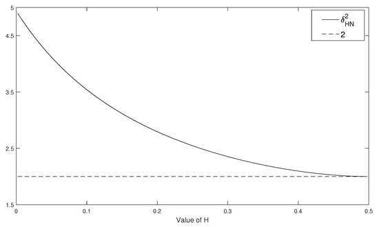
Following Hu et al. (2019), Xiao and Yu (2019b) considered the ergodic-type estimate of κ defined in (25) when $0<H<1/2$ and showed that:

$$\sqrt{T}\left({\widehat{\kappa }}_{HN}-\kappa \right)\stackrel{d}{\to }\mathcal{N}\left(0,\kappa {\delta }_{HN}^2\right),$$

(40)

where ${\delta }_{HN}^2=\frac{1}{4H^2}\left[\left(4H-1\right)+\frac{2\Gamma \left(2-4H\right)\Gamma \left(4H\right)}{\Gamma \left(2H\right)\Gamma \left(1-2H\right)}\right]$. Figure 1 compares the asymptotic variances of ${\tilde{\kappa }}_T$ and ${\widehat{\kappa }}_{HN}$ by plotting ${\delta }_{HN}^2$ against twofor $H\in (0,1/2)$. It can be seen that ${\tilde{\kappa }}_T$ is more efficient than ${\widehat{\kappa }}_{HN}$. The smaller H is, the larger the relative asymptotic efficiency in ${\tilde{\kappa }}_T$. The two estimators have the same asymptotic variance when $H=1/2$.

Figure 1. Plots of ${\delta }_{HN}^2$ against two as functions of H.

Remark 5.

Using the Taylor expansion and Theorem 3.2 of Xiao and Yu (2019b), we can easily obtain that for $0<H<1/2$:

$$\sqrt{T}\left({\widehat{\alpha }}_{HN}-\alpha \right)\stackrel{d}{\to }\mathcal{N}\left(0,\frac{{\alpha }^2}{\kappa }{\delta }_{HN}^2\right).$$

(41)

Comparing (38) with (41), we can see that ${\tilde{\alpha }}_T$ and ${\widehat{\alpha }}_{HN}$ share the same convergence rate. However, ${\tilde{\alpha }}_T$ is more efficient than ${\widehat{\alpha }}_{HN}$ because ${\delta }_{HN}^2<2$ for $H\in (0,1/2)$.

3.2. Asymptotic Theory When $H=1/2$

When $H=1/2$, $B_t^{1/2}=W_t$, which is a standard Brownian motion, and the fVm becomes the standard Vasicek model. In this case, it can be shown that fundamental martingale $M_t^H$ becomes a standard Brownian motion. Consequently, the MLE reduces to the LS estimates and can be rewritten as:

$$\begin{array}{ccc}\hfill {\tilde{\alpha }}_T& =& \frac{X_T{\int }_0^T{X}_t^{2}dt-{\int }_0^T{X}_{t}dt{\int }_0^T{X}_{t}d{X}_t}{T{\int }_0^T{X}_t^{2}dt-{\left({\int }_0^T{X}_{t}dt\right)}^2},\hfill \end{array}$$

(42)

$$\begin{array}{ccc}\hfill {\tilde{\kappa }}_T& =& \frac{X_T{\int }_0^T{X}_{t}dt-T{\int }_0^T{X}_{t}d{X}_t}{T{\int }_0^T{X}_t^{2}dt-{\left({\int }_0^T{X}_{t}dt\right)}^2},\hfill \end{array}$$

(43)

where the stochastic integration ${\int }_0^T{X}_{t}d{X}_t$ is interpreted as an Itô integral. The asymptotic theory in (42) and (43) has been studied in the literature; see, for example, Kubilius et al. (2018) and Kutoyants (2004). From page 64 of Kutoyants (2004), we can easily show that ${\tilde{\alpha }}_T$ and ${\tilde{\kappa }}_T$ are consistent and asymptotically normally distributed. Hence, we only provide the asymptotic laws of ${\tilde{\alpha }}_T$ and ${\tilde{\kappa }}_T$ for $H=1/2$ without proof.

Theorem 2.

For $\kappa >0$ and $H=1/2$ in Model (3), as $T\to \infty$, we have:

$$\begin{array}{ccc}\hfill \sqrt{T}\left({\tilde{\alpha }}_T-\alpha \right)& \stackrel{d}{\to }& \mathcal{N}\left(0,{\sigma }^2+\frac{2{\alpha }^2}{\kappa }\right),\hfill \end{array}$$

(44)

$$\begin{array}{ccc}\hfill \sqrt{T}\left({\tilde{\kappa }}_T-\kappa \right)& \stackrel{d}{\to }& \mathcal{N}\left(0,2\kappa \right).\hfill \end{array}$$

(45)

Remark 6.

When $\alpha \ne 0$, we can summarize the three sets of asymptotic theory for the MLE of α as follows:

$$\begin{array}{ccc}\hfill \mathit{If}H\in (0,1/2),\sqrt{T}\left({\tilde{\alpha }}_T-\alpha \right)& \stackrel{d}{\to }& \mathcal{N}\left(0,\frac{2{\alpha }^2}{\kappa }\right),\hfill \\ \hfill \mathit{If}H=1/2,\sqrt{T}\left({\tilde{\alpha }}_T-\alpha \right)& \stackrel{d}{\to }& \mathcal{N}\left(0,{\sigma }^2+\frac{2{\alpha }^2}{\kappa }\right),\hfill \\ \hfill \mathrm{If}H\in (1/2,1),T^{1-H}\left({\tilde{\alpha }}_T-\alpha \right)& \stackrel{d}{\to }& \mathcal{N}\left(0,{\lambda }_H{\sigma }^2\right),\hfill \end{array}$$

where the last asymptotic theory was obtained in Theorem 3.4 of Lohvinenko and Ralchenko (2017). While the three sets of asymptotic theory for ${\tilde{\kappa }}_T$ are identical, the three sets of asymptotic theory for ${\tilde{\alpha }}_T$ are different. When H changes from a value in $(0,1/2)$ to $1/2$, while the rate of convergence stays the same (i.e., $\sqrt{T}$), the asymptotic variance changes from $\frac{2{\alpha }^2}{\kappa }$ to ${\sigma }^2+\frac{2{\alpha }^2}{\kappa }$. When H changes from a value in $(0,1/2]$ to $(1/2,1)$, both the rate of convergence and the asymptotic variance change.

Remark 7.

When α is known and assumed to be zero and $H=1/2$, the asymptotic theory for the MLE of κ was obtained in Brown and Hewitt (1975) and in Feigin (1976). The two sets of asymptotic theory are the same, suggesting that there is no efficiency loss in estimating κ when α is estimated or not.

4. Asymptotic Theory When $\mathbf{\kappa }=\mathbf{0}$

In this section, we consider the asymptotic laws of ${\tilde{\alpha }}_T$ and ${\tilde{\kappa }}_T$ for the entire range for the Hurst parameter, i.e., $H\in (0,1)$. Note that when $\kappa =0$, we have:

$$X_t=X_0+\alpha t+\sigma B_t^H.$$

(46)

For the model $d{U}_t=-\kappa U_{t}dt+d{B}_t^H$, it is well known that the MLE of $\kappa$ can be expressed as:

$${\widehat{\kappa }}_T-\kappa =\frac{-{\int }_0^T{\widehat{P}}_H\left(t\right)d{M}_t^H}{{\int }_0^T{\widehat{P}}_H^2\left(t\right)d{\omega }_t^H},$$

(47)

where ${\widehat{P}}_H\left(t\right)=\frac{d}{d{\omega }_t^H}{\int }_0^t{k}_H\left(t,s\right)B_s^{H}ds$.

Before considering the asymptotic properties of ${\tilde{\alpha }}_T$ and ${\tilde{\kappa }}_T$, we first introduce a lemma, which will be used to derive the asymptotic theory.

Lemma 2.

For $\kappa =0$ and $H\in \left(0,1\right)$ in Model (1), as $T\to \infty$, we have:

$$\begin{array}{ccc}\hfill {\int }_0^T{\widehat{P}}_H\left(t\right)d{M}_t^H& =& O_p\left(T\right),\hfill \end{array}$$

(48)

$$\begin{array}{ccc}\hfill {\int }_0^T{\widehat{P}}_H^2\left(t\right)d{\omega }_t^H& =& O_p\left(T^2\right),\hfill \end{array}$$

(49)

$$\begin{array}{ccc}\hfill {\int }_0^{T}td{\omega }_t^H& =& \frac{1}{{\lambda }_H}\frac{2-2H}{3-2H}{T}^{3-2H},\hfill \end{array}$$

(50)

$$\begin{array}{ccc}\hfill {\int }_0^T{t}^{2}d{\omega }_t^H& =& \frac{1}{{\lambda }_H}\frac{1-H}{2-H}{T}^{4-2H},\hfill \end{array}$$

(51)

$$\begin{array}{ccc}\hfill {\int }_0^T{\widehat{P}}_H\left(t\right)d{\omega }_t^H& =& O_p\left(T^{2-H}\right),\hfill \end{array}$$

(52)

$$\begin{array}{ccc}\hfill {\int }_0^{T}t{\widehat{P}}_H\left(t\right)d{\omega }_t^H& =& O_p\left(T^{3-H}\right),\hfill \end{array}$$

(53)

$$\begin{array}{ccc}\hfill V_H\left(T\right)& =& \frac{{\lambda }_H}{k_H}B\left(\frac{3}{2}-H,\frac{3}{2}-H\right),\hfill \end{array}$$

(54)

$$\begin{array}{ccc}\hfill \frac{d}{d{\omega }_t^H}{\int }_0^t{k}_H\left(t,s\right)sds& =& a_{H}t,\hfill \end{array}$$

(55)

where $B(·,·)$ is the Beta function, ${\lambda }_H$ is defined by (8), and $a_H=\frac{3-2H}{4\left(1-H\right)}$.

We can now describe the asymptotic behavior of ${\tilde{\alpha }}_T$ and ${\tilde{\kappa }}_T$ as $T\to \infty$.

Theorem 3.

For $\kappa =0$, $\alpha \ne 0$, and $H\in \left(0,1\right)$ in Model (1), as $T\to \infty$, we have:

$$\begin{array}{ccc}\hfill T^{1-H}\left({\tilde{\alpha }}_T-\alpha \right)& \stackrel{d}{\to }& \mathcal{N}\left(0,{\sigma }^2{\rho }_H\right),\hfill \end{array}$$

(56)

$$\begin{array}{ccc}\hfill T^{2-H}\left({\tilde{\kappa }}_T-\kappa \right)& \stackrel{d}{\to }& \mathcal{N}\left(0,\frac{{\sigma }^2}{{\alpha }^2}{\varphi }_H\right),\hfill \end{array}$$

(57)

where ${\rho }_H={\lambda }_H{\left(3-2H\right)}^2$, ${\varphi }_H=\frac{32H(1-H)(2-H)\Gamma (3-2H)\Gamma (H+\frac{1}{2})}{\Gamma (\frac{3}{2}-H)}$ and ${\lambda }_H$ is defined by (8).

Remark 8.

In the case of $H=1/2$ and $\alpha \ne 0$, we can see that $X_t=X_0+\alpha t+\sigma W_t$. A straightforward algebraic calculation shows ${\omega }_t^H=t,P_H\left(t\right)=\frac{1}{\sigma }{X}_t$, $M_T^H=W_t$, ${\widehat{P}}_H\left(t\right)=W_t$ and that:

$$\begin{array}{ccc}\hfill \frac{1}{T^3}{\int }_0^T{X}_t^{2}dt& =& \frac{{\alpha }^2}{3}+o_p\left(1\right),\hfill \end{array}$$

(58)

$$\begin{array}{ccc}\hfill \frac{1}{T^2}{\int }_0^T{X}_{t}dt& =& \frac{\alpha }{2}+o_p\left(1\right),\hfill \end{array}$$

(59)

$$\begin{array}{ccc}\hfill \frac{1}{T\sqrt{T}}{\int }_0^T{X}_{t}d{W}_t& =& \frac{\alpha }{T\sqrt{T}}{\int }_0^{T}td{W}_t+o_p\left(1\right).\hfill \end{array}$$

(60)

Then, by the scaling properties of the Brownian motion, (21) and (58)–(60), we deduce that:

$$\begin{array}{ccc}\sqrt{T}\left({\tilde{\alpha }}_T-\alpha \right)\hfill & =& \sqrt{T}\left(\frac{W_T{\int }_0^T{X}_t^{2}dt-{\int }_0^T{X}_{t}d{W}_t{\int }_0^T{X}_{t}dt}{T{\int }_0^T{X}_t^{2}dt-{\left({\int }_0^T{X}_{t}dt\right)}^2}\sigma \right)\hfill \\ & =& \sqrt{T}\left(\frac{1}{\sqrt{T}}\frac{\frac{1}{\sqrt{T}}{W}_T\frac{1}{T^3}{\int }_0^T{X}_t^{2}dt-\frac{1}{T\sqrt{T}}{\int }_0^T{X}_{t}d{W}_t\frac{1}{T^2}{\int }_0^T{X}_{t}dt}{\frac{1}{T^3}{\int }_0^T{X}_t^{2}dt-{\left(\frac{1}{T^2}{\int }_0^T{X}_{t}dt\right)}^2}\sigma \right)\hfill \\ & =& \frac{\frac{{\alpha }^2}{3}\frac{W_T}{\sqrt{T}}-\frac{{\alpha }^2}{2}\frac{1}{T\sqrt{T}}{\int }_0^{T}td{W}_t+o_p\left(1\right)}{\frac{{\alpha }^2}{3}-{\left(\frac{\alpha }{2}\right)}^2+o_p\left(1\right)}\sigma \hfill \\ & =& 12\sigma \left(\frac{W_T}{3\sqrt{T}}-\frac{1}{2T\sqrt{T}}{\int }_0^{T}td{W}_t\right)+o_p\left(1\right)\hfill \\ & \stackrel{d}{\to }& \mathcal{N}\left(0,4{\sigma }^2\right),\hfill \end{array}$$

which is identical to (56) with $H=1/2$. Moreover, using (22) and (58)–(60), we can write:

$$\begin{array}{ccc}T\sqrt{T}\left({\tilde{\kappa }}_T-\kappa \right)\hfill & =& T\sqrt{T}\left[\frac{\left(W_T{\int }_0^T{X}_{t}dt-T{\int }_0^T{X}_{t}d{W}_t\right)\sigma }{T{\int }_0^T{X}_t^{2}dt-{\left({\int }_0^T{X}_{t}dt\right)}^2}\right]\hfill \\ & =& \frac{\left[\frac{W_T}{\sqrt{T}}\frac{1}{T^2}{\int }_0^T{X}_{t}dt-\frac{1}{T\sqrt{T}}{\int }_0^T{X}_{t}d{W}_t\right]\sigma }{\frac{1}{T^3}{\int }_0^T{X}_t^{2}dt-{\left(\frac{1}{T^2}{\int }_0^T{X}_{t}dt\right)}^2}\hfill \\ & \stackrel{d}{\to }& \mathcal{N}\left(0,\frac{12{\sigma }^2}{{\alpha }^2}\right),\hfill \end{array}$$

which is identical to (57) with $H=1/2$ being assumed.

Remark 9.

In the case of $H=1/2$ and $\alpha =0$, with α and κ being estimated, by the scaling properties of the Brownian motion, we have:

$$\begin{array}{ccc}\hfill \sqrt{T}\left({\tilde{\alpha }}_T-\alpha \right)& \stackrel{d}{\to }& \frac{W_1{\left({\int }_0^1{W}_{t}dt\right)}^2-{\int }_0^1{W}_{t}dt{\int }_0^1{W}_{t}d{W}_t}{{\int }_0^1{W}_t^{2}dt-{\left({\int }_0^1{W}_{t}dt\right)}^2}\sigma ,\hfill \\ \hfill T\left({\tilde{\kappa }}_T-\kappa \right)& \stackrel{d}{\to }& \frac{W_1{\int }_0^1{W}_{t}dt-{\int }_0^1{W}_{t}d{W}_t}{{\int }_0^1{W}_t^{2}dt-{\left({\int }_0^1{W}_{t}dt\right)}^2}.\hfill \end{array}$$

Thus, the limiting distributions of ${\tilde{\alpha }}_T$ and ${\tilde{\kappa }}_T$ are not normal. In particular, the asymptotic distribution of ${\tilde{\kappa }}_T$ is a Dickey–Fuller–Phillips-type distribution with the rate of convergence being T. Hence, when $\kappa =0$ is unknown, the value of α plays an important role in the study of asymptotic laws for the MLE.

5. Asymptotic Theory When $\mathbf{\kappa }<\mathbf{0}$

When $\kappa <0$, the model given by (3) is non-ergodic or explosive. Since the proofs of the asymptotic theory of ${\tilde{\alpha }}_T$ and ${\tilde{\kappa }}_T$ when $H=1/2$ are different from those when $H\in (0,1/2)\cup (1/2,1)$, we first consider the case of $H=1/2$. For the sake of notational simplicity, we introduce the process ${\xi }_t=\sigma {\int }_0^t{e}^{\kappa s}d{W}_s\sim \mathcal{N}\left(0,\frac{{\sigma }^2\left(e^{2\kappa t}-1\right)}{2\kappa }\right)$ for $t\ge 0$. Obviously, ${\xi }_{\infty }\sim \mathcal{N}\left(0,-\frac{{\sigma }^2}{2\kappa }\right)$. Moreover, using (17) and the definition of ${\xi }_t$, we can easily obtain:

$$\begin{array}{ccc}\hfill \sigma e^{\kappa T}{\int }_0^T{U}_{t}dt=e^{\kappa T}{\int }_0^T{e}^{-\kappa t}{\xi }_{t}dt& \stackrel{p}{\to }& -\frac{{\xi }_{\infty }}{\kappa },\hfill \end{array}$$

(61)

$$\begin{array}{ccc}\hfill \sigma e^{2\kappa T}{\int }_0^T{e}^{-\kappa t}{U}_{t}dt& \stackrel{p}{\to }& -\frac{{\xi }_{\infty }}{2\kappa }.\hfill \end{array}$$

(62)

Since $\mathbb{E}\left[{\left({\int }_0^T{e}^{\kappa \left(T-t\right)}d{W}_t\right)}^2\right]=e^{2\kappa T}{\int }_0^T{e}^{-2\kappa t}dt=\frac{e^{2\kappa T}-1}{2\kappa }$, we can obtain:

$${\int }_0^T{e}^{\kappa \left(T-t\right)}d{W}_t=O_p\left(1\right).$$

(63)

Moreover, let ${\eta }_t=\sigma {\int }_0^t{e}^{\kappa \left(t-s\right)}d{W}_s$ be a zero mean Gaussian process. Since $\mathbb{E}\left[{\eta }_t^2\right]={\sigma }^2{\int }_0^t{e}^{2\kappa \left(t-s\right)}ds=-\frac{{\sigma }^2}{2\kappa }+\frac{{\sigma }^2}{2\kappa }{e}^{2\kappa t}$, we have ${\eta }_{\infty }\sim \mathcal{N}\left(0,-\frac{{\sigma }^2}{2\kappa }\right)$. Consequently, we can obtain:

$$\sigma {\int }_0^T{e}^{\kappa \left(T-t\right)}{\xi }_{t}d{W}_t\stackrel{p}{\to }{\xi }_{\infty }{\eta }_{\infty },$$

(64)

where ${\xi }_{\infty }$ and ${\eta }_{\infty }$ are two independent $N(0,-{\sigma }^2/\left(2\kappa \right))$ random variables.

5.1. Asymptotic Theory When $H=1/2$

Now, we can state the key results of the asymptotic theory for ${\tilde{\alpha }}_T$ and ${\tilde{\kappa }}_T$ when $H=1/2$.

Theorem 4.

For $\kappa <0$, $H=1/2$ in Model (1), as $T\to \infty$, we have:

$$\begin{array}{ccc}\hfill \sqrt{T}\left({\tilde{\alpha }}_T-\alpha \right)& \stackrel{d}{\to }& \mathcal{N}\left(0,{\sigma }^2\right),\hfill \end{array}$$

(65)

$$\begin{array}{ccc}\hfill \frac{e^{-\kappa T}}{2\kappa }\left({\tilde{\kappa }}_T-\kappa \right)& \stackrel{d}{\to }& \frac{{\eta }_{\infty }}{X_0-\frac{\alpha }{\kappa }+{\xi }_{\infty }},\hfill \end{array}$$

(66)

where ${\xi }_{\infty }$ and ${\eta }_{\infty }$ are two independent $\mathcal{N}(0,-{\sigma }^2/\left(2\kappa \right))$ random variables.

Remark 10.

In (66), if we set $X_0=\frac{\alpha }{\kappa }$, the limiting distribution of $\frac{e^{-\kappa T}}{2\kappa }\left({\tilde{\kappa }}_T-\kappa \right)$ becomes a standard Cauchy variate. This limiting distribution is the same as that in the Vasicek model driven by a standard Brownian motion (see, e.g., Feigin 1976). The asymptotic theory in (66) is similar to that in the explosive discrete-time and continuous-time models when discretely-sampled data are available (see, e.g., White 1958; Anderson 1959; Phillips and Magdalinos 2007; Wang and Yu 2015, 2016).

5.2. Asymptotic Theory When $H\in (0,1/2)\cup (1/2,1)$

We now turn to the case when $H\in (0,1/2)\cup (1/2,1)$ assuming $\kappa <0$. The limiting theory is the most difficult to derive in our paper and, hence, is the main technical contribution to the literature. First, we can have the following lemma.

Lemma 3.

For $\kappa <0$ and $H\in (0,1)$ in Model (1), we have:

$$\begin{array}{ccc}\hfill V_H\left(t\right)& =& O\left(t^{H-\frac{1}{2}}{e}^{-\kappa t}\right),\hfill \end{array}$$

(67)

$$\begin{array}{ccc}\hfill {\int }_0^T{\tilde{P}}_H^2\left(t\right)d{\omega }_t^H& =& O_p\left(e^{-2\kappa T}\right),\hfill \end{array}$$

(68)

$$\begin{array}{ccc}\hfill {\int }_0^T{\tilde{P}}_H\left(t\right)d{M}_t^H& =& O_p\left(e^{-\kappa T}\right),\hfill \end{array}$$

(69)

$$\begin{array}{ccc}\hfill {\int }_0^T{V}_H\left(t\right)d{\omega }_t^H& =& O\left(T^{\frac{1}{2}-H}{e}^{-\kappa T}\right),\hfill \end{array}$$

(70)

$$\begin{array}{ccc}\hfill {\int }_0^T{\tilde{P}}_H\left(t\right)d{\omega }_t^H& =& O_p\left(e^{-\kappa T}{T}^{\frac{1}{2}-H}\right),\hfill \end{array}$$

(71)

$$\begin{array}{ccc}\hfill {\int }_0^T{V}_H^2\left(t\right)d{\omega }_t^H& =& O\left(e^{-2\kappa T}\right),\hfill \end{array}$$

(72)

$$\begin{array}{ccc}\hfill {\int }_0^T{V}_H\left(t\right){\tilde{P}}_H\left(t\right)d{\omega }_t^H& =& O_p\left(e^{-2\kappa T}\right),\hfill \end{array}$$

(73)

$$\begin{array}{ccc}\hfill {\int }_0^T{V}_H\left(t\right)d{M}_t^H& =& O_p\left(e^{-\kappa T}\right).\hfill \end{array}$$

(74)

Now, we can state the asymptotic theory for ${\tilde{\alpha }}_T$ and ${\tilde{\kappa }}_T$ for $\kappa <0$ and $H\in (0,1/2)\cup (1/2,1)$.

Theorem 5.

When $\kappa <0$, $H\in (0,1/2)\cup (1/2,1)$, and $X_0=\frac{\alpha }{\kappa }$ in Model (1), as $T\to \infty$, we have:

$$\begin{array}{ccc}\hfill T^{1-H}\left({\tilde{\alpha }}_T-\alpha \right)& \stackrel{d}{\to }& \mathcal{N}\left(0,{\lambda }_H{\sigma }^2\right),\hfill \end{array}$$

(75)

$$\begin{array}{ccc}\hfill \frac{e^{-\kappa T}}{2\kappa }\left({\tilde{\kappa }}_T-\kappa \right)& \stackrel{d}{\to }& \frac{X\sqrt{sin\left(\pi H\right)}}{Y},\hfill \end{array}$$

(76)

where X and Y are two independent $\mathcal{N}(0,1)$ random variables.

Remark 11.

For the entire range of $H\in (0,1)$, the asymptotic distribution of ${\tilde{\alpha }}_T$ is normal with the rate of convergence of $T^{1-H}$ and variance ${\sigma }^2$. This asymptotic distribution is the same as that of the LS estimate (see Theorem 3.5 in Xiao and Yu (2019a) and Section 3 in Xiao and Yu (2019b)).

Remark 12.

According to (76), the asymptotic law of $\frac{e^{-\kappa T}}{2\kappa }\left({\tilde{\kappa }}_T-\kappa \right)$ is the standard Cauchy times $\sqrt{sin\left(\pi H\right)}$. For $H\in (0,1/2)\cup (1/2,1)$, $\sqrt{sin\left(\pi H\right)}\in (0,1)$, suggesting that as H draws further away from $1/2$, κ is estimated with higher accuracy. Moreover, with $X_0=\frac{\alpha }{\kappa }$, from Theorem 3.5 in Xiao and Yu (2019a, 2019b), we can see that the LS estimator of κ, which is denoted by ${\widehat{\kappa }}_{LS}$, has the asymptotic law $\frac{e^{-\kappa T}}{2\kappa }\left({\widehat{\kappa }}_{LS}-\kappa \right)\stackrel{d}{\to }C$, where C is the standard Cauchy distribution. Since the second moment of the Cauchy distribution is infinite, we cannot use the variances to measure the asymptotic relative efficiency. From Theorem 2 in Tanaka (2020) and based on the asymptotic concentration probability, we can see that the MLE is always more efficient asymptotically than the LS estimator for $H\in (0,0.5)\cup (0.5,1)$. For $H=1/2$, the MLE is asymptotically the same as the LS estimator.

Remark 13.

When $X_0\ne \frac{\alpha }{\kappa }$, using Lemma 3, we can obtain:

$$\begin{array}{ccc}\hfill \frac{e^{-\kappa T}}{2\kappa }\left({\tilde{\kappa }}_T-\kappa \right)& =& \frac{-2\kappa e^{\kappa T}{\int }_0^T\left[\frac{1}{\sigma }\left(X_0-\frac{\alpha }{\kappa }\right)V_H\left(t\right)+{\tilde{P}}_H\left(t\right)\right]d{M}_t^H+o_p\left(1\right)}{4{\kappa }^2{e}^{2\kappa T}{\int }_0^T{\left[\frac{1}{\sigma }\left(X_0-\frac{\alpha }{\kappa }\right)V_H\left(t\right)+{\tilde{P}}_H\left(t\right)\right]}^{2}d{\omega }_t^H+o_p\left(1\right)}.\hfill \end{array}$$

In this case, to obtain the asymptotic distribution of $e^{-\kappa T}\left({\tilde{\kappa }}_T-\kappa \right)/\left(2\kappa \right)$, one needs to calculate the Laplace transform of ${\int }_0^T{\left[\frac{1}{\sigma }\left(X_0-\frac{\alpha }{\kappa }\right)V_H\left(t\right)+{\tilde{P}}_H\left(t\right)\right]}^{2}d{\omega }_t^H$. On the other hand, for $1/2<H<1$, using the moment generating function of $S_T$, ${\int }_0^T{P}_H^2\left(t\right)d{\omega }_t^H$, ${\int }_0^T{P}_H\left(t\right)d{S}_t$, and ${\int }_0^T{P}_H\left(t\right)d{\omega }_t^H$, Lohvinenko and Ralchenko (2019) provided the joint asymptotic normality of MLE of the vector parameter $(\alpha ,\kappa )$:

$$\begin{array}{ccc}\hfill \left(\begin{array}{c}{T}^{1-H}\left({\tilde{\alpha }}_T-\alpha \right)\\ e^{-\kappa T}\left({\tilde{\kappa }}_T-\kappa \right)\end{array}\right)& \stackrel{d}{\to }& \left(\begin{array}{c}{\vartheta }_1\hfill \\ {\vartheta }_2/{\vartheta }_3\hfill \end{array}\right),\hfill \end{array}$$

where ${\vartheta }_1\stackrel{d}{\to }\mathcal{N}\left(0,{\lambda }_H{\sigma }^2\right)$, ${\vartheta }_2\stackrel{d}{\to }\mathcal{N}\left(0,1\right)$, and ${\vartheta }_3\stackrel{d}{\to }\mathcal{N}\left(\frac{\left(x_0-\frac{\alpha }{\kappa }\right)\sqrt{{\lambda }_H}{\rho }_H{\left(-\kappa \right)}^{H-1}}{\sqrt{\pi \left(4-4H\right)}},\frac{1}{4{\kappa }^{2}sin\left(\pi H\right)}\right)$, which generalizes (76) for particular $X_0=\alpha /\kappa$.

6. Concluding Remarks and Future Directions

The fVm has found more and more applications in practice. In this paper, we consider the MLE of parameters in the drift term when a continuous record of observations is available. The ML estimation is made possible due to the presence of the fundamental martingale and the generalized Girsanov theorem. The asymptotic theory is based on the assumption that $T\to \infty$.

It is shown that the MLE of $\alpha$ is asymptotically normal regardless of the sign of $\kappa$. However, the asymptotic law of the MLE of $\kappa$ critically depends on the sign of $\kappa$. More precisely, when $\kappa >0$ and $H\in (0,1)$, we have shown that the asymptotic distribution of the MLE of $\kappa$ is normal with the rate of convergence being $\sqrt{T}$. The asymptotic variance is $2\kappa$, which is independent of H. When $\kappa =0$ and $\alpha \ne 0$, the asymptotic distribution of the MLE of $\kappa$ is normal with the rate of convergence being $T^{2-H}$. The asymptotic variance depends on H. When $\kappa =0$ and $\alpha =0$, the asymptotic distribution of the MLE of $\kappa$ is a Dickey–Fuller–Phillips distribution with the rate of convergence being T. When $\kappa <0$, it is shown that the limiting distribution is a Cauchy-type with the rate of convergence being $e^{-\kappa T}$. If one further assumes that $X_0=\alpha /\kappa$, the limiting distribution becomes a standard Cauchy variate multiplied by $\sqrt{sin\left(\pi H\right)}$. Table 1 summarizes the asymptotic laws of ${\tilde{\alpha }}_T$ and ${\tilde{\kappa }}_T$ for different ranges of H and $\kappa$, where ${\lambda }_H=\frac{2H\Gamma \left(3-2H\right)\Gamma \left(H+\frac{1}{2}\right)}{\Gamma \left(\frac{3}{2}-H\right)}$, ${\rho }_H={\lambda }_H{\left(3-2H\right)}^2$, ${\varphi }_H=\frac{32H(1-H)(2-H)\Gamma (3-2H)\Gamma (H+\frac{1}{2})}{\Gamma (\frac{3}{2}-H)}$, ${\xi }_{\infty }$, and ${\eta }_{\infty }$ are two independent $\mathcal{N}(0,-{\sigma }^2/\left(2\kappa \right))$ random variables and X and Y are two independent $\mathcal{N}(0,1)$ random variables. Moreover, we assume $X_0=\alpha /\kappa$ for $\kappa <0$ and $H\in (0,1/2)\cup (1/2,1)$.

Table 1. Summary of the asymptotic laws of ${\tilde{\alpha }}_T$ and ${\tilde{\kappa }}_T$ for different ranges of H and $\kappa$.

	$0<\mathit{H}<1/2$	$\mathit{H}=1/2$	$1/2<\mathit{H}<1$
$\kappa >0$	$\sqrt{T}\left({\tilde{\alpha }}_T-\alpha \right)\stackrel{d}{\to }\mathcal{N}\left(0,\frac{2{\alpha }^2}{\kappa }\right)$	$\sqrt{T}\left({\tilde{\alpha }}_T-\alpha \right)\stackrel{d}{\to }\mathcal{N}\left(0,{\sigma }^2+\frac{2{\alpha }^2}{\kappa }\right)$	$T^{1-H}\left({\tilde{\alpha }}_T-\alpha \right)\stackrel{d}{\to }\mathcal{N}\left(0,{\lambda }_H{\sigma }^2\right)$
	$\sqrt{T}\left({\tilde{\kappa }}_T-\kappa \right)\stackrel{d}{\to }\mathcal{N}\left(0,2\kappa \right)$	$\sqrt{T}\left({\tilde{\kappa }}_T-\kappa \right)\stackrel{d}{\to }\mathcal{N}\left(0,2\kappa \right)$	$\sqrt{T}\left({\tilde{\kappa }}_T-\kappa \right)\stackrel{d}{\to }\mathcal{N}\left(0,2\kappa \right)$
$\kappa =0$	$T^{1-H}\left({\tilde{\alpha }}_T-\alpha \right)\stackrel{d}{\to }\mathcal{N}\left(0,{\sigma }^2{\rho }_H\right)$	$\sqrt{T}\left({\tilde{\alpha }}_T-\alpha \right)\stackrel{d}{\to }\mathcal{N}\left(0,4{\sigma }^2\right)$	$T^{1-H}\left({\tilde{\alpha }}_T-\alpha \right)\stackrel{d}{\to }\mathcal{N}\left(0,{\sigma }^2{\rho }_H\right)$
	$T^{2-H}\left({\tilde{\kappa }}_T-\kappa \right)\stackrel{d}{\to }\mathcal{N}\left(0,\frac{{\sigma }^2}{{\alpha }^2}{\varphi }_H\right)$	$T^{3/2}\left({\tilde{\kappa }}_T-\kappa \right)\stackrel{d}{\to }\mathcal{N}\left(0,\frac{12{\sigma }^2}{{\alpha }^2}\right)$	$T^{2-H}\left({\tilde{\kappa }}_T-\kappa \right)\stackrel{d}{\to }\mathcal{N}\left(0,\frac{{\sigma }^2}{{\alpha }^2}{\varphi }_H\right)$
$\kappa <0$	$T^{1-H}\left({\tilde{\alpha }}_T-\alpha \right)\stackrel{d}{\to }\mathcal{N}\left(0,{\lambda }_H{\sigma }^2\right)$	$\sqrt{T}\left({\tilde{\alpha }}_T-\alpha \right)\stackrel{d}{\to }\mathcal{N}\left(0,{\sigma }^2\right)$	$T^{1-H}\left({\tilde{\alpha }}_T-\alpha \right)\stackrel{d}{\to }\mathcal{N}\left(0,{\lambda }_H{\sigma }^2\right)$
	$\frac{e^{-\kappa T}}{2\kappa }\left({\tilde{\kappa }}_T-\kappa \right)\stackrel{d}{\to }\frac{X\sqrt{sin\left(\pi H\right)}}{Y}$	$\frac{e^{-\kappa T}}{2\kappa }\left({\tilde{\kappa }}_T-\kappa \right)\stackrel{d}{\to }\frac{{\eta }_{\infty }}{X_0-\frac{\alpha }{\kappa }+{\xi }_{\infty }}$	$\frac{e^{-\kappa T}}{2\kappa }\left({\tilde{\kappa }}_T-\kappa \right)\stackrel{d}{\to }\frac{X\sqrt{sin\left(\pi H\right)}}{Y}$

This study also suggests several important directions for future research. First, it is worth investigating generalizing the results in this paper to nonlinear stochastic differential equations driven by the fBm. The ergodic theorem, fractional calculus, and Malliavin calculus will be employed for obtaining the asymptotic properties of both the MLE and the LS estimators.

Second, in this paper, H and $\sigma$ are assumed to be known. In practice, both H and $\sigma$ are almost always unknown. Although many approaches have been proposed to estimate the Hurst coefficient and the volatility parameter from discrete time observations, how to estimate H and $\sigma$ in fVm with a continuous record of observations is an open question. It is interesting to realize that we can use the generalized quadratic variation to estimate both the Hurst parameter and the volatility parameter in fVm. For $T>0$ and any $ϵ\ne \xi$,

$$H=\underset{ϵ\downarrow 0,\xi \downarrow 0}{lim}\frac{1}{2}log\left(\frac{ϵ}{\xi }\right)log\left(\frac{{\int }_0^T{\left(X_{t+\xi }-X_t\right)}^{2}dt}{{\int }_0^T{\left(X_{t+ϵ}-X_t\right)}^{2}dt}\right),{\sigma }^2=\frac{{lim}_{ϵ\downarrow 0}{\int }_0^T{\left(X_{t+ϵ}-X_t\right)}^{2}dt}{{ϵ}^{2H}T}.$$

It would be interesting to study the asymptotic properties of these estimators mentioned above, which will be reported in later work.

Third, this paper assumes that a continuous record of an increasing time span is available for the development of asymptotic theory. In practice, data are typically observed at discrete time points with $(0,h,2h,\cdots ,Nh(:=T\left)\right)$ where h is the sampling interval and T is the time span. When high frequency data over a long spanning time period are available, one may consider using a double asymptotic scheme by assuming $h\to 0$ and $T\to \infty$. The discretized model corresponding to (3) is given by:

$$y_{th}=\mu +exp(-\kappa h)\left(y_{\left(t-1\right)h}-\mu \right)+u_t,{(1-L)}^d{u}_t={\epsilon }_t,t=1,\cdots ,N,$$

where L is the lag operator, $d=H-1/2$. As shown in Wang and Yu (2016), under the double asymptotic scheme, $exp(-\kappa h)=exp\left\{-\kappa /k_N\right\}=1-\kappa /k_N+O\left(k_N^{-2}\right)\to 1$ where $k_N:=1/h\to \infty$ as $h\to 0$ and $k_N/N=1/T\to 0$ as $T\to \infty$. This implies an autoregressive (AR) model with the AR root moderately deviating from unity and with a fractionally integrated error term with $d\in (-1/2,0)$. This model is closely related to a model considered in Magdalinos (2012) where it is assumed that $d\in (0,1/2)$. Developing double asymptotic theory based on discretely-sampled data will allow one to extend the results of Magdalinos (2012) to the case where $d\in (-1/2,1/2)$. The development of the MLE and the asymptotic theory is beyond the scope of this paper and will be reported in later work.

Appendix A.1. Proof of Lemma 1

We first consider (30). Let us introduce the modified Bessel functions of the first kind (see, e.g., Abramowitz and Stegun 1972), which are defined as:

$$I_{\nu }\left(z\right)={\left(\frac{1}{2}z\right)}^{\nu }\sum _{k=0}^{\infty }\frac{{\left(\frac{1}{4}{z}^2\right)}^k}{k!\Gamma (\nu +k+1)},\mathrm{where}\nu \in \mathbb{R}.$$

(A1)

From page 377 in Abramowitz and Stegun (1972), we can see that the asymptotic behavior of $I_{\nu }\left(z\right)$ is:

$$I_{\nu }\left(z\right)=\frac{e^z}{\sqrt{2\pi z}}[1+O(1/z)],\mathrm{when}z\to \infty ,|argz|<\frac{\pi }{2}.$$

(A2)

Using (6), (15) and (A2), we get:

$$\begin{array}{ccc}{V}_H\left(T\right)\hfill & =& \frac{d}{d{\omega }_T^H}{\int }_0^T{k}_H\left(T,s\right)e^{-\kappa s}ds\hfill \\ & =& \frac{d}{d{\omega }_T^H}\left[\frac{\sqrt{\pi }{\kappa }^{H-1}\Gamma \left(\frac{3}{2}-H\right)}{k_H}{T}^{1-H}{e}^{-\frac{\kappa T}{2}}{I}_{1-H}\left(\frac{\kappa T}{2}\right)\right]\hfill \\ & =& \frac{{\kappa }^{H-\frac{3}{2}}\Gamma \left(2-2H\right)}{\Gamma \left(\frac{1}{2}-H\right)}{T}^{H-\frac{3}{2}}+O\left(T^{H-\frac{5}{2}}\right),\hfill \end{array}$$

(A3)

which is (30).

Then, as $T\to \infty$, using arguments similar to those in Lemma 4.2 of Lohvinenko and Ralchenko (2017), we can obtain:

$${\int }_0^T{V}_H\left(t\right)d{\omega }_t^H={\int }_0^T{k}_H\left(T,s\right)e^{-\kappa s}ds=O\left(T^{\frac{1}{2}-H}\right),$$

which yields (31).

By the proof of Theorem 3 in Tanaka (2013), we can easily obtain (32) and (33). The result of (34) follows directly from ${\int }_0^1{V}_H^2\left(t\right)d{\omega }_t^H<\infty$ and ${\int }_1^T{V}_H^2\left(t\right)d{\omega }_t^H<\infty$ (see the proof of Lemma 4.7 in Lohvinenko and Ralchenko 2017).

Next, we consider (35). Let ${\tilde{J}}_T={\int }_0^T{\tilde{P}}_H\left(t\right)d{\omega }_t^H$. Then, using Lemma 2 in Lohvinenko and Ralchenko (2019) and replacing $J_T$ with ${\tilde{J}}_T$, we have:

$$\mathbb{E}\left[e^{\theta {\tilde{J}}_T}\right]={\tilde{m}}_1^{\left({\alpha }_1,{\beta }_1\right)}\left(-\frac{{\alpha }_1}{\sigma },-\kappa +{\beta }_1\right)exp\left\{\frac{{\alpha }_1^2}{2{\sigma }^2}{\omega }_T^H\right\},$$

(A4)

where ${\alpha }_1=-\sigma \theta /\kappa$, ${\beta }_1=-\kappa$, ${\tilde{m}}_1^{\left({\alpha }_1,{\beta }_1\right)}\left({\xi }_1,{\xi }_2\right)$ is the moment generating function defined by Lemma 1 in Lohvinenko and Ralchenko (2019). Using Lemma 1 in Lohvinenko and Ralchenko (2019) again, we can obtain:

$$\begin{array}{ccc}{\tilde{m}}_1^{\left({\alpha }_1,{\beta }_1\right)}\left(-\frac{{\alpha }_1}{\sigma },-\kappa +{\beta }_1\right)\hfill & =& {\left(D^{\left({\alpha }_1,{\beta }_1\right)}\left(-\kappa +{\beta }_1\right)\right)}^{-1/2}exp[\frac{\frac{{\alpha }_1^2}{{\sigma }^2}{c}_3{T}^{2-2H}{e}^{-{\beta }_{1}T}}{8D^{\left({\alpha }_1,{\beta }_1\right)}\left(-\kappa +{\beta }_1\right)}\hfill \\ & & \times I_{1-H}\left(-\frac{{\beta }_{1}T}{2}\right)I_{H-1}\left(-\frac{{\beta }_{1}T}{2}\right)-\frac{-\kappa +{\beta }_1}{2}T],\hfill \end{array}$$

(A5)

where $c_3=4(1-H)\Gamma \left(H\right)\Gamma (1-H)/{\lambda }_H$ and $D^{\left({\alpha }_1,{\beta }_1\right)}\left({\xi }_2\right)$ is defined by Equation (10) in Lohvinenko and Ralchenko (2019).

Consequently, using the fact $D^{\left({\alpha }_1,{\beta }_1\right)}\left(-\kappa +{\beta }_1\right)=e^{2\kappa T}$, ${\alpha }_1=-\sigma \theta /\kappa$, ${\beta }_1=-\kappa$, (A4) and (A5), we have:

$$\begin{array}{ccc}\mathbb{E}\left[e^{\theta {\tilde{J}}_T}\right]\hfill & =& e^{-\kappa T}exp\left[\frac{\frac{{\theta }^2}{{\kappa }^2}{c}_3{T}^{2-2H}{e}^{-{\beta }_{1}T}}{8e^{2\kappa T}}\frac{e^{\kappa T}}{\pi \kappa T}\times \left(1+O\left(T^{-1}\right)\right)-\frac{-\kappa +{\beta }_1}{2}T+\frac{{\theta }^2{\omega }_T^H}{2{\kappa }^2}\right]\hfill \\ & =& exp\left[\frac{{\theta }^2}{2{\kappa }^2}{\omega }_T^H+{\theta }^{2}O\left(T^{1-2H}\right)\right],\hfill \end{array}$$

(A6)

which yields:

$$\begin{array}{ccc}\hfill \mathbb{E}\left[{\tilde{J}}_T\right]& =& {\left.\frac{d}{d\theta }\mathbb{E}\left[e^{\theta {\tilde{J}}_T}\right]\right|}_{\theta =0}=0,\hfill \end{array}$$

(A7)

$$\begin{array}{ccc}\hfill \mathbb{E}\left[{\tilde{J}}_T^2\right]& =& {\left.\frac{d^2}{d{\theta }^2}\mathbb{E}\left[e^{\theta {\tilde{J}}_T}\right]\right|}_{\theta =0}=\frac{{\omega }_T^H}{{\kappa }^2}+O\left(T^{1-2H}\right).\hfill \end{array}$$

(A8)

Using (7), (A5), (A7) and (A8), we can obtain:

$$\begin{array}{ccc}\hfill {\tilde{J}}_T& =& O\left(T^{1-H}\right),\hfill \\ \hfill \frac{{\tilde{J}}_T}{T^{1-H}}& \stackrel{d}{\to }& \mathcal{N}\left(0,\frac{1}{{\kappa }^2{\lambda }_H}\right),\hfill \end{array}$$

which implies (35).

Now, we consider (36). Using the Cauchy–Schwarz inequality, (33) and (34), we obtain:

$$\begin{array}{ccc}{\int }_0^T{V}_H\left(t\right){\tilde{P}}_H\left(t\right)d{\omega }_t^H\hfill & \le & \sqrt{{\int }_0^T{V}_H^2\left(t\right)d{\omega }_t^H{\int }_0^T{\tilde{P}}_H^2\left(t\right)d{\omega }_t^H}\hfill \\ & =& \sqrt{O\left(1\right)O_p\left(T\right)},\hfill \end{array}$$

which implies (36).

Finally, we are left with (37). Using (34), we can obtain:

$$\mathbb{E}\left[{\left({\int }_0^T{V}_H\left(t\right)d{M}_t^H\right)}^2\right]={\int }_0^T{V}_H^2\left(t\right)d{\omega }_t^H=O\left(1\right),$$

which implies (37) directly.

Appendix A.2. Proof of Theorem 1

To simplify the notations, let ${\tilde{X}}_0:=X_0-\frac{\alpha }{\kappa }$. Using (14), we have:

$$\begin{array}{ccc}{\int }_0^T{P}_H^2\left(t\right)d{\omega }_t^H\hfill & =& {\int }_0^T{\left[\frac{\alpha }{\sigma \kappa }+\frac{1}{\sigma }{\tilde{X}}_0{V}_H\left(t\right)+{\tilde{P}}_H\left(t\right)\right]}^{2}d{\omega }_t^H\hfill \\ & =& \frac{{\alpha }^2}{{\sigma }^2{\kappa }^2}{\omega }_T^H+\frac{1}{{\sigma }^2}{\tilde{X}}_0^2{\int }_0^T{V}_H^2\left(t\right)d{\omega }_t^H+{\int }_0^T{\tilde{P}}_H^2\left(t\right)d{\omega }_t^H\hfill \\ & & +\frac{2\alpha }{{\sigma }^2\kappa }{\tilde{X}}_0{\int }_0^T{V}_H\left(t\right)d{\omega }_t^H+\frac{2\alpha }{\sigma \kappa }{\int }_0^T{\tilde{P}}_H\left(t\right)d{\omega }_t^H\hfill \\ & & +\frac{2}{\sigma }{\tilde{X}}_0{\int }_0^T{V}_H\left(t\right){\tilde{P}}_H\left(t\right)d{\omega }_t^H.\hfill \end{array}$$

(A9)

Using (14) again, we obtain:

$$\begin{array}{ccc}{\left({\int }_0^T{P}_H\left(t\right)d{\omega }_t^H\right)}^2\hfill & =& {\left[{\int }_0^T\left(\frac{\alpha }{\sigma \kappa }+\frac{1}{\sigma }{\tilde{X}}_0{V}_H\left(t\right)+{\tilde{P}}_H\left(t\right)\right)d{\omega }_t^H\right]}^2\hfill \\ & =& \frac{{\alpha }^2}{{\sigma }^2{\kappa }^2}{\left({\omega }_T^H\right)}^2+\frac{1}{{\sigma }^2}{\tilde{X}}_0^2{\left({\int }_0^T{V}_H\left(t\right)d{\omega }_t^H\right)}^2+{\left({\int }_0^T{\tilde{P}}_H\left(t\right)d{\omega }_t^H\right)}^2\hfill \\ & & +\frac{2\alpha }{\sigma \kappa }{\omega }_T^H{\int }_0^T{\tilde{P}}_H\left(t\right)d{\omega }_t^H+\frac{2\alpha }{{\sigma }^2\kappa }{\omega }_T^H{\tilde{X}}_0{\int }_0^T{V}_H\left(t\right)d{\omega }_t^H\hfill \\ & & +\frac{2}{\sigma }{\tilde{X}}_0{\int }_0^T{V}_H\left(t\right)d{\omega }_t^H{\int }_0^T{\tilde{P}}_H\left(t\right)d{\omega }_t^H.\hfill \end{array}$$

(A10)

Using (A9), (A10) and Lemma 1, we deduce that:

$$\begin{array}{cc}& {\omega }_T^H{\int }_0^T{P}_H^2\left(t\right)d{\omega }_t^H-{\left({\int }_0^T{P}_H\left(t\right)d{\omega }_t^H\right)}^2\hfill \\ =& \frac{{\omega }_T^H}{{\sigma }^2}{\tilde{X}}_0^2{\int }_0^T{V}_H^2\left(t\right)d{\omega }_t^H+{\omega }_T^H{\int }_0^T{\tilde{P}}_H^2\left(t\right)d{\omega }_t^H+{\omega }_T^H\frac{2\alpha }{{\sigma }^2\kappa }{\tilde{X}}_0{\int }_0^T{V}_H\left(t\right)d{\omega }_t^H\hfill \\ & +{\omega }_T^H\frac{2\alpha }{\sigma \kappa }{\int }_0^T{\tilde{P}}_H\left(t\right)d{\omega }_t^H+{\omega }_T^H\frac{2}{\sigma }{\tilde{X}}_0{\int }_0^T{V}_H\left(t\right){\tilde{P}}_H\left(t\right)d{\omega }_t^H\hfill \\ & -\frac{1}{{\sigma }^2}{\tilde{X}}_0^2{\left({\int }_0^T{V}_H\left(t\right)d{\omega }_t^H\right)}^2-{\left({\int }_0^T{\tilde{P}}_H\left(t\right)d{\omega }_t^H\right)}^2-\frac{2\alpha }{{\sigma }^2\kappa }{\omega }_T^H{\tilde{X}}_0{\int }_0^T{V}_H\left(t\right)d{\omega }_t^H\hfill \\ & -\frac{2\alpha }{\sigma \kappa }{\omega }_T^H{\int }_0^T{\tilde{P}}_H\left(t\right)d{\omega }_t^H-\frac{2}{\sigma }{\tilde{X}}_0{\int }_0^T{V}_H\left(t\right)d{\omega }_t^H{\int }_0^T{\tilde{P}}_H\left(t\right)d{\omega }_t^H\hfill \\ =& {\omega }_T^H{\int }_0^T{\tilde{P}}_H^2\left(t\right)d{\omega }_t^H+o_p\left(T^{3-2H}\right).\hfill \end{array}$$

(A11)

Moreover, using (14), we get:

$$\begin{array}{cc}& {\int }_0^T{P}_H\left(t\right)d{M}_t^H{\int }_0^T{P}_H\left(t\right)d{\omega }_t^H\hfill \\ =& \left[\frac{\alpha }{\sigma \kappa }{M}_T^H+\frac{1}{\sigma }{\tilde{X}}_0{\int }_0^T{V}_H\left(t\right)d{M}_t^H+{\int }_0^T{\tilde{P}}_H\left(t\right)d{M}_t^H\right]\times \hfill \\ & \left[\frac{\alpha }{\sigma \kappa }{\omega }_t^H+\frac{1}{\sigma }{\tilde{X}}_0{\int }_0^T{V}_H\left(t\right)d{\omega }_t^H+{\int }_0^T{\tilde{P}}_H\left(t\right)d{\omega }_t^H\right]\hfill \\ =& \frac{{\alpha }^2}{{\sigma }^2{\kappa }^2}{M}_T^H{\omega }_T^H+\frac{\alpha }{\sigma \kappa }{M}_T^H\frac{1}{\sigma }{\tilde{X}}_0{\int }_0^T{V}_H\left(t\right)d{\omega }_t^H+\frac{\alpha }{\sigma \kappa }{M}_T^H{\int }_0^T{\tilde{P}}_H\left(t\right)d{\omega }_t^H\hfill \\ & +\frac{1}{\sigma }{\tilde{X}}_0{\int }_0^T{V}_H\left(t\right)d{M}_t^H\frac{\alpha }{\sigma \kappa }{\omega }_T^H+\frac{1}{{\sigma }^2}{\tilde{X}}_0^2{\int }_0^T{V}_H\left(t\right)d{M}_t^H{\int }_0^T{V}_H\left(t\right)d{\omega }_t^H\hfill \\ & +\frac{1}{\sigma }{\tilde{X}}_0{\int }_0^T{V}_H\left(t\right)d{M}_t^H{\int }_0^T{\tilde{P}}_H\left(t\right)d{\omega }_t^H+\frac{\alpha }{\sigma \kappa }{\omega }_T^H{\int }_0^T{\tilde{P}}_H\left(t\right)d{M}_t^H\hfill \\ & +\frac{1}{\sigma }{\tilde{X}}_0{\int }_0^T{\tilde{P}}_H\left(t\right)d{M}_t^H{\int }_0^T{V}_H\left(t\right)d{\omega }_t^H+{\int }_0^T{\tilde{P}}_H\left(t\right)d{M}_t^H{\int }_0^T{\tilde{P}}_H\left(t\right)d{\omega }_t^H.\hfill \end{array}$$

(A12)

By combining (A9), (A12) and Lemma 1, we have:

$$\begin{array}{cc}& M_T^H{\int }_0^T{P}_H^2\left(t\right)d{\omega }_t^H-{\int }_0^T{P}_H\left(t\right)d{M}_t^H{\int }_0^T{P}_H\left(t\right)d{\omega }_t^H\hfill \\ =& \frac{{\alpha }^2}{{\sigma }^2{\kappa }^2}{M}_T^H{\omega }_T^H+\frac{M_T^H}{{\sigma }^2}{\tilde{X}}_0^2{\int }_0^T{V}_H^2\left(t\right)d{\omega }_t^H+M_T^H{\int }_0^T{\tilde{P}}_H^2\left(t\right)d{\omega }_t^H\hfill \\ & +M_T^H\frac{2\alpha }{{\sigma }^2\kappa }{\tilde{X}}_0{\int }_0^T{V}_H\left(t\right)d{\omega }_t^H+M_T^H\frac{2\alpha }{\sigma \kappa }{\int }_0^T{\tilde{P}}_H\left(t\right)d{\omega }_t^H\hfill \\ & +M_T^H\frac{2}{\sigma }{\tilde{X}}_0{\int }_0^T{V}_H\left(t\right){\tilde{P}}_H\left(t\right)d{\omega }_t^H-\frac{{\alpha }^2}{{\sigma }^2{\kappa }^2}{M}_T^H{\omega }_T^H\hfill \\ & -\frac{\alpha }{\sigma \kappa }{M}_T^H\frac{1}{\sigma }{\tilde{X}}_0{\int }_0^T{V}_H\left(t\right)d{\omega }_t^H-\frac{\alpha }{\sigma \kappa }{M}_T^H{\int }_0^T{\tilde{P}}_H\left(t\right)d{\omega }_t^H\hfill \\ & -\frac{1}{\sigma }{\tilde{X}}_0{\int }_0^T{V}_H\left(t\right)d{M}_t^H\frac{\alpha }{\sigma \kappa }{\omega }_T^H-\frac{1}{{\sigma }^2}{\tilde{X}}_0^2{\int }_0^T{V}_H\left(t\right)d{M}_t^H{\int }_0^T{V}_H\left(t\right)d{\omega }_t^H\hfill \\ & -\frac{1}{\sigma }{\tilde{X}}_0{\int }_0^T{V}_H\left(t\right)d{M}_t^H{\int }_0^T{\tilde{P}}_H\left(t\right)d{\omega }_t^H-\frac{\alpha }{\sigma \kappa }{\omega }_T^H{\int }_0^T{\tilde{P}}_H\left(t\right)d{M}_t^H\hfill \\ & -\frac{1}{\sigma }{\tilde{X}}_0{\int }_0^T{\tilde{P}}_H\left(t\right)d{M}_t^H{\int }_0^T{V}_H\left(t\right)d{\omega }_t^H-{\int }_0^T{\tilde{P}}_H\left(t\right)d{M}_t^H{\int }_0^T{\tilde{P}}_H\left(t\right)d{\omega }_t^H\hfill \\ =& -\frac{\alpha }{\sigma \kappa }{\omega }_T^H{\int }_0^T{\tilde{P}}_H\left(t\right)d{M}_t^H+o_p\left(T^{\frac{5}{2}-2H}\right).\hfill \end{array}$$

(A13)

According to Corollary 5.2 of Jost (2006), for $H<1/2$, we have the relationship between $B_t^H$ and $B_t^{1-H}$,

$$B_t^H={\left(\frac{2H}{\Gamma \left(2H\right)}\Gamma \left(3-2H\right)\right)}^{\frac{1}{2}}{\int }_0^t{\left(t-s\right)}^{2H-1}d{B}_s^{1-H}.$$

(A14)

Using (A14), following Equation (34) in Brouste and Kleptsyna (2010), we can transform Model (1) to the following model,

$$d{\widehat{X}}_t=\kappa \left(\mu -{\widehat{X}}_t\right)dt+\sigma d{B}_t^{1-H},$$

where ${\widehat{X}}_t={\left(\frac{2H}{\Gamma \left(2H\right)}\Gamma (3-2H)\right)}^{\frac{1}{2}}{\int }_0^t{(t-s)}^{1-2H}d{X}_s$. When $H<1/2$ and $1-H>1/2$, hence, the results in (4.4) and (4.5) of Lohvinenko and Ralchenko (2017) are valid for all $H\in (0,1)$.

Now, combining (21), (A13), (A11) and (4.4), (4.5) in Lohvinenko and Ralchenko (2017) with Slutsky’s theorem, we obtain:

$$\begin{array}{ccc}\sqrt{T}\left({\tilde{\alpha }}_T-\alpha \right)\hfill & =& \frac{\sqrt{T}\left[M_T^H{\int }_0^T{P}_H^2\left(t\right)d{\omega }_t^H-{\int }_0^T{P}_H\left(t\right)d{M}_t^H{\int }_0^T{P}_H\left(t\right)d{\omega }_t^H\right]}{{\omega }_T^H{\int }_0^T{P}_H^2\left(t\right)d{\omega }_t^H-{\left({\int }_0^T{P}_H\left(t\right)d{\omega }_t^H\right)}^2}\sigma \hfill \\ & =& \frac{-\frac{\alpha }{\sigma \kappa }{\omega }_T^H\frac{1}{\sqrt{T}}{\int }_0^T{\tilde{P}}_H\left(t\right)d{M}_t^H+o_p\left(T^{2-2H}\right)}{{\omega }_T^H\frac{1}{T}{\int }_0^T{\tilde{P}}_H^2\left(t\right)d{\omega }_t^H+o_p\left(T^{2-2H}\right)}\sigma \hfill \\ & \stackrel{d}{\to }& \mathcal{N}\left(0,\frac{2{\alpha }^2}{\kappa }\right).\hfill \end{array}$$

Now, we consider (39). Using (14) and (A10), we have:

$$\begin{array}{cc}& M_T^H{\int }_0^T{P}_H\left(t\right)d{\omega }_t^H-{\omega }_T^H{\int }_0^T{P}_H\left(t\right)d{M}_t^H\hfill \\ =& M_T^H\frac{\alpha }{\sigma \kappa }{\omega }_T^H+M_T^H\frac{1}{\sigma }{\tilde{X}}_0{\int }_0^T{V}_H\left(t\right)d{\omega }_t^H+M_T^H{\int }_0^T{\tilde{P}}_H\left(t\right)d{\omega }_t^H\hfill \\ & -\left[{\omega }_T^H\frac{\alpha }{\sigma \kappa }{M}_T^H+{\omega }_T^H\frac{1}{\sigma }{\tilde{X}}_0{\int }_0^T{V}_H\left(t\right)d{M}_t^H+{\omega }_T^H{\int }_0^T{\tilde{P}}_H\left(t\right)d{M}_t^H\right]\hfill \\ =& -{\omega }_T^H{\int }_0^T{\tilde{P}}_H\left(t\right)d{M}_t^H+o_p\left(T^{\frac{5}{2}-2H}\right).\hfill \end{array}$$

(A15)

Finally, combining (22), (A15), (A11) and (4.4), (4.5) in Lohvinenko and Ralchenko (2017) with Slutsky’s theorem, we have:

$$\sqrt{T}\left({\tilde{\kappa }}_T-\kappa \right)=\frac{-{\omega }_T^H\frac{1}{\sqrt{T}}{\int }_0^T{\tilde{P}}_H\left(t\right)d{M}_t^H+o_p\left(T^{2-2H}\right)}{{\omega }_T^H\frac{1}{T}{\int }_0^T{\tilde{P}}_H^2\left(t\right)d{\omega }_t^H+o_p\left(T^{2-2H}\right)}\stackrel{d}{\to }\mathcal{N}\left(0,2\kappa \right).$$

Appendix A.3. Proof of Lemma 2

From the proof of Theorem 2 in Tanaka (2013), we can easily obtain (48) and (49). A simple calculation shows that:

$${\int }_0^{T}td{\omega }_t^H={\int }_0^{T}t\frac{1}{{\lambda }_H}\left(2-2H\right)t^{1-2H}dt=\frac{1}{{\lambda }_H}\frac{2-2H}{3-2H}{T}^{3-2H}.$$

Similarly, a standard calculation yields:

$${\int }_0^T{t}^{2}d{\omega }_t^H={\int }_0^T{t}^2\frac{1}{{\lambda }_H}\left(2-2H\right)t^{1-2H}dt=\frac{1}{{\lambda }_H}\frac{1-H}{2-H}{T}^{4-2H}.$$

Combining (49) with the Cauchy–Schwarz inequality, we have:

$${\int }_0^T{\widehat{P}}_H\left(t\right)d{\omega }_t^H\le \sqrt{{\omega }_T^H{\int }_0^T{\widehat{P}}_H^2\left(t\right)d{\omega }_t^H}=O_p\left(T^{2-H}\right).$$

Using (49), (51) and the Cauchy–Schwarz inequality, we obtain:

$${\int }_0^{T}t{\widehat{P}}_H\left(t\right)d{\omega }_t^H\le \sqrt{{\int }_0^T{t}^{2}d{\omega }_t^H{\int }_0^T{\widehat{P}}_H^2\left(t\right)d{\omega }_t^H}=O_p\left(T^{3-H}\right).$$

Now, we consider (54). Form the definition of $V_H\left(T\right)$, we conclude that:

$$\begin{array}{ccc}{V}_H\left(T\right)\hfill & =& \frac{d}{d{\omega }_T^H}{\int }_0^T{k}_H\left(T,s\right)e^{-\kappa s}ds=\frac{d}{d{\omega }_T^H}{\int }_0^T{k}_H\left(T,s\right)ds\hfill \\ & =& \frac{d}{d{\omega }_T^H}\left[\frac{1}{k_H}{\int }_0^T{\left(s\left(T-s\right)\right)}^{\frac{1}{2}-H}ds\right]\hfill \\ & =& \frac{d}{d{\omega }_T^H}\left[\frac{1}{k_H}{\int }_0^1{T}^{1-2H}{\left(u\left(1-u\right)\right)}^{\frac{1}{2}-H}Tdu\right]\hfill \\ & =& \frac{d}{dT}\left[\frac{1}{k_H}{T}^{2-2H}B\left(\frac{3}{2}-H,\frac{3}{2}-H\right)\right]/\frac{d{\omega }_T^H}{dT}\hfill \\ & =& 1.\hfill \end{array}$$

Finally, we deal with (55). A standard calculation yields:

$$\begin{array}{ccc}\frac{d}{d{\omega }_t^H}{\int }_0^t{k}_H\left(t,s\right)sds\hfill & =& \frac{d}{d{\omega }_t^H}\left[\frac{1}{k_H}{\int }_0^t{\left(s\left(t-s\right)\right)}^{\frac{1}{2}-H}sds\right]\hfill \\ & =& \frac{d}{d{\omega }_t^H}\left[\frac{1}{k_H}{\int }_0^t{s}^{\frac{3}{2}-H}{\left(t-s\right)}^{\frac{1}{2}-H}ds\right]\hfill \\ & =& \frac{d}{d{\omega }_t^H}\left[\frac{1}{k_H}{\int }_0^1{\left(vt\right)}^{\frac{3}{2}-H}{\left(t-vt\right)}^{\frac{1}{2}-H}tdv\right]\hfill \\ & =& \frac{d}{d{\omega }_t^H}\left[\frac{1}{k_H}{t}^{3-2H}{\int }_0^1{v}^{\frac{3}{2}-H}{\left(1-v\right)}^{\frac{1}{2}-H}dv\right]\hfill \\ & =& \frac{d}{d{\omega }_t^H}\left[\frac{1}{k_H}{t}^{3-2H}B\left(\frac{5}{2}-H,\frac{3}{2}-H\right)\right]\hfill \\ & =& a_{H}t,\hfill \end{array}$$

where $a_H=(3-2H)/\left(4-4H\right)$, and the proof of this lemma is complete.

Appendix A.4. Proof of Theorem 3

Using (13), (46) and (55), we have:

$$\begin{array}{ccc}{P}_H\left(t\right)\hfill & =& \frac{1}{\sigma }\frac{d}{d{\omega }_t^H}{\int }_0^t{k}_H\left(t,s\right)X_{s}ds\hfill \\ & =& \frac{1}{\sigma }\frac{d}{d{\omega }_t^H}{\int }_0^t{k}_H\left(t,s\right)\left[X_0+\alpha s+\sigma B_s^H\right]ds\hfill \\ & =& \frac{X_0}{\sigma }+\frac{\alpha }{\sigma }\frac{d}{d{\omega }_t^H}{\int }_0^t{k}_H\left(t,s\right)sds+{\widehat{P}}_H\left(t\right)\hfill \\ & =& \frac{X_0}{\sigma }+\frac{\alpha }{\sigma }{a}_{H}t+{\widehat{P}}_H\left(t\right),\hfill \end{array}$$

(A16)

where ${\widehat{P}}_H\left(t\right)=\frac{d}{d{\omega }_t^H}{\int }_0^t{k}_H\left(t,s\right)B_s^{H}ds$. Using (49)–(53) and (A16), we have:

$$\begin{array}{ccc}{\int }_0^T{P}_H^2\left(t\right)d{\omega }_t^H\hfill & =& {\int }_0^T{\left[\frac{X_0}{\sigma }+\frac{\alpha }{\sigma }{a}_{H}t+{\widehat{P}}_H\left(t\right)\right]}^{2}d{\omega }_t^H\hfill \\ & =& \frac{X_0^2}{{\sigma }^2}{\omega }_T^H+\frac{{\alpha }^2}{{\sigma }^2}{a}_H^2{\int }_0^T{t}^{2}d{\omega }_t^H+{\int }_0^T{\widehat{P}}_H^2\left(t\right)d{\omega }_t^H\hfill \\ & & +2\frac{X_0}{{\sigma }^2}\alpha a_H{\int }_0^{T}td{\omega }_t^H+\frac{2X_0}{\sigma }{\int }_0^T{\widehat{P}}_H\left(t\right)d{\omega }_t^H\hfill \\ & & +\frac{2\alpha }{\sigma }{a}_H{\int }_0^{T}t{\widehat{P}}_H\left(t\right)d{\omega }_t^H\hfill \\ & =& \frac{{\alpha }^2}{{\sigma }^2}{a}_H^2{\int }_0^T{t}^{2}d{\omega }_t^H+o_p\left(T^{4-2H}\right).\hfill \end{array}$$

(A17)

Similarly, combining (50) with (52) leads to:

$$\begin{array}{ccc}{\int }_0^T{P}_H\left(t\right)d{\omega }_t^H\hfill & =& {\int }_0^T\left[\frac{X_0}{\sigma }+\frac{\alpha }{\sigma }{a}_{H}t+{\widehat{P}}_H\left(t\right)\right]d{\omega }_t^H\hfill \\ & =& \frac{X_0}{\sigma }{\omega }_T^H+\frac{\alpha }{\sigma }{a}_H{\int }_0^{T}td{\omega }_t^H+{\int }_0^T{\widehat{P}}_H\left(t\right)d{\omega }_t^H\hfill \\ & =& \frac{\alpha }{\sigma }{a}_H{\int }_0^{T}td{\omega }_t^H+o_p\left(T^{3-2H}\right).\hfill \end{array}$$

(A18)

Moreover, using (48) and (A16), we have:

$$\begin{array}{ccc}{\int }_0^T{P}_H\left(t\right)d{M}_t^H\hfill & =& {\int }_0^T\left[\frac{X_0}{\sigma }+\frac{\alpha }{\sigma }{a}_{H}t+{\widehat{P}}_H\left(t\right)\right]d{M}_t^H\hfill \\ & =& \frac{X_0}{\sigma }{M}_T^H+\frac{\alpha }{\sigma }{a}_H{\int }_0^{T}td{M}_t^H+{\int }_0^T{\widehat{P}}_H\left(t\right)d{M}_t^H\hfill \\ & =& \frac{X_0}{\sigma }{M}_T^H+\frac{\alpha }{\sigma }{a}_H{\int }_0^{T}td{M}_t^H+O_p\left(T\right).\hfill \end{array}$$

(A19)

According to (A17) and (A18), we get:

$$\begin{array}{cc}& {\omega }_T^H{\int }_0^T{P}_H^2\left(t\right)d{\omega }_t^H-{\left({\int }_0^T{P}_H\left(t\right)d{\omega }_t^H\right)}^2\hfill \\ =& \frac{1}{{\lambda }_H}{T}^{2-2H}\frac{{\alpha }^2}{{\sigma }^2}{a}_H^2{\int }_0^T{t}^{2}d{\omega }_t^H-\frac{{\alpha }^2}{{\sigma }^2}{a}_H^2\frac{1}{{\lambda }_H^2}\frac{{\left(2-2H\right)}^2}{{\left(3-2H\right)}^2}{T}^{6-4H}+o_p\left(T^{6-4H}\right)\hfill \\ =& \frac{T^{6-4H}}{{\lambda }_H^2}\frac{{\alpha }^2}{{\sigma }^2}{a}_H^2\left(\frac{1-H}{2-H}-\frac{{\left(2-2H\right)}^2}{{\left(3-2H\right)}^2}\right)+o_p\left(T^{6-4H}\right)\hfill \\ =& \frac{T^{6-4H}}{{\sigma }^2{\lambda }_H^2}{\alpha }^2{a}_H^2\frac{1-H}{\left(2-H\right){\left(3-2H\right)}^2}+o_p\left(T^{6-4H}\right).\hfill \end{array}$$

(A20)

Similarly, applying (A17) and (A19), we have:

$$\begin{array}{cc}& M_T^H{\int }_0^T{P}_H^2\left(t\right)d{\omega }_t^H-{\int }_0^T{P}_H\left(t\right)d{\omega }_t^H{\int }_0^T{P}_H\left(t\right)d{M}_t^H\hfill \\ =& M_T^H\frac{{\alpha }^2}{{\sigma }^2}{a}_H^2{\int }_0^T{t}^{2}d{\omega }_t^H-\frac{\alpha }{\sigma }{a}_H{\int }_0^{T}td{\omega }_t^H\frac{\alpha }{\sigma }{a}_H{\int }_0^{T}td{M}_t^H+o_p\left(T^{5-3H}\right)\hfill \\ =& \frac{{\alpha }^2}{{\sigma }^2}{a}_H^2\left[M_T^H\frac{T^{4-2H}}{{\lambda }_H}\frac{1-H}{2-H}-\frac{T^{3-2H}}{{\lambda }_H}\frac{2-2H}{3-2H}{\int }_0^{T}td{M}_t^H\right]+o_p\left(T^{5-3H}\right)\hfill \\ =& \frac{{\alpha }^2{a}_H^2{T}^{5-3H}}{{\lambda }_H{\sigma }^2}\left[\frac{1-H}{2-H}\frac{M_T^H}{T^{1-H}}-\frac{2-2H}{3-2H}\frac{1}{T^{2-H}}{\int }_0^{T}td{M}_t^H\right]+o_p\left(T^{5-3H}\right).\hfill \end{array}$$

(A21)

Using (A21), we can see that:

$$\begin{array}{cc}& \frac{1}{T^{5-3H}}\left[M_T^H{\int }_0^T{P}_H^2\left(t\right)d{\omega }_t^H-{\int }_0^T{P}_H\left(t\right)d{\omega }_t^H{\int }_0^T{P}_H\left(t\right)d{M}_t^H\right]\hfill \\ =& \frac{{\alpha }^2{a}_H^2}{{\lambda }_H{\sigma }^2}\left[\frac{1-H}{2-H}\frac{M_T^H}{T^{1-H}}-\frac{2-2H}{3-2H}\frac{1}{T^{2-H}}{\int }_0^{T}td{M}_t^H\right]+o_p\left(1\right)\hfill \\ \stackrel{d}{\to }& \mathcal{N}\left(0,\frac{{\left(1-H\right)}^2}{{\left(2-H\right)}^2}\frac{1}{{\lambda }_H}-\frac{1-H}{2-H}\frac{{\left(2-2H\right)}^2}{{\left(3-2H\right)}^2}\frac{1}{{\lambda }_H}\right).\hfill \end{array}$$

(A22)

Consequently, combining (21) and (A20)–(A22) with Slutsky’s theorem, we have:

$$\begin{array}{ccc}{T}^{1-H}\left({\tilde{\alpha }}_T-\alpha \right)\hfill & =& \frac{\frac{1}{T^{5-3H}}\left[M_T^H{\int }_0^T{P}_H^2\left(t\right)d{\omega }_t^H-{\int }_0^T{P}_H\left(t\right)d{M}_t^H{\int }_0^T{P}_H\left(t\right)d{\omega }_t^H\right]}{\frac{1}{T^{6-4H}}\left[{\omega }_T^H{\int }_0^T{P}_H^2\left(t\right)d{\omega }_t^H-{\left({\int }_0^T{P}_H\left(t\right)d{\omega }_t^H\right)}^2\right]}\sigma \hfill \\ & \stackrel{d}{\to }& \mathcal{N}\left(0,{\sigma }^2{\rho }_H\right).\hfill \end{array}$$

By (7), (A18), (A19) and the fact that $M_T^H=O_p\left(T^{1-H}\right)$, we obtain:

$$\begin{array}{cc}& M_T^H{\int }_0^T{P}_H\left(t\right)d{\omega }_t^H-{\omega }_T^H{\int }_0^T{P}_H\left(t\right)d{M}_t^H\hfill \\ =& M_T^H\frac{\alpha }{\sigma }{a}_H{\int }_0^{T}td{\omega }_t^H-{\omega }_T^H\frac{\alpha }{\sigma }{a}_H{\int }_0^{T}td{M}_t^H+o_p\left(T^{4-3H}\right)\hfill \\ =& \frac{\alpha }{\sigma }{a}_H\left[M_T^H\frac{1}{{\lambda }_H}\frac{2-2H}{3-2H}{T}^{3-2H}-\frac{1}{{\lambda }_H}{T}^{2-2H}{\int }_0^{T}td{M}_t^H\right]+o_p\left(T^{4-3H}\right)\hfill \\ =& \frac{\alpha }{\sigma {\lambda }_H}{a}_H{T}^{4-3H}\left[\frac{M_T^H}{T^{1-H}}\frac{2-2H}{3-2H}-\frac{1}{T^{2-H}}{\int }_0^{T}td{M}_t^H\right]+o_p\left(T^{4-3H}\right).\hfill \end{array}$$

(A23)

Using (22), (A20), (A23) and Slutsky’s theorem, we can see that:

$$\begin{array}{ccc}\hfill T^{2-H}\left({\tilde{\kappa }}_T-\kappa \right)& =& \frac{\frac{1}{T^{4-3H}}\left[M_T^H{\int }_0^T{P}_H\left(t\right)d{\omega }_t^H-{\omega }_T^H{\int }_0^T{P}_H\left(t\right)d{M}_t^H\right]}{\frac{1}{T^{6-4H}}\left[{\omega }_T^H{\int }_0^T{P}_H^2\left(t\right)d{\omega }_t^H-{\left({\int }_0^T{P}_H\left(t\right)d{\omega }_t^H\right)}^2\right]}\hfill \\ & \stackrel{d}{\to }& \mathcal{N}\left(0,\frac{{\sigma }^2}{{\alpha }^2}{\varphi }_H\right).\hfill \end{array}$$

Appendix A.5. Proof of Theorem 4

Using (17), (61) and (62), we can obtain:

$$\begin{array}{ccc}{\int }_0^T{X}_t^{2}dt\hfill & =& {\int }_0^T{\left[\frac{\alpha }{\kappa }+e^{-\kappa t}{\tilde{X}}_0+\sigma U_t\right]}^{2}dt\hfill \\ & =& \frac{{\alpha }^2}{{\kappa }^2}T+{\tilde{X}}_0^2{\int }_0^T{e}^{-2\kappa t}dt+{\sigma }^2{\int }_0^T{U}_t^{2}dt+\frac{2\alpha }{\kappa }{\tilde{X}}_0{\int }_0^T{e}^{-\kappa t}dt\hfill \\ & & +\frac{2\alpha \sigma }{\kappa }{\int }_0^T{U}_{t}dt+2{\tilde{X}}_0\sigma {\int }_0^T{e}^{-\kappa t}{U}_{t}dt\hfill \\ & =& {\tilde{X}}_0^2{\int }_0^T{e}^{-2\kappa t}dt+{\int }_0^T{e}^{-2\kappa t}{\xi }_t^{2}dt+2{\tilde{X}}_0{\int }_0^T{e}^{-2\kappa t}{\xi }_{t}dt+o_p\left(e^{-2\kappa T}\right)\hfill \\ & =& {\int }_0^T{e}^{-2\kappa t}{\left({\tilde{X}}_0+{\xi }_t\right)}^{2}dt+o_p\left(e^{-2\kappa T}\right).\hfill \end{array}$$

(A24)

Similarly, using (17), (61) and (62) again, we can easily have:

$$\begin{array}{ccc}{\int }_0^T{X}_{t}dt\hfill & =& {\int }_0^T\left[\frac{\alpha }{\kappa }+e^{-\kappa t}{\tilde{X}}_0+\sigma U_t\right]dt\hfill \\ & =& \frac{\alpha }{\kappa }T+{\tilde{X}}_0\frac{1}{\kappa }\left(1-e^{-\kappa T}\right)+\sigma {\int }_0^T{U}_{t}dt\hfill \\ & =& O_p\left(e^{-\kappa T}\right).\hfill \end{array}$$

(A25)

A straightforward calculation shows:

$$\begin{array}{ccc}{\int }_0^T{X}_{t}d{W}_t\hfill & =& {\int }_0^T\left[\frac{\alpha }{\kappa }+e^{-\kappa t}{\tilde{X}}_0+\sigma U_t\right]d{W}_t\hfill \\ & =& \frac{\alpha }{\kappa }{W}_T+{\tilde{X}}_0{\int }_0^T{e}^{-\kappa t}d{W}_t+\sigma {\int }_0^T{U}_{t}d{W}_t\hfill \\ & =& O_p\left(e^{-\kappa T}\right).\hfill \end{array}$$

(A26)

From the definition of ${\xi }_t$, we can rewrite $X_t$ as $X_t=\frac{\alpha }{\kappa }+e^{-\kappa t}{\tilde{X}}_0+e^{-\kappa t}{\xi }_t$. As a consequence, using (63), (64) and (A24), we can see that:

$$\begin{array}{ccc}\hfill e^{2\kappa T}{\int }_0^T{X}_t^{2}dt& =& \frac{{\int }_0^T{e}^{-2\kappa t}{\left({\tilde{X}}_0+{\xi }_t\right)}^{2}dt}{e^{-2\kappa T}}+o_p\left(1\right),\hfill \end{array}$$

(A27)

$$\begin{array}{ccc}\hfill \sigma e^{\kappa T}{\int }_0^T{X}_{t}d{W}_t& =& {\tilde{X}}_0\sigma {\int }_0^T{e}^{\kappa \left(T-t\right)}d{W}_t+\sigma {\int }_0^T{e}^{\kappa \left(T-t\right)}{\xi }_{t}d{W}_t+o_p\left(1\right).\hfill \end{array}$$

(A28)

Now, applying (21) and (A25)–(A27) and Slutsky’s theorem, we deduce:

$$\begin{array}{ccc}\sqrt{T}\left({\tilde{\alpha }}_T-\alpha \right)\hfill & =& \frac{\frac{W_T}{\sqrt{T}}{e}^{2\kappa T}{\int }_0^T{X}_t^{2}dt-\frac{e^{2\kappa T}}{\sqrt{T}}{\int }_0^T{X}_{t}d{W}_t{\int }_0^T{X}_{t}dt}{e^{2\kappa T}\left({\int }_0^T{X}_t^{2}dt-\frac{1}{T}{\left({\int }_0^T{X}_{t}dt\right)}^2\right)}\sigma \hfill \\ & =& \frac{\frac{W_T}{\sqrt{T}}{e}^{2\kappa T}{\int }_0^T{X}_t^{2}dt+o_p\left(1\right)}{e^{2\kappa T}{\int }_0^T{X}_t^{2}dt+o_p\left(1\right)}\sigma =\frac{\sigma W_T}{\sqrt{T}}+o_p\left(1\right),\hfill \end{array}$$

which implies (65).

Finally, using (22), (A25), (A27), (A28) and Slutsky’s theorem, we have:

$$\begin{array}{ccc}{e}^{-\kappa T}\left({\tilde{\kappa }}_T-\kappa \right)\hfill & =& e^{-\kappa T}\left(\frac{\frac{W_T}{T}{\int }_0^T{X}_{t}dt-{\int }_0^T{X}_{t}d{W}_t}{{\int }_0^T{X}_t^{2}dt-\frac{1}{T}{\left({\int }_0^T{X}_{t}dt\right)}^2}\sigma \right)\hfill \\ & =& \frac{-\sigma e^{\kappa T}{\int }_0^T{X}_{t}d{W}_t+o_p\left(1\right)}{e^{2\kappa T}{\int }_0^T{X}_t^{2}dt+o_p\left(1\right)}\stackrel{d}{\to }\frac{-\left(X_0-\frac{\alpha }{\kappa }+{\xi }_{\infty }\right){\eta }_{\infty }}{-\frac{1}{2\kappa }{\left(X_0-\frac{\alpha }{\kappa }+{\xi }_{\infty }\right)}^2},\hfill \end{array}$$

which yields (66), and the proof is done.

Appendix A.6. Proof of Lemma 3

We first consider (67). Applying (14) and (15), we can obtain:

$$\begin{array}{ccc}{V}_H\left(t\right)\hfill & =\hfill & \frac{d}{d{\omega }_t^H}{\int }_0^t{k}_H\left(t,s\right)e^{-\kappa s}ds\hfill \\ \hfill & =\hfill & \frac{\frac{d}{dt}{\int }_0^t{k}_H\left(t,s\right)e^{-\kappa s}ds}{\frac{d{\omega }_t^H}{dt}}\hfill \\ \hfill & =\hfill & \frac{{\lambda }_H\sqrt{\pi }{\left(-\kappa \right)}^{H-1}\Gamma \left(3/2-H\right)}{k_H\left(2-2H\right)t^{1-2H}}[\left(1-H\right)t^{-H}{e}^{-\frac{\kappa t}{2}}{I}_{1-H}\left(-\frac{\kappa t}{2}\right)\hfill \\ \hfill & \hfill & -\frac{\kappa }{2}{t}^{1-H}{e}^{-\frac{\kappa t}{2}}{I}_{1-H}\left(-\frac{\kappa t}{2}\right)+t^{1-H}{e}^{-\frac{\kappa t}{2}}\frac{1}{2}\left(-\frac{\kappa }{2}\right)\left(I_{2-H}\left(-\frac{\kappa t}{2}\right)+I_{-H}\left(-\frac{\kappa t}{2}\right)\right)]\hfill \\ \hfill & =\hfill & \frac{{\lambda }_H\sqrt{\pi }{\left(-\kappa \right)}^{H-1}\Gamma \left(\frac{3}{2}-H\right)}{k_H\left(2-2H\right)}[\left(1-H\right)t^{-1+H}{e}^{-\frac{\kappa t}{2}}{I}_{1-H}\left(-\frac{\kappa t}{2}\right)\hfill \\ \hfill & \hfill & -\frac{\kappa }{2}{t}^H{e}^{-\frac{\kappa t}{2}}{I}_{1-H}\left(-\frac{\kappa t}{2}\right)-\frac{\kappa }{4}{t}^H{e}^{-\frac{\kappa t}{2}}{I}_{2-H}\left(-\frac{\kappa t}{2}\right)-\frac{\kappa }{4}{t}^H{e}^{-\frac{\kappa t}{2}}{I}_{-H}\left(-\frac{\kappa t}{2}\right)]\hfill \\ \hfill & =\hfill & \frac{{\lambda }_H\sqrt{\pi }{\left(-\kappa \right)}^{H-1}\Gamma \left(\frac{3}{2}-H\right)}{k_H\left(2-2H\right)}[\left(1-H\right)t^{-1+H}\frac{e^{-\kappa t}}{\sqrt{-\pi \kappa t}}\left(1+O\left(t^{-1}\right)\right)\hfill \\ \hfill & \hfill & -\frac{\kappa }{2}{t}^H\frac{e^{-\kappa t}}{\sqrt{-\pi \kappa t}}\left(1+O\left(t^{-1}\right)\right)-\frac{\kappa }{4}{t}^H\frac{e^{-\kappa t}}{\sqrt{-\pi \kappa t}}\left(1+O\left(t^{-1}\right)\right)\hfill \\ \hfill & \hfill & -\frac{\kappa }{4}{t}^H\frac{e^{-\kappa t}}{\sqrt{-\pi \kappa t}}\left(1+O\left(t^{-1}\right)\right)]\hfill \\ \hfill & =\hfill & \frac{{\lambda }_H{\left(-\kappa \right)}^{H-1}\Gamma \left(\frac{3}{2}-1\right)}{k_H\left(2-2H\right)}{e}^{-\kappa t}[\left(1-H\right){\left(-\kappa \right)}^{-\frac{1}{2}}{t}^{-\frac{3}{2}+H}\left(1+O\left(t^{-1}\right)\right)\hfill \\ \hfill & \hfill & +\frac{1}{2}{\left(-\kappa \right)}^{\frac{1}{2}}{t}^{H-\frac{1}{2}}\left(1+O\left(t^{-1}\right)\right)\hfill \\ \hfill & \hfill & +\frac{1}{4}{t}^{H-\frac{1}{2}}{\left(-\kappa \right)}^{\frac{1}{2}}\left(1+O\left(t^{-1}\right)\right)+\frac{1}{4}{\left(-\kappa \right)}^{\frac{1}{2}}{t}^{H-\frac{1}{2}}\left(1+O\left(t^{-1}\right)\right)]\hfill \\ \hfill & =\hfill & O\left(t^{H-\frac{1}{2}}{e}^{-\kappa t}\right).\hfill \end{array}$$

(A29)

where $I_{\nu }\left(z\right)$ is the modified Bessel function of the first kind defined in (A1) and we used the asymptotic behavior of (A2).

Let us observe that (68) can be obtained easily from Theorem 2 in Tanaka (2015), and the details are omitted here. For (69), using (68), we have:

$$\mathbb{E}\left[{\left({\int }_0^T{\tilde{P}}_H\left(t\right)d{M}_t^H\right)}^2\right]={\int }_0^T{\tilde{P}}_H^2\left(t\right)d{\omega }_t^H=O\left(e^{-2\kappa T}\right),$$

which implies (69) directly.

Let ${}_1{F}_1(·,·,·)$ be the confluent hypergeometric function of the first kind. From (A29) and the well-known result of the confluent hypergeometric function (see, for example, Equation 3.383 (1) in Gradshteyn and Ryzhik 2007; Bateman 1953, p. 278), we have:

$$\begin{array}{ccc}\frac{{\int }_0^T{V}_H\left(t\right)d{\omega }_t^H}{T^{\frac{1}{2}-H}{e}^{-\kappa T}}\hfill & \le & C{\int }_0^T{\left(\frac{t}{T}\right)}^{\frac{1}{2}-H}{e}^{\kappa \left(T-t\right)}dt\hfill \\ & =& CT{\int }_0^1{u}^{\frac{1}{2}-H}{e}^{\kappa T\left(1-u\right)}du\hfill \\ & =& CT{\int }_0^1{\left(1-v\right)}^{\frac{1}{2}-H}{e}^{\kappa Tv}dv\hfill \\ & =& CT{}_1{F}_1\left(1,\frac{5}{2}-H,\kappa T\right)\hfill \\ & =& O\left(1\right),\hfill \end{array}$$

which yields (70).

We now deal with (71). Let ${\zeta }_t=\sigma {\int }_0^t{e}^{\kappa s}d{B}_s^H$. Then, using Lemma 2.2 of El Machkouri et al. (2016), as $T\to \infty$, we have:

$${\zeta }_T\stackrel{p}{\to }{\zeta }_{\infty }\sim \mathcal{N}\left(0,\mathbb{E}\left[{\zeta }_{\infty }^2\right]\right).$$

(A30)

Using (6), (17), (A30) and the property of the confluent hypergeometric function (see, for example, Equation 3.383 (1) in Gradshteyn and Ryzhik 2007; Bateman 1953, p. 278), we have:

$$\begin{array}{ccc}{\int }_0^T{\tilde{P}}_H\left(t\right)d{\omega }_t^H\hfill & =& {\int }_0^T{k}_H\left(T,t\right)U_{t}dt\hfill \\ & =& \frac{1}{k_H}{\int }_0^T{\left(t\left(T-t\right)\right)}^{\frac{1}{2}-H}\frac{e^{-\kappa t}}{\sigma }{\zeta }_{t}dt\hfill \\ & =& C{T}^{2-2H}{\int }_0^1{\left(u\left(1-u\right)\right)}^{\frac{1}{2}-H}{e}^{-\kappa Tu}{\zeta }_{Tu}du\hfill \\ & =& O_p\left(1\right)T^{2-2H}{\int }_0^1{\left(u\left(1-u\right)\right)}^{\frac{1}{2}-H}{e}^{-\kappa Tu}du\hfill \\ & =& O_p\left(1\right)T^{2-2H}{}_1{F}_1\left(\frac{3}{2}-H,3-2H,-\kappa T\right)\hfill \\ & =& O_p\left(1\right)T^{2-2H}{O}_p\left(T^{H-\frac{3}{2}}{e}^{-\kappa T}\right)\hfill \\ & =& O_p\left(T^{\frac{1}{2}-H}{e}^{-\kappa T}\right),\hfill \end{array}$$

which implies (71).

We now turn to the term (72). Using (A29), we can easily obtain:

$${\int }_0^T{V}_H^2\left(t\right)d{\omega }_t^H\le C{\int }_0^T{t}^{2H-1}{e}^{-2\kappa t}{t}^{1-2H}dt=O\left(e^{-2\kappa T}\right),$$

which yields (72).

Using the Cauchy–Schwarz inequality, (68) and (72), we obtain:

$${\left({\int }_0^T{V}_H\left(t\right){\tilde{P}}_H\left(t\right)d{\omega }_t^H\right)}^2\le {\int }_0^T{V}_H^2\left(t\right)d{\omega }_t^H{\int }_0^T{\tilde{P}}_H^2\left(t\right)d{\omega }_t^H=O_p\left(e^{-4\kappa T}\right),$$

which implies (73).

Similarly, using (72), we have:

$$\mathbb{E}\left[{\left({\int }_0^T{V}_H\left(t\right)d{M}_t^H\right)}^2\right]={\int }_0^T{V}_H^2\left(t\right)d{\omega }_t^H=O\left(e^{-2\kappa T}\right),$$

which yields (74), and we complete the proof.

Appendix A.7. Proof of Theorem 5

Using (14), (68) and (70)–(73), we can obtain:

$$\begin{array}{ccc}{\int }_0^T{P}_H^2\left(t\right)d{\omega }_t^H\hfill & =& {\int }_0^T{\left[\frac{\alpha }{\sigma \kappa }+\frac{1}{\sigma }{\tilde{X}}_0{V}_H\left(t\right)+{\tilde{P}}_H\left(t\right)\right]}^{2}d{\omega }_t^H\hfill \\ & =& \frac{{\alpha }^2}{{\sigma }^2{\kappa }^2}{\omega }_T^H+\frac{1}{{\sigma }^2}{\tilde{X}}_0^2{\int }_0^T{V}_H^2\left(t\right)d{\omega }_t^H+{\int }_0^T{\tilde{P}}_H^2\left(t\right)d{\omega }_t^H\hfill \\ & & +\frac{2\alpha }{{\sigma }^2\kappa }{\tilde{X}}_0{\int }_0^T{V}_H\left(t\right)d{\omega }_t^H+\frac{2\alpha }{\sigma \kappa }{\int }_0^T{\tilde{P}}_H\left(t\right)d{\omega }_t^H\hfill \\ & & +\frac{2}{\sigma }{\tilde{X}}_0{\int }_0^T{V}_H\left(t\right){\tilde{P}}_H\left(t\right)d{\omega }_t^H\hfill \\ & =& \frac{1}{{\sigma }^2}{\tilde{X}}_0^2{\int }_0^T{V}_H^2\left(t\right)d{\omega }_t^H+{\int }_0^T{\tilde{P}}_H^2\left(t\right)d{\omega }_t^H\hfill \\ & & +\frac{2}{\sigma }{\tilde{X}}_0{\int }_0^T{V}_H\left(t\right){\tilde{P}}_H\left(t\right)d{\omega }_T^H+o_p\left(e^{-2\kappa T}\right)\hfill \\ & =& {\int }_0^T{\left(\frac{1}{\sigma }{\tilde{X}}_0{V}_H\left(t\right)+{\tilde{P}}_H\left(t\right)\right)}^{2}d{\omega }_t^H+o_p\left(e^{-2\kappa T}\right).\hfill \end{array}$$

(A31)

According to (14), (68), (70) and (71), we obtain:

$$\begin{array}{ccc}\frac{1}{{\omega }_T^H}{\left({\int }_0^T{P}_H\left(t\right)d{\omega }_t^H\right)}^2\hfill & =\hfill & \frac{1}{{\omega }_T^H}{\left[{\int }_0^T\left(\frac{\alpha }{\sigma \kappa }+\frac{1}{\sigma }{\tilde{X}}_0{V}_H\left(t\right)+{\tilde{P}}_H\left(t\right)\right)d{\omega }_t^H\right]}^2\hfill \\ \hfill & =\hfill & \frac{1}{{\omega }_T^H}{\left[\frac{\alpha }{\sigma \kappa }{\omega }_T^H+\frac{1}{\sigma }{\tilde{X}}_0{\int }_0^T{V}_H\left(t\right)d{\omega }_t^H+{\int }_0^T{\tilde{P}}_H\left(t\right)d{\omega }_t^H\right]}^2\hfill \\ \hfill & =\hfill & \frac{1}{{\omega }_T^H}[\frac{{\alpha }^2}{{\sigma }^2{\kappa }^2}{\left({\omega }_T^H\right)}^2+\frac{1}{{\sigma }^2}{\tilde{X}}_0^2{\left({\int }_0^T{V}_H\left(t\right)d{\omega }_t^H\right)}^2\hfill \\ \hfill & \hfill & +{\left({\int }_0^T{\tilde{P}}_H\left(t\right)d{\omega }_t^H\right)}^2+\frac{2\alpha }{{\sigma }^2\kappa }{\omega }_T^H{\int }_0^T{V}_H\left(t\right)d{\omega }_t^H\hfill \\ \hfill & \hfill & +\frac{2\alpha }{\sigma \kappa }{\omega }_T^H{\int }_0^T{\tilde{P}}_H\left(t\right)d{\omega }_t^H+\frac{2}{\sigma }{\tilde{X}}_0{\int }_0^T{V}_H\left(t\right)d{\omega }_t^H{\int }_0^T{\tilde{P}}_H\left(t\right)d{\omega }_t^H]\hfill \\ \hfill & =\hfill & o_p\left(e^{-2\kappa T}\right).\hfill \end{array}$$

(A32)

From (14), (69) and (74), we can see that:

$$\begin{array}{ccc}{\int }_0^T{P}_H\left(t\right)d{M}_t^H\hfill & =& {\int }_0^T\left[\frac{\alpha }{\sigma \kappa }+\frac{1}{\sigma }{\tilde{X}}_0{V}_H\left(t\right)+{\tilde{P}}_H\left(t\right)\right]d{M}_t^H\hfill \\ & =& \frac{\alpha }{\sigma \kappa }{M}_T^H+\frac{1}{\sigma }{\tilde{X}}_0{\int }_0^T{V}_H\left(t\right)d{M}_t^H+{\int }_0^T{\tilde{P}}_H\left(t\right)d{M}_t^H\hfill \\ & =& \frac{{\tilde{X}}_0}{\sigma }{\int }_0^T{V}_H\left(t\right)d{M}_t^H+{\int }_0^T{\tilde{P}}_H\left(t\right)d{M}_t^H+o_p\left(e^{-\kappa T}\right).\hfill \end{array}$$

(A33)

From (14) and the definition of ${\omega }_t^H$, we can obtain:

$$\begin{array}{ccc}{\int }_0^T{P}_H\left(t\right)d{\omega }_t^H\hfill & =& {\int }_0^T\left[\frac{\alpha }{\sigma \kappa }+\frac{1}{\sigma }{\tilde{X}}_0{V}_H\left(t\right)+{\tilde{P}}_H\left(t\right)\right]d{\omega }_t^H\hfill \\ & =& \frac{\alpha }{\sigma \kappa }{\omega }_T^H+\frac{1}{\sigma }{\tilde{X}}_0{\int }_0^T{V}_H\left(t\right)d{\omega }_t^H+{\int }_0^T{\tilde{P}}_H\left(t\right)d{\omega }_t^H\hfill \\ & =& \frac{{\tilde{X}}_0}{\sigma }{\int }_0^T{V}_H\left(t\right)d{\omega }_t^H+{\int }_0^T{\tilde{P}}_H\left(t\right)d{\omega }_t^H+O\left(T^{2-2H}\right).\hfill \end{array}$$

(A34)

Using (A31), we have:

$$\begin{array}{cc}& \frac{M_T^H}{{\omega }_T^H}{\int }_0^T{P}_H^2\left(t\right)d{\omega }_t^H-\frac{1}{{\omega }_T^H}{\int }_0^T{P}_H\left(t\right)d{M}_t^H{\int }_0^T{P}_H\left(t\right)d{\omega }_t^H\hfill \\ =& \frac{M_T^H}{{\omega }_T^H}{\int }_0^T{\left(\frac{1}{\sigma }\left(X_0-\frac{\alpha }{\kappa }\right)V_H\left(t\right)+{\tilde{P}}_H\left(t\right)\right)}^{2}d{\omega }_t^H\hfill \\ & -\frac{1}{{\omega }_T^H}\left[\frac{1}{\sigma }\left(X_0-\frac{\alpha }{\kappa }\right){\int }_0^T{V}_H\left(t\right)d{M}_t^H+{\int }_0^T{\tilde{P}}_H\left(t\right)d{M}_t^H\right]\left[{\int }_0^T{\tilde{P}}_H\left(t\right)d{\omega }_t^H\right]+o_p\left(\frac{e^{-2\kappa T}}{T^{1-H}}\right).\hfill \end{array}$$

Now, combining the above result, (21), (A31), (A32) and Lemma 3 with Slutsky’s theorem, we have:

$$\begin{array}{ccc}{T}^{1-H}\left({\tilde{\alpha }}_T-\alpha \right)\hfill & =& \frac{T^{1-H}\frac{M_T^H}{{\omega }_T^H}{\int }_0^T{P}_H^2\left(t\right)d{\omega }_t^H-\frac{T^{1-H}}{{\omega }_T^H}{\int }_0^T{P}_H\left(t\right)d{M}_t^H{\int }_0^T{P}_H\left(t\right)d{\omega }_t^H}{{\int }_0^T{P}_H^2\left(t\right)d{\omega }_t^H-\frac{1}{{\omega }_T^H}{\left({\int }_0^T{P}_H\left(t\right)d{\omega }_t^H\right)}^2}\sigma \hfill \\ & \stackrel{d}{\to }& \mathcal{N}\left(0,{\sigma }^2\right).\hfill \end{array}$$

Moreover, from Equation (31) in Tanaka (2015), replacing H with $1-H$ leads to the same moment generating function. This suggests that the distribution of $\kappa -{\int }_0^T{\tilde{P}}_H\left(t\right)d{M}_t^H/{\int }_0^T{\tilde{P}}_H^2\left(t\right)d{\omega }_t^H$ is symmetric around $H=1/2$. Hence, Equation (33) in Tanaka (2015) holds true for all $H\in (0,1)$.

Now, let X and Y be two independent $\mathcal{N}(0,1)$ random variables. Then, using (14), (22), (A31)–(A34), Lemma 3, Slutsky’s theorem and Equation (33) in Tanaka (2015), we can see that:

$$\begin{array}{ccc}\frac{e^{-\kappa T}}{2\kappa }\left({\tilde{\kappa }}_T-\kappa \right)\hfill & =& \frac{\frac{e^{-\kappa T}}{2\kappa }\left[\frac{M_T^H}{{\omega }_T^H}{\int }_0^T{P}_H\left(t\right)d{\omega }_t^H-{\int }_0^T{P}_H\left(t\right)d{M}_t^H\right]}{{\int }_0^T{P}_H^2\left(t\right)d{\omega }_t^H-\frac{1}{{\omega }_T^H}{\left({\int }_0^T{P}_H\left(t\right)d{\omega }_t^H\right)}^2}\hfill \\ & =& \frac{-2\kappa e^{\kappa T}{\int }_0^T{P}_H\left(t\right)d{M}_t^H+o_p\left(1\right)}{4{\kappa }^2{e}^{2\kappa T}{\int }_0^T{P}_H^2\left(t\right)d{\omega }_t^H+o_p\left(1\right)}\hfill \\ & =& \frac{-2\kappa e^{\kappa T}{\int }_0^T\left[\frac{{\tilde{X}}_0}{\sigma }{V}_H\left(t\right)+{\tilde{P}}_H\left(t\right)\right]d{M}_t^H+o_p\left(1\right)}{4{\kappa }^2{e}^{2\kappa T}{\int }_0^T{\left[\frac{{\tilde{X}}_0}{\sigma }{V}_H\left(t\right)+{\tilde{P}}_H\left(t\right)\right]}^{2}d{\omega }_t^H+o_p\left(1\right)}\hfill \\ & =& \frac{-2\kappa e^{\kappa T}{\int }_0^T{\tilde{P}}_H\left(t\right)d{M}_t^H+o_p\left(1\right)}{4{\kappa }^2{e}^{2\kappa T}{\int }_0^T{\tilde{P}}_H^2\left(t\right)d{\omega }_t^H+o_p\left(1\right)}\hfill \\ & \stackrel{d}{\to }& \frac{X\sqrt{sin\left(\pi H\right)}}{Y},\hfill \end{array}$$

with ${\tilde{X}}_0=0$.

References

- Abramowitz, Milton, and Irene A. Stegun. 1972. Handbook of Mathematical Functions. New York: Dover. [Google Scholar]
- Aït-Sahalia, Yacine, and Loriano Mancini. 2008. Out of sample forecasts of quadratic variation. Journal of Econometrics 147: 17–33. [Google Scholar] [CrossRef]
- Anderson, Theodore W. 1959. On asymptotic distributions of estimates of parameters of stochastic difference equations. Annals of Mathematical Statistics 30: 676–87. [Google Scholar] [CrossRef]
- Bateman, Harry. 1953. Higher Transcendental Functions. New York: McGraw-Hill Book Company, vol. I. [Google Scholar]
- Bennedsen, Mikkel, Asger Lunde, and Mikko S. Pakkanen. 2017. Decoupling the Short- and Long-Term Behavior of Stochastic Volatility. Working Paper. Aarhus, Denmark: CREATES, Aarhus University. [Google Scholar]
- Brouste, Alexandre, and Marina Kleptsyna. 2010. Asymptotic properties of MLE for partially observed fractional diffusion system. Statistical Inference for Stochastic Processes 13: 1–13. [Google Scholar] [CrossRef]
- Brown, Bruce M., and Jonathan I. Hewitt. 1975. Asymptotic likelihood theory for diffusion processes. Journal of Applied Probability 12: 228–38. [Google Scholar] [CrossRef]
- Chan, Kalok C., G. Andrew Karolyi, Francis A. Longstaff, and Anthony B. Sanders. 1992. An empirical comparison of alternative models of the short—Term interest rate. Journal of Finance 47: 1209–27. [Google Scholar] [CrossRef]
- Chen, Ye, Peter CB Phillips, and Jun Yu. 2017. Inference in continuous systems with mildly explosive regressors. Journal of Econometrics 201: 400–16. [Google Scholar] [CrossRef]
- Cheridito, Patrick, Hideyuki Kawaguchi, and Makoto Maejima. 2003. Fractional Ornstein–Uhlenbeck processes. Electronic Journal of Probability 8: 1–14. [Google Scholar] [CrossRef]
- Comte, Fabienne, and Eric Renault. 1998. Long memory continuous-time stochastic volatility models. Mathematical Finance 8: 291–323. [Google Scholar] [CrossRef]
- El Machkouri, Mohamed, Khalifa Es-Sebaiy, and Youssef Ouknine. 2016. Least squares estimator for non-ergodic Ornstein–Uhlenbeck processes driven by Gaussian processes. Journal of the Korean Statistical Society 45: 329–41. [Google Scholar] [CrossRef]
- Es-Sebaiy, Khalifa, and Frederi G. Viens. 2019. Optimal rates for parameter estimation of stationary Gaussian processes. Stochastic Processes and Their Applications 129: 3018–54. [Google Scholar] [CrossRef]
- Feigin, Paul David. 1976. Maximum likelihood estimation for continuous-time stochastic processes. Advances in Applied Probability 8: 712–36. [Google Scholar] [CrossRef]
- Fukasawa, Masaaki, Tetsuya Takabatake, and Rebecca Westphal. 2019. Is volatility rough? arXiv arXiv:1905.04852. [Google Scholar]
- Gatheral, Jim, Thibault Jaisson, and Mathieu Rosenbaum. 2018. Volatility is rough. Quantitative Finance 18: 933–49. [Google Scholar] [CrossRef]
- Gradshteyn, Izrail Solomonovich, and Iosif Moiseevich Ryzhik, eds. 2007. Table of Integrals, Series, and Products. Amsterdam: Elsevier. [Google Scholar]
- Hu, Yaozhong, and David Nualart. 2010. Parameter estimation for fractional Ornstein–Uhlenbeck processes. Statistics and Probability Letters 80: 1030–38. [Google Scholar] [CrossRef]
- Hu, Yaozhong, David Nualart, and Hongjuan Zhou. 2019. Parameter estimation for fractional Ornstein–Uhlenbeck processes of general Hurst parameter. Statistical Inference for Stochastic Processes 22: 111–42. [Google Scholar] [CrossRef]
- Jamshidian, Farshid. 1989. An exact bond option formula. Journal of Finance 44: 205–9. [Google Scholar] [CrossRef]
- Jost, Celine. 2006. Transformation formulas for fractional Brownian motion. Stochastic Processes and Their Applications 116: 1341–57. [Google Scholar]
- Kleptsyna, Marina L., and Alain Le Breton. 2002. Statistical analysis of the fractional Ornstein–Uhlenbeck type process. Statistical Inference for Stochastic Processes 5: 229–48. [Google Scholar] [CrossRef]
- Kleptsyna, Marina L., A. Le Breton, and Marie-Christine Roubaud. 2000. Parameter estimation and optimal filtering for fractional type stochastic systems. Statistical Inference for Stochastic Processes 3: 173–82. [Google Scholar] [CrossRef]
- Kubilius, Kestutis, Y. Mishura, and Kostiantyn Ralchenko. 2018. Parameter Estimation in Fractional Diffusion Models. Berlin/Heidelberg: Springer. [Google Scholar]
- Kutoyants, Yury A. 2004. Statistical Inference for Ergodic Diffusion Process. Springer Series in Statistics; London: Springer. [Google Scholar]
- Lohvinenko, Stanislav, and Kostiantyn Ralchenko. 2017. Maximum likelihood estimation in the fractional Vasicek model. Lithuanian Journal of Statistics 56: 77–87. [Google Scholar] [CrossRef][Green Version]
- Lohvinenko, Stanislav, and Kostiantyn Ralchenko. 2019. Maximum likelihood estimation in the non-ergodic fractional Vasicek model. Modern Stochastics: Theory and Applications 6: 377–95. [Google Scholar] [CrossRef]
- Lui, Yiu Lim, Weilin Xiao, and Jun Yu. 2020. Mild-Explosive Autoregression with Anti-Persistent Errors. Oxford Bulletin of Economics and Statistics. forthcoming. [Google Scholar]
- Magdalinos, Tassos. 2012. Mildly explosive autoregression under weak and strong dependence. Journal of Econometrics 169: 179–87. [Google Scholar] [CrossRef]
- Ng, Wai Man, and Tony S. Wirjanto. 2019. Bias of the Mean-Reversion Parameter in the Fractional Ornstein–Uhlenbeck Process. Working Paper. Waterloo: University of Waterloo. [Google Scholar]
- Norros, Ilkka, Esko Valkeila, and Jorma Virtamo. 1999. An elementary approach to a Girsanov formula and other analytical results on fractional Brownian motions. Bernoulli 5: 571–87. [Google Scholar] [CrossRef]
- Nourdin, Ivan, and T. T. Diu Tran. 2019. Statistical inference for Vasicek-type model driven by Hermite processes. Stochastic Processes and Their Applications 129: 3774–91. [Google Scholar] [CrossRef]
- Phillips, Peter C. B., and Tassos Magdalinos. 2007. Limit theory for moderate deviations from a unit root. Journal of Econometrics 136: 115–30. [Google Scholar] [CrossRef]
- Scott, Louis O. 1987. Option pricing when the variance changes randomly: Theory, estimation, and an application. Journal of Financial and Quantitative Analysis 22: 419–38. [Google Scholar] [CrossRef]
- Tanaka, Katsuto. 2013. Distributions of the maximum likelihood and minimum contrast estimators associated with the fractional Ornstein–Uhlenbeck process. Statistical Inference for Stochastic Processes 16: 173–92. [Google Scholar] [CrossRef]
- Tanaka, Katsuto. 2015. Maximum likelihood estimation for the non-ergodic fractional Ornstein–Uhlenbeck process. Statistical Inference for Stochastic Processes 18: 315–32. [Google Scholar] [CrossRef]
- Tanaka, Katsuto. 2020. Comparison of the LS-based estimators and the MLE for the fractional Ornstein–Uhlenbeck process. Statistical Inference for Stochastic Processes 23: 415–434. [Google Scholar] [CrossRef]
- Vasicek, Oldrich. 1977. An equilibrium characterization of the term structure. Journal of Financial Economics 5: 177–88. [Google Scholar] [CrossRef]
- White, John S. 1958. The limiting distribution of the serial correlation coefficient in the explosive case. Annals of Mathematical Statistics 29: 1188–97. [Google Scholar] [CrossRef]
- Wang, Xiaohu, and Jun Yu. 2015. Limit theory for an explosive autoregressive process. Economics Letters 126: 176–80. [Google Scholar] [CrossRef]
- Wang, Xiaohu, Weilin Xiao, and Jun Yu. 2019. Estimation and Inference of Fractional Continuous-Time Model with Discrete-Sampled Data. Singapore Management University Economics and Statistics Working Paper Series; Paper No. 17-2019. Singapore: SMU School of Economics. [Google Scholar]
- Wang, Xiaohu, and Jun Yu. 2016. Double asymptotics for explosive continuous time models. Journal of Econometrics 193: 35–53. [Google Scholar] [CrossRef]
- Xiao, Weilin, and Jun Yu. 2019a. Asymptotic theory for estimating the drift parameters in the fractional Vasicek model. Econometric Theory 35: 198–231. [Google Scholar] [CrossRef]
- Xiao, Weilin, and Jun Yu. 2019b. Asymptotic theory for rough fractional Vasicek models. Economics Letters 177: 26–29. [Google Scholar] [CrossRef]
- Yu, Jun, and Peter C. B. Phillips. 2001. A Gaussian approach for continuous time models of the short–term interest rate. Econometrics Journal 4: 210–24. [Google Scholar] [CrossRef]