Abstract
It is customary to assume that an indicator of a latent variable is driven by the latent variable and some random noise. In contrast, a background indicator is also systematically influenced by variables outside the structural model of interest. Background indicators deserve attention because in empirical work they are difficult to distinguish from ordinary effect indicators. This paper assesses instrumental variable (IV) estimation of the effect of a latent variable in a linear model when a background indicator replaces the latent variable. It turns out that IV estimates are inconsistent in many important cases. In some cases, the estimates capture causal effects of the indicator rather than causal effects of the latent variable. A simulation experiment that considers the impact of economic uncertainty on aggregate consumption illustrates some of the results.
Keywords:
causal graph; latent variable; indicator variable; instrumental variable; financial development; stock market volatility JEL Classification:
C18; C26; E21
1. Introduction
A popular strategy for estimating the causal effect of a latent variable in a linear structural model is to replace the latent variable with an indicator. It is usually assumed that the indicator variable is driven by the latent variable and some random noise.1 The effect of the latent variable is then estimated from the resulting auxiliary model.
It is well known that the ordinary least squares (OLS) method does not provide consistent coefficient estimates because the indicator becomes endogenous in the auxiliary model. In contrast, instrumental variable (IV) methods provide consistent estimates when a valid instrument is used for the indicator.
This paper looks at indicators of latent variables that violate the classical assumptions. In contrast to ordinary effect indicators, these indicators are also systematically influenced by variables that are not part of the structural model of interest. Such “background indicators” deserve attention because in empirical work they can easily be confused with ordinary effect indicators. This paper studies how background indicators affect the identification and estimation of causal effects of latent variables in linear models.
Background indicators are subtle. As just mentioned, background indicators are influenced by “background variables” that do not belong to the structural model of interest. Thus, background indicators do not directly affect the dependent variable. However, a background indicator can, in contrast to an ordinary effect indicator, also be a cause of the latent variable. In this case, the background indicator affects the dependent variable only indirectly via the latent variable. Background indicators can invalidate otherwise perfectly valid instruments for the latent variable. This happens because of the chosen indicator and not because there is something fundamentally wrong with the instrument. Moreover, in certain cases one must control for the background variable in an IV estimation although the indicator has neither a direct nor an indirect effect on the dependent variable, and although the instrument for the latent variable is valid. Furthermore, when a background indicator causes the latent variable it can happen that IV estimation yields the causal effect of the indicator rather than the causal effect of the latent variable. The objective of this paper is to explain these notable results in detail.
Background indicators can in principle occur in any empirical study in which latent variables are replaced by indicators. The following two examples from economics are cases where background indicators might occur. The discussion aims to highlight possible scenarios and should not be understood as a critique of the empirical results of these studies.
The first example is about the impact of financial development on economic growth. Financial development is an unobservable variable. Therefore, bank credit relative to gross domestic product (GDP) is often used as an indicator for the development of the banking sector of a country.2 However, credit to GDP ratios may capture more than domestic financial development. International financial integration may also affect credit to GDP ratios, in particular in developing economies where foreign lending is important (Giannetti and Ongena 2009). Furthermore, international financial integration may also directly affect the financial sector of a country via entry, or the thread of entry of foreign banks. Thus, credit to GDP ratios may be background indicators of financial development, and international financial integration may be a background variable.
The second example deals with uncertainty and economic activity. Empirical studies about the impact of uncertainty on economic activity often use stock market volatility to measure uncertainty.3 For example, Bloom (2009) finds that stock market volatility rises sharply after bad events such as war or terror. However, these bad events may simultaneously affect stock market volatility and economic uncertainty. Moreover, high levels of stock market volatility may amplify uncertainty when people see the stock market as a predictor of future economic activity (Farmer 2015; Romer 1990). Stock market volatility could therefore be a background indicator of uncertainty that sometimes reinforces economic uncertainty even further.
The analysis in this paper builds on causal graphs and path-tracing rules (Chen and Pearl 2014; Morgan and Winship 2007; Pearl 2009). Causal graphs make modeling assumptions transparent, and the path-tracing rules yield algebraic expressions for OLS and IV estimates when the model is linear.
Graphical methods for studying structural models are well known in statistics, computer science, and sociology, but are relatively unknown in economics.4 Therefore, the next section provides a gentle introduction to the graphical methods that are used in this paper. The book of Pearl (2009) provides a comprehensive and much more general treatment of graphical methods and causal inference.
The graphical analysis proceeds in two steps. The analysis first presents some results about identification of effects of latent variables with IV methods and ordinary effect indicators through the lens of graphical methods. Additional control variables can play an important role in the identification of the causal effect of a latent variable. The exposition therefore explains what types of control variables enable or prevent identification of effects of latent variables. The results about control variables also apply when IV methods are used to identify effects of observable variables. Some of these results are not all widely known and are not discussed in standard econometrics texts. The main point of this first step is to equip the reader with general results that are also relevant in the analysis of background indicators.
Then the analysis moves on to background indicators. The analysis shows that background indicators complicate the identification of effects of latent variables. Moreover, background indicators often produce inconsistent estimates in empirically relevant cases. The last part of the graphical analysis shows that a background indicator can nevertheless be a useful instrument for an effect indicator.5
A simple simulation experiment in which stock market volatility is used to estimate the effect of uncertainty on consumption illustrates how background indicators can affect OLS and IV estimates. The experiment shows that the negative impact of uncertainty on consumption may be overestimated when stock market volatility is a background indicator.
2. Graphs and Path-Tracing Rules
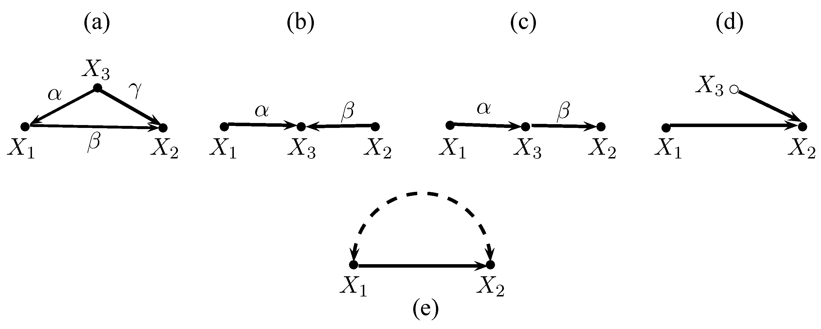
This section introduces causal graphs and the path-tracing rules that are used in this paper. Figure 1 shows five graphs. Solid nodes represent observed variables, hollow nodes represent unobserved variables, solid arrows indicate causal links, and curved dashed bi-directed arrows indicate covariances that arise from unspecified causes. Hence, all variables in Figure 1a–c are observed, is unobserved in Figure 1d, and causes in Figure 1e but the variables are also correlated because of other unmodeled causes.
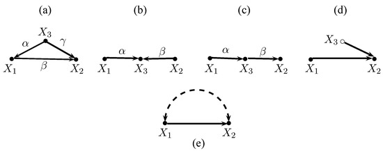
Figure 1.
Confounder (a), collider (b), mediator (c), unobserved cause (d), joint unobserved causes (e).
A path is a sequence of nodes connected by arrows. A path is d-connected if it does not traverse any collider.6 A variable is a collider on a path if two arrows are pointing into it. Thus, the paths and in Figure 1a are d-connected. The path in Figure 1b is not d-connected because is a collider that blocks the path.
A path between two variables and can be blocked or d-separated by a set of variables S in two ways. The path can be blocked by conditioning when the path contains a chain or a fork and the middle variable is in the conditioning set S. The path between and is also blocked when the path contains a collider and the collider (or any of its descendants) is not in the conditioning set S. As a consequence, two variables and are d-connected conditional on a set of variablesS if there is a collider-free path between them that does not traverse any member of S, or if there is a path between them where a collider is in the conditioning set S.
Two simple path-tracing rules (Pearl 2013) yield analytical expressions for covariances between variables in a graph.7 The resulting expressions for the covariances can be substituted into other formulas.
The first path-tracing rule applies to standardized variables (i.e., variables that have been normalized to have zero mean and unit variance). Let be the product of the path coefficients along a path i that d-connects two standardized variables A and B, say. Path coefficients can either be structural coefficients or covariances. The first rule states that the covariance between A and B is the sum of the products of the path coefficients along all d-connected paths between A and B, i.e., .
The second path-tracing rule extends the first path-tracing rule to non-standardized variables. The product associated with a path i of non-standardized variables A and B must be multiplied by the variance of the variable from which path i originates. Double arrows serve as their own origin. Thus, when A and B are non-standardized variables, then .
It is instructive to use the path-tracing rules to derive the covariance between and conditional on in Figure 1a–c, because the results show how conditioning on a third variable may affect the covariance between the other two variables. Equation (1) expresses the covariance between and conditional on ,
in terms of the unconditional covariances. For convenience, let us assume that , , and are standardized multivariate normally distributed random variables.8 Thus, .
In Figure 1a conditioning uncovers the causal effect of on . Fixing blocks the path . Path-tracing yields , and . Plugging these expressions into (1) yields .
In Figure 1b the variables and are independent. Thus, , but conditioning on the common outcome creates dependence between and . Intuitively, information about one of the causes makes the other cause more or less likely, given that we know the outcome. Here, , , and (1) yields .
In Figure 1c the variable mediates the effect of on . The unconditional covariance is . Conditioning on breaks this link, and .
3. Effect Indicators
In empirical studies it is common that a model for the dependent variable contains one or more explanatory variables of interest and some additional control variables that should help to identify causal effects of the explanatory variables of interest. Here we are interested in the causal effect of a latent variable L. In this paper, I always denotes an indicator of the latent variable. In this section, I is an effect indicator. Later, in Section 4 and Section 5, the letter I will denote a background indicator that is affected by a background variable B.
Let us now consider a linear structural model
where Y is the dependent variable, L is a latent variable, X is a column vector of control variables, is a row vector of coefficients, and u is an error term. The coefficient measures the effect of L on Y.
If L were observable, OLS would provide a consistent estimate for if in the population there is no exact linear relationship between the regressors and the error u has mean zero and is uncorrelated with each of the regressors.9 However, here we cannot observe L.
A standard solution to this problem is to find an indicator I of the latent variable of the form
where the error e is assumed to be uncorrelated with L. Most latent variables have no natural scale. It is, therefore, common to set , so that the observable indicator and the latent variable have the same scale.
Rearranging (3) and plugging in for L in (2) yields
where = and .10 It is easy to show that the indicator I is correlated with the compound error and therefore endogenous. Thus, OLS is inconsistent.
Let us now turn to IV estimation of model (4). For simplicity, let us assume that the structural model (2) has only a single control variable X and that all variables are demeaned such that . Let Z be an instrument for the latent variable L. The IV estimator for in the auxiliary model (4) is (Bowden and Turkington 1984)
When Z is uncorrelated with X (i.e., ) then Equation (5) collapses to the simple IV estimator
that arises when model (4) is estimated without X.11
Figure 2 depicts five causal graphs where I is an effect indicator of the latent variable L. Figure 2a shows a case where the error e in I and the error u in the structural model (2) are uncorrelated. This is the standard assumption made in applied work. One path connects Z and Y via L, and one path runs from Z via L to I. Hence, and = . Moreover, because the only path between Z and X is blocked by Y. Thus, the simple IV estimator applies. Plugging the expressions for and into (6) yields
and hence by imposing = 1 in (3).12
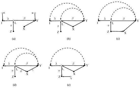
Figure 2.
Effect indicators.
Figure 2b relaxes the standard assumption of uncorrelated errors because the errors e and u are correlated. Furthermore, X is now a confounding variable, and the latent variable L in the structural model is endogenous because of neglected other joint causes of L and Y. These complications appear to be substantial, but they have no effect because L and I are colliders. In particular, . The simple IV estimator still applies, and there is no need to control for the confounding variable X.
Figure 2c shows a case where X is an outcome of Z and Y. Including X in the regression would now be harmful because the “back-door” path between Z and Y would be opened. Z is only a valid instrument for I without controlling for X. Path-tracing verifies that the simple IV estimator (6) works, but the IV estimator (5) that takes X into account does not.
In Figure 2d the latent variable affects the dependent variable directly and indirectly via the mediating variable X. Now, the IV estimator yields the direct effect of the latent variable L. The simple IV estimator yields , which is the total effect (i.e., the direct + the indirect effect) of L on Y. Hence, identification of the direct effect of the latent variable requires controlling for the mediating variable X.
In the former cases the instrument Z caused the latent variable L. Figure 2e shows a situation where the instrument Z is a second effect indicator of L. This apparently minor difference to the former cases has important consequences. First, the errors e and u may be correlated but the error v in Z must be uncorrelated with both errors. Second, the latent variable L must now be exogenous in the structural model (i.e., there must be no double arrows between L and Y). Third, one must control for all L – Y confounding variables. Then the ratio is identified. While conditioning L – Y confounders is necessary for identification, conditioning on L – Y mediators (such as the X variable in Figure 2d) is only necessary if one wants to disentangle direct and indirect effects of the latent variable and not to obtain the total effect. Thus, IV estimates of the effect of the latent variable that are based on two effect indicators require stronger assumptions than estimates where the instrument causes the latent variable.
4. Background Indicators
As already explained, background indicators are, in contrast to ordinary indicators, also systematically affected by variables that are not part of the original structural model. Background variables could be joint causes of the latent variable and the indicator, or they could be variables that mediate effects of the latent variable to the indicator.
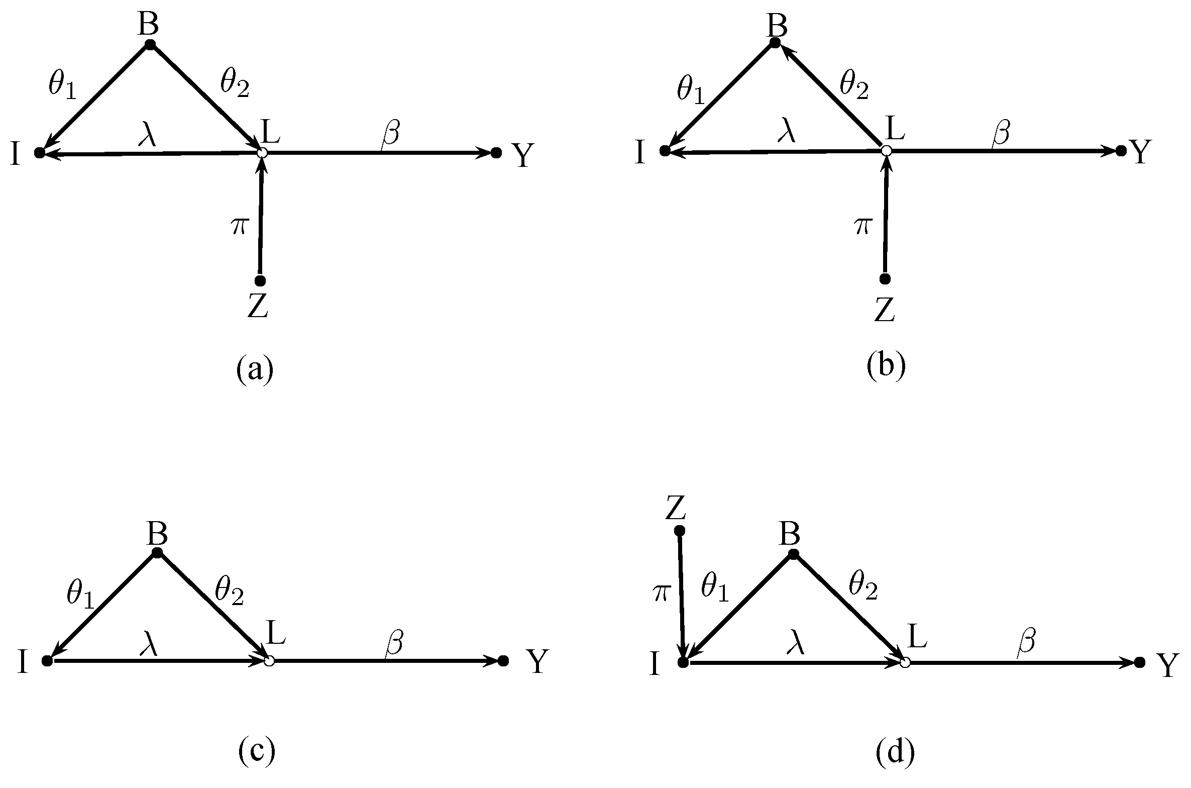
Figure 3 shows four cases with background indicators. For clarity, the graphs now abstract from error terms and additional control variables because these issues have already been discussed in the previous section.

Figure 3.
Background indicators.
Figure 3a,b describe cases that could occur in studies on the link between financial development and economic growth. In these examples Y is economic growth and L is financial development, which is the latent variable we are interested in. The variable I is a ratio of bank credit to GDP, B is a background variable such as international financial integration, and Z is an instrument for financial development. Empirical studies have for instance used the origin of the legal system of a country as an instrument for the development of its financial system (Levine et al. 2000).
In Figure 3a the background variable B causes the latent variable L and the indicator I. The covariance between Z and Y is , and the covariance between I and Z is . The resulting IV estimate is therefore
As can be seen, this estimate is not affected by the background indicator. The usual practice of setting may be more difficult to justify, however.
Figure 3b shows a situation where the latent variable affects the indicator directly and indirectly via the mediating background variable B. The covariances are now and . The IV estimate becomes
Thus, the presence of B biases the simple IV estimate. This bias can only be removed by controlling for B, as can be verified by computing the IV estimate using (5). Remarkably, in case (b) the background variable B must be included in the regression, even though B does not affect the dependent variable Y in the structural model.
Figure 3c,d shows two cases that could for example occur in studies about effects of uncertainty on economic activity. Here, Y is economic activity, L is the unobservable uncertainty, I is stock market volatility, a frequently used indicator of uncertainty, and B is a background variable.
Figure 3c,d depict a situation, as considered in Romer (1990), where a stock market crash or extreme stock market volatility becomes an additional source of uncertainty in an economy. Certain events B such as terrorist attacks, wars, or other bad events may raise uncertainty in the economy. Without a stock market there would be no further source of uncertainty. However, here a stock market exists, and the events B may also affect the uncertainty of stock traders about the future course of the economy. This uncertainty is reflected in the volatility of the stock market. Please note that the traders may sit anywhere (i.e., in large international financial institutions) and may not necessarily belong to the economy of interest. While people may not own stocks themselves, they interpret the stock market as a predictor of their future income, and they become nervous when they see extreme stock market volatility. Stock market volatility now becomes an additional source of uncertainty that amplifies the uncertainty in the economy even further.
As already mentioned, background indicators may easily get confused with ordinary effect indicators. Figure 3c depicts such a case. The background variable B captures exogenous events that simultaneously drive uncertainty L and stock market volatility I, but volatility amplifies uncertainty further. Variables that cause only the latent variable do not work as instruments here because such variables are necessarily uncorrelated with the indicator. Thus, one is tempted to use the exogenous variable B that is correlated with the indicator I as an instrument.
Using B mistakenly as an instrument for I yields and . The resulting IV estimate
is inconsistent. The estimate captures three distinct effects, namely the effect of I on Y, the effect of B on Y, and the strength of the effect of B on I. The estimate tends to the causal effect of I on Y when is small. When is close to zero the estimate blows up, because B becomes a weak instrument.
What does OLS yield when stock market volatility amplifies uncertainty? Since the OLS estimate
is also biased and inconsistent because the background variable B has been omitted. The second term in (11) reflects this bias.
Regressing Y on I and B removes the omitted variable bias in (11), but the resulting estimate is the causal effect of I on Y. In this example one would therefore estimate the causal effect of stock market volatility on output rather than the effect of uncertainty on output.
Let us now assume that . In this case, exogenous bad events affect the uncertainty of traders and the public to the same extent and stock market volatility fully amplifies uncertainty. Let us further assume that the effect of uncertainty on output is negative, as theory predicts.13 The IV estimate given in (10) becomes and the OLS estimate (11) is where r denotes the ratio of . Both quantities overestimate the magnitude of the (negative) effect of uncertainty, but OLS can get close to when r is small. In contrast, a weaker link (i.e., ) between B and I would inflate the IV estimate further.
Figure 3d shows a case where Z is indeed a valid instrument for stock market volatility I. Even if such an instrument could be found it would not solve the problem. Path-tracing yields and . The resulting IV estimate would capture the causal effect of stock market volatility on output rather than the effect of uncertainty on output.
5. Background Indicators as Instruments
We have seen that background indicators complicate the identification and estimation of effects of latent variables. In fact, identification becomes virtually impossible without an additional effect indicator for the latent variable when the background indicator causes the latent variable.
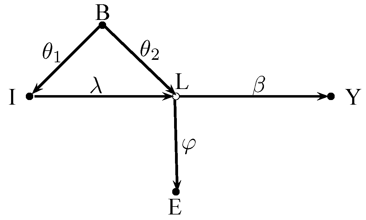
Figure 4 shows a case where we have two indicators for the latent variable L. The first indicator I is a background indicator. The second indicator E is an ordinary effect indicator. The graph abstracts again from error terms and control variables. All issues concerning the inclusion or exclusion of control variables discussed in Section 3 apply here as well.

Figure 4.
Background indicator as instrument.
The background indicator I can now be used as an instrument for E. The IV estimate is
and yields by setting . The background indicator I is also a valid instrument when the causal link goes from L to I or when B mediates the effect of L on I. There is no need to control for the background variable, but it must be kept in mind that one must control for all confounding or mediating variables that belong into the structural model when the background indicator is caused by the latent variable.
6. Simulations
The following simulation experiment considers the impact of uncertainty on aggregate consumption growth. The goal of the simulations is to illustrate some of the theoretical results. As mentioned earlier, economic theory predicts that uncertainty about future income reduces consumption, since the value of postponing consumption decisions increases with increasing uncertainty. In the simulations it is, therefore, assumed that higher uncertainty lowers aggregate consumption growth. Since uncertainty cannot be observed directly, consumption growth is regressed on the logarithm of stock market volatility, which is assumed to be an indicator of uncertainty. As is usual for macroeconomic series, the linear relationships between the variables are assumed to hold on the logarithmic scale. The estimated regression coefficient for the effect of uncertainty therefore measures the elasticity of consumption growth with respect to uncertainty in percentage terms.
6.1. Setup
The setup of the simulation experiment is very simple. A process
represents the flow of exogenous events that cause uncertainty. The parameter captures the average level of this process, and the parameter determines how fast the process moves towards its average. The random variable represents new events at time t. This variable is identically and independently distributed (iid) and follows a normal distribution with zero mean and variance , i.e., ∼ iid N(0,).
Logarithms are used to create an index of exogenous events that always has a positive numeric value. The basic idea is that adverse events receive larger numerical values than less adverse events. The autoregressive structure of Equation (13) reflects the idea that adverse events can trigger further adverse events.
plus unsystematic noise ∼ iid N(0, ) creates uncertainty of the amount
at time t.
The simulation experiment considers three different models. The first model () corresponds to Figure 2a.14 Here the logarithm of stock market volatility
is an ordinary effect indicator. The random noise in is iid N(0, ). Please note that stock market volatility itself is always positive by construction.
Consumption growth is generated as
with ∼ iid N(0, ). Thus, people reduce consumption when uncertainty exceeds its average level of and expand consumption when uncertainty is below average.
The second model () corresponds to Figure 3c. Uncertainty has now two sources that originate from the same background variable. The background variable affects uncertainty directly and indirectly via stock market volatility
Consumption growth is now given by
Thus, consumption growth slows down when the uncertainty that originates directly from adverse events is above the level and (or) when the observed level of stock market volatility is above .
The third model () combines () and (). People ignore lower levels of stock market volatility, but they get nervous when volatility is high. Thus, stock market volatility is a standard effect indicator as long as volatility remains below a critical level and consumption is determined by Equation (16). However, when volatility exceeds then volatility becomes a background indicator that causes uncertainty. In the latter case consumption follows Equation (18). Hence, in () consumption growth is generated as
where when and zero otherwise.
The above models are intended as very simple examples. Nevertheless, an attempt is made to obtain simulated data with realistic statistical properties. The parameters reported in Table 1 produce series that have statistical properties similar to US stock market volatility and US aggregate consumption growth.

Table 1.
Parameters
The upper part of Table 2 shows summary statistics for quarterly US consumption growth and quarterly stock market volatility for the period 1985q2–2011q4. The lower part of Table 2 reports the same statistics averaged across 1000 simulated volatility and consumption growth series obtained with models and .
Table 2.
Stock market volatility and consumption growth: statistics for US data and simulated data.
In the simulations the starting value in (13) is always ln. In each repetition 300 observations are generated. Then the first 100 observations are discarded to remove possible effects of the starting value. The remaining 200 observations are used in all further calculations.
Most statistics for the US data and the simulated data in Table 2 are quite similar. Only the minimum of simulated consumption growth tends to be somewhat too high, and the maximum of simulated stock market volatility tends to be somewhat too low compared to the US data. It must be remembered, however, that the US data cover the crisis of 2007–2009 where volatility skyrocketed, and consumption dropped dramatically.
The experiment considers three regressions of the type
In these regressions the estimated coefficient provides an estimate for the parameter = −0.5 of the negative effect of uncertainty on consumption growth. First, consumption growth is regressed on the true but unobservable amount of uncertainty (i.e., ). The results from this OLS regression provide a benchmark to evaluate the performance of the alternative estimators in terms of simulation variability. Next, consumption growth is regressed on the logarithm of stock market volatility (i.e., ) using OLS. Finally, the same equation is estimated with two stage least squares (2SLS).
In the 2SLS regression the instrument for is a dummy variable that captures “important exogenous events” that cause uncertainty. This dummy variable is constructed as in Bloom (2009) and Baker and Bloom (2012). In the simulations when ln exceeds the 75% percentile of its empirical distribution, otherwise .
6.2. Results
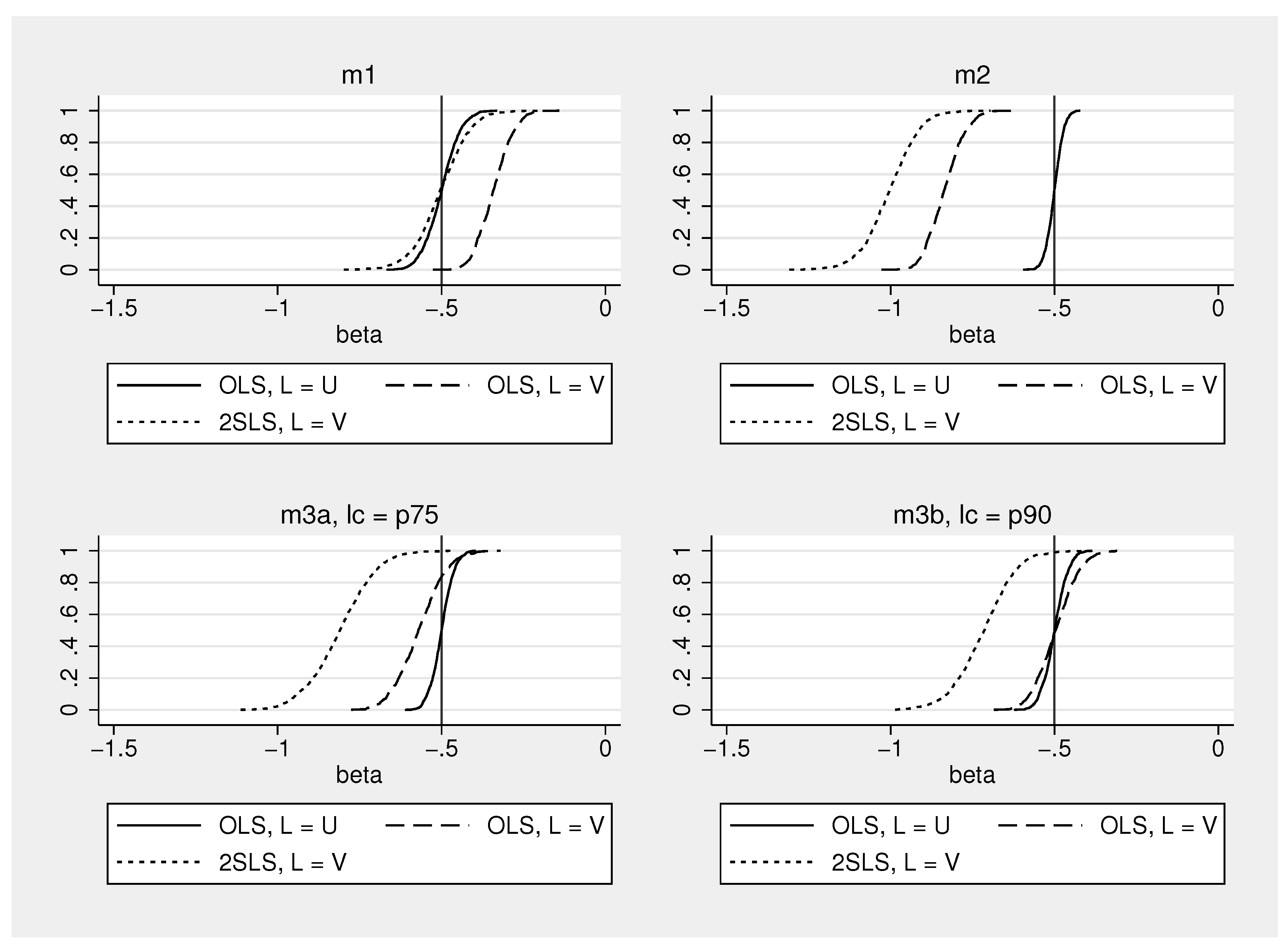
Figure 5 shows empirical distributions of the estimated coefficient in (20). The distributions are based on samples of 200 observations, generated as described above, and 1000 repetitions. Table 3 shows the medians of these distributions. Medians are reported because in finite samples the expectation of 2SLS estimates of in (20) based on a single instrument does not exist (Kinal 1980).
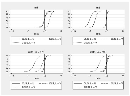
Figure 5.
Simulated distributions of OLS and 2SLS estimates of the effect of uncertainty on consumption.
Table 3.
Medians of estimated coefficients for simulated models.
The upper left graph in Figure 5 shows the distributions for from model . OLS is inconsistent as to be expected, and the estimates are biased towards zero when stock market volatility is substituted for uncertainty. 2SLS is consistent, but the estimates are more dispersed than in the OLS regression where consumption is regressed on the true amount of uncertainty.
The results for model where is a background indicator are displayed in the upper right half of Figure 5. Now, OLS and 2SLS clearly overestimate the negative effect of uncertainty on consumption when is used as an indicator. The median of the estimates is about −0.8 for OLS and −1 for 2SLS (see Table 3), which is in line with the theoretical results in Equations (11) and (10).
The lower part of Figure 5 shows results for two versions of model . In stock market volatility becomes an additional determinant of uncertainty when volatility exceeds the 75% percentile. Thus, 25% of the observations are determined by model and 75% are determined by model . As can be seen, OLS and 2SLS again overestimate the negative effect of uncertainty, but OLS tends now to be much closer to the true value of −0.5 than 2SLS.
In model only 10% of the observations come from . The rest comes from model . The 2SLS estimates are again quite far away from the true value, but the estimates of OLS with stock market volatility and OLS with the true amount of uncertainty are now very similar. This happens because the OLS bias (compare columns two and three in Table 3) under and goes into different directions and nearly cancels out under this weighting of the models and . Other weightings of models and and other parameter settings may of course lead to different results. Overall, the simulations provide a simple example for a situation where IV approaches overestimate the negative impact of uncertainty on economic activity when stock market volatility is a background indicator that becomes in certain periods an additional cause of uncertainty.
7. Conclusions
Background indicators of latent variables have until now been neglected although they might easily be confused with ordinary effect indicators. This paper studied simple linear models to gain a conceptual understanding of background indicators.
The analysis showed that background indicators produce inconsistent estimates of effects of latent variables in empirically relevant cases. In the simulation experiment, for instance, the estimated effects of uncertainty are too large when stock market volatility is a background indicator of uncertainty. Background indicators may be useful instruments, but they should not replace latent variables in a structural model. The results also suggest that the choice of indicators should, just like the choice credibility of instruments, be guided by theoretical considerations and careful judgment.
Future work could extend the analysis to nonlinear models. Analytical results are then of course more difficult to obtain. Another possible extension would be to investigate the usefulness of causal search algorithms for identifying background indicators. These issues are, however, beyond the scope of this paper and are left for future research.
Funding
This research received no external funding.
Acknowledgments
I would like to thank the three anonymous referees for their helpful comments and suggestions.
Conflicts of Interest
The author declares no conflict of interest.
References
- Abel, Andrew B., and Janice C. Eberly. 1996. Optimal Investment with Costly Reversibility. Review of Economic Studies 63: 581–93. [Google Scholar] [CrossRef]
- Baker, Scott R., and Nicholos Bloom. 2012 Does uncertainty reduce growth? Using disasters as natural experiments. unpublished manuscript.
- Bernanke, Ben S. 1983. Irreversibility, Uncertainty, and Cyclical Investment. The Quarterly Journal of Economics 98: 85–106. [Google Scholar] [CrossRef]
- Bertola, Guiseppe, and Ricardo J. Caballero. 1994. Irreversibility and Aggregate Investment. Review of Economic Studies 61: 223–46. [Google Scholar] [CrossRef]
- Bloom, Nicholas. 2009. The Impact of Uncertainty Shocks. Econometrica 77: 623–85. [Google Scholar]
- Bollen, Kenneth A. 1989. Structural Equations with Latent Variables. Hoboken: Wiley. [Google Scholar]
- Bowden, Roger J., and Turkington Darrell A. 1984. Instrumental Variables. Cambridge: Cambridge University Press, p. viii, 227. [Google Scholar]
- Brito, Carlos, and Judea Pearl. 2002. Generalized Instrumental Variables. Paper presented at Eighteenth Conference on Uncertainty in Artificial Intelligence, UAI’02, Edmonton, AL, Canada, August 1–4. [Google Scholar]
- Carruth, Alan, Andy Dickerson, and Andrew Henley. 2000. What Do We Know about Investment under Uncertainty? Journal of Economic Surveys 14: 119–53. [Google Scholar] [CrossRef]
- Chen, Bryant, and Judea Pearl. 2014. Graphical Tools for Linear Structural Equation Modeling. Technical Report, r-432. California: University of California. [Google Scholar]
- Cramér, Harald. 1946. Mathematical Methods of Statistics. Princeton: Princeton University Press, p. xvi, 575. [Google Scholar]
- Dixit, Avinash K., and Robert S. Pindyck. 1994. Investment under Uncertainty. Princeton: Princeton University Press. [Google Scholar]
- Farmer, Roger E.A. 2015. The Stock Market Crash Really Did Cause the Great Recession. Oxford Bulletin of Economics and Statistics 77: 617–633. [Google Scholar] [CrossRef]
- Giannetti, Mariassunta, and Steven Ongena. 2009. Financial Integration and Firm Performance: Evidence from Foreign Bank Entry in Emerging Markets. Review of Finance 13: 181–223. [Google Scholar] [CrossRef]
- Goldberger, Arthur S. 1972. Structural Equation Methods in the Social Sciences. Econometrica 40: 979–1001. [Google Scholar] [CrossRef]
- Hoover, Kevin D. 2001. Causality in Macroeconomics. Cambridge: Cambridge University Press. [Google Scholar]
- Kinal, Terrence W. 1980. The Existence of Moments of k-Class Estimators. Econometrica 48: 241–49. [Google Scholar] [CrossRef]
- Kuroki, Manabu, and Judea Pearl. 2014. Measurement bias and effect restoration in causal inference. Biometrika 101: 423–37. [Google Scholar] [CrossRef]
- Leduc, Sylvain, and Zheng Lui. 2013. Uncertainty Shocks Are Aggregate Demand Shocks. Working Paper 2012-10. San Francisco: Federal Reserve Bank of San Francisco. [Google Scholar]
- Levine, Ross, Norman Loayza, and Thorsten Beck. 2000. Financial intermediation and growth: Causality and causes. Journal of Monetary Economics 46: 31–77. [Google Scholar] [CrossRef]
- Levine, Ross. 2005. Finance and Growth: Theory and Evidence. In Handbook of Economic Growth. Edited by P. Aghion and N.D. Stephen. Amsterdam: Elsevier B. V., vol. 1A, pp. 885–934. [Google Scholar]
- McDonald, Robert, and Daniel R. Siegel. 1986. The Value of Waiting to Invest. Quarterly Journal of Economics 101: 707–27. [Google Scholar] [CrossRef]
- Morgan, S.L., and Christopher Winship. 2007. Counterfactuals and Causal Inference: Methods and Principles for Social Research. Cambridge: Cambridge University Press. [Google Scholar]
- Pearl, Judea. 2009. Causality: Models, Reasoning and Inference, 2nd ed. Cambridge: Cambridge University Press. [Google Scholar]
- Pearl, Judea. 2013. Linear Models: A useful “Microscope” for Causal Analysis. Journal of Causal Inference 1: 155–70. [Google Scholar] [CrossRef]
- Ramey, Garey, and Valerie A. Ramey. 1995. Cross-Country Evidence on the Link between Volatility and Growth. American Economic Review 85: 1138–51. [Google Scholar]
- Romer, Christina D. 1990. The Great Crash and the Onset of the Great Depression. The Quarterly Journal of Economics 105: 597–624. [Google Scholar] [CrossRef]
- Spirtes, Peter, Christopher Meek, and Thomas Richardson. 1995. Causal Inference in the Presence of Latent Variables and Selection Bias. Paper presented at Eleventh Conference on Uncertainty in Artificial Intelligence, UAI’95, Montréal, QC, Canada, August 18–20. [Google Scholar]
- Spirtes, Peter, Clark Glymour, and Richard Scheines. 2000. Causation, Prediction, and Search, 2nd ed. Cambridge: The MIT Press. [Google Scholar]
- Stanghellini, Elena, and Nanny Wermuth. 2005. On the identification of path analysis models with one hidden variable. Biometrika 92: 337–50. [Google Scholar] [CrossRef]
- Vera, F. 2000. Three Essays on the Variable Selection Problem. Ph.D. dissertation, Texas A & M University, College Station, Texas, USA. [Google Scholar]
- Wooldridge, Jeffrey M. 2010. Econometric Analysis of Cross Section and Panel Data, 2nd ed. Cambridge: The MIT Press. [Google Scholar]
- Wright, Sewall. 1921. Correlation and Causation. Journal of Agricultural Research 20: 557–585. [Google Scholar]
| 1. | This paper follows Wooldridge (2010) and distinguishes between indicators and proxy variables. A proxy variable is usually a variable that helps to explain the latent variable whereas an indicator is usually a measurement of an effect of the latent variable. See Wooldridge (2010) chp. 4 and chp. 5 for further details. |
| 2. | See, Levine (2005) for a survey of the literature on finance and growth. |
| 3. | Ramey and Ramey (1995), Carruth et al. (2000), Bloom (2009), Baker and Bloom (2012), Leduc and Lui (2013), among others. |
| 4. | See, Hoover (2001) for one of the rare applications of causal graphs in economics. Other important early work includes Spirtes et al. (1995), Spirtes et al. (2000), and Vera (2000). |
| 5. | Stanghellini and Wermuth (2005) and Kuroki and Pearl (2014) also analyze identification in linear models when a latent variable is present. However, in contrast to this paper, these authors focus on identification of effects of observed variables. |
| 6. | The d stands for dependence. |
| 7. | Both rules follow from covariance mathematics and date back to Wright (1921). See, Goldberger (1972), and Bollen (1989) for further details. |
| 8. | Under the multivariate normality assumption the conditional covariance between and does not change for different values of . See, Cramér (1946). Under more general assumptions this covariance may depend on the specific values of . |
| 9. | See, Wooldridge (2010) chp. 4 for further details. |
| 10. | |
| 11. | Equation (5) results from the standard instrumental variable estimator when the linear model has two explanatory variables I and X, and when Z is the instrument for I and X is the instrument for itself. This estimator is the same as the corresponding conditional instrumental variable estimator of Brito and Pearl (2002). |
| 12. | Throughout the paper variances are understood to be population variances to which the corresponding estimated variances eventually converge in large samples. |
| 13. | See Bernanke (1983); McDonald and Siegel (1986); Dixit and Pindyck (1994); Bertola and Caballero (1994), and Abel and Eberly (1996) among others. |
| 14. | With and in Figure 2a. |

© 2019 by the author. Licensee MDPI, Basel, Switzerland. This article is an open access article distributed under the terms and conditions of the Creative Commons Attribution (CC BY) license (http://creativecommons.org/licenses/by/4.0/).