Abstract
Hermes is a Single-Input Single-Output (SISO) underwater acoustic modem that achieves very high-bit rate digital communications in ports and shallow waters. Here, the authors study the capability of Hermes to support Multiple-Input-Multiple-Output (MIMO) technology. A least-square channel estimation algorithm is used to evaluate multiple MIMO channel impulse responses at the receiver end. A deconvolution routine is used to separate the messages coming from different sources. This paper covers the performance of both the channel estimation and the MIMO deconvolution processes using either simulated data or field data. The MIMO equalization performance is measured by comparing three relative root mean-squared errors (RMSE), obtained by calculations between the source signal (a pseudo-noise sequence) and the corresponding received MIMO signal at various stages of the deconvolution process; prior to any interference removal, at the output of the Linear Equalization (LE) process and at the output of an interference cancellation process with complete a priori knowledge of the transmitted signal. Using the simulated data, the RMSE using LE is −20.5 dB (where 0 dB corresponds to 100% of relative error) while the lower bound value is −33.4 dB. Using experimental data, the LE performance is −3.3 dB and the lower bound RMSE value is −27 dB.
1. Introduction
Hermes is a broadband, high-frequency (262 kHz–375 kHz) Under Water Acoustic (UWA) modem designed for very high-bit rate digital communications in ports and shallow waters. In its current form, this modem supports only a single source and a single receiver [1,2,3]. In this paper, the authors apply Multiple-Input-Multiple-Output (MIMO) technology to Hermes, so that multiple sources and receivers distributed over an area can be used simultaneously. While the channel estimation algorithm (previously presented in [4]) and the MIMO deconvolution technique presented here are well known in the literature [5,6,7], the important contribution of the paper is to present a performance analysis when applied to high-frequency MIMO data, either simulated or experimental.
MIMO UWA communication is achieved by modifying the signaling of the FAU Hermes uplink message. The limited bandwidth, reliability and flexibility observed with UWA communication systems can be partly resolved by the use of MIMO techniques [5,8,9,10,11,12,13]. Indeed, the capability to send different messages via each source can significantly increase the overall data rate of the UWA communication system. In addition, the coverage area of the UWA modem can be significantly increased. However, MIMO communication systems cannot guarantee perfect communications, as signal fading; Doppler spread and ambient noise impair the overall performance of any UWA modem [14,15,16].
The proper retrieval of MIMO messages requires both an accurate estimation of the acoustic channels and an effective channel equalization algorithm. The least-square (LS) channel estimation algorithm was presented in a previous paper [4]. Here, the authors focus on channel deconvolution (MIMO equalization), which is critical to properly separate the messages coming from multiple sources (this is also called co-antenna interference removal) and to remove inter-symbol interference due to acoustic multipath. The deconvolution is implemented as a Minimum Mean Square Error (MMSE) equalizer. The theoretical limit of the deconvolution process is computed with an Interference Cancellation Linear Equalizer (ICLE), which removes the co-antenna interference by using a priori information on the transmitted sequence. Finally, the system performance is studied using simulated data, experimental data and the upper performance bound.
2. System Model
2.1. Source Signals
The messages sent through the acoustic channels are obtained by modifying the signaling of Hermes [1,2,3]. In this paper, i represents the source index. The proposed message is composed of the source-dependent MIMO sequence si,h (t) followed after a predefined time delay τmsg with the traditional Hermes message si,msg(t), such that:
 si,h(t) consists of perfectly known pseudo noise (PN) sequences of length τ = 218.5 ms, up-sampled from the symbol frequency Fsym to the sampling frequency and pulse-shaped using a raised-cosine filter. Figure 1 shows an example of source signal. Given a carrier frequency F0 and a signal level SL, the transmitted signal is
 where
where
 here, β is the roll-off coefficient and Tsym is the symbol period.
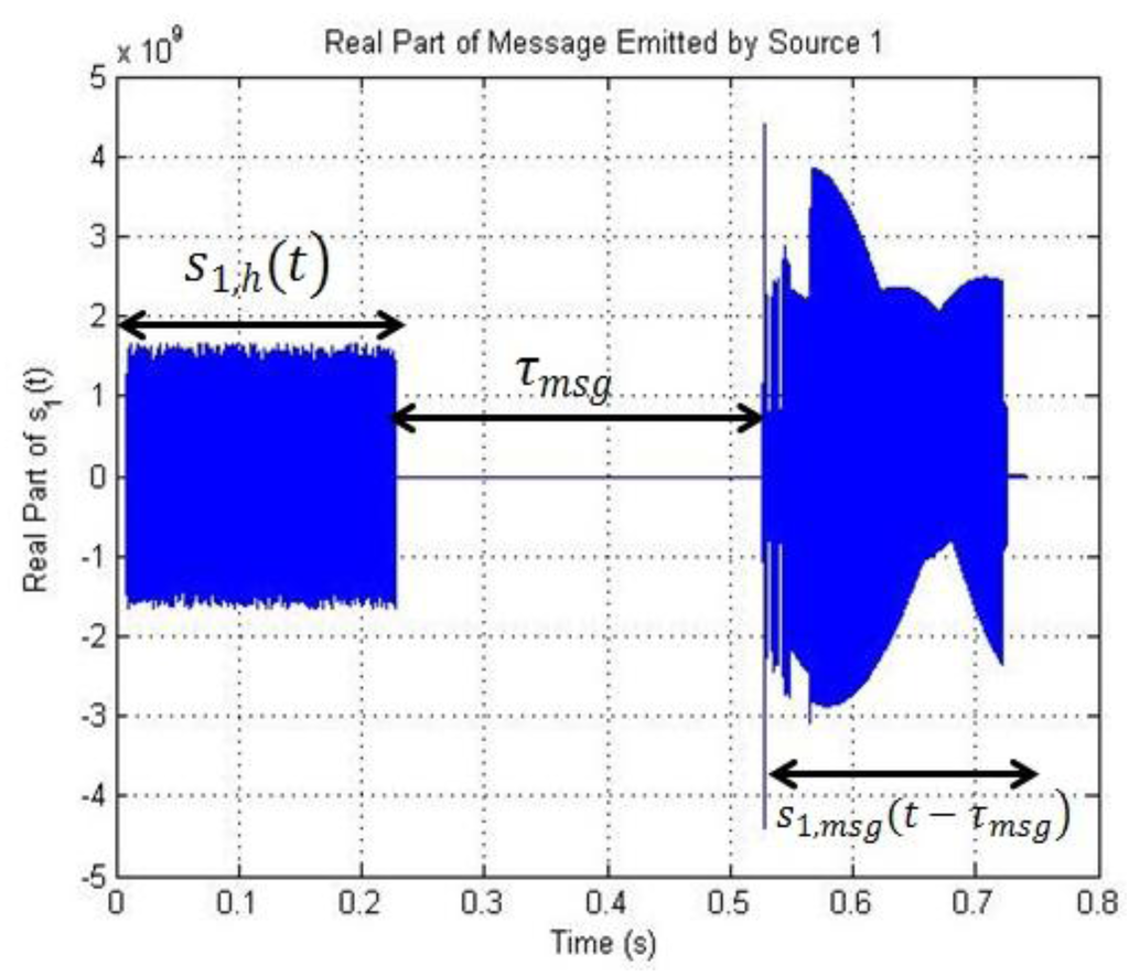
Figure 1.
Real part of source message 1.
In this paper, we assume that the message following the MIMO sequence does not change with the source. The MIMO sequences (one per source) have a very low cross-correlation to their auto-correlation peak ratio. We observed that the peak ratio is approximately 40 (which is equivalent to 16 dB).
2.2. Received Signals
In this section, we present the operations carried out at the receiver end. We first focus on the channel estimation algorithm, followed by the equalization. The derivations are provided in the discrete time domain, where k stands for the time index and l the delay index.
2.2.1. Channel Estimation
This process is performed over the duration of Nwin time windows, of time index twin and length Lwin. The received samples  at receiver j can be written in matrix form [4,17]:
 where
where  represents the augmented source signal array at the j th receiver.
  represents the augmented channel impulse response array.
  represents the noise array.
at receiver j can be written in matrix form [4,17]:
represents the augmented source signal array at the j th receiver. represents the augmented channel impulse response array. represents the noise array.As depicted in Figure 2, k0(twin) denotes the beginning of the time window. Lij is the length of the channel impulse response between transmitter i and receiver j, and  . Finally, Tj is the sum of the channel lengths over the total number of transmitters Nt, so that
  .
.
. Finally, Tj is the sum of the channel lengths over the total number of transmitters Nt, so that .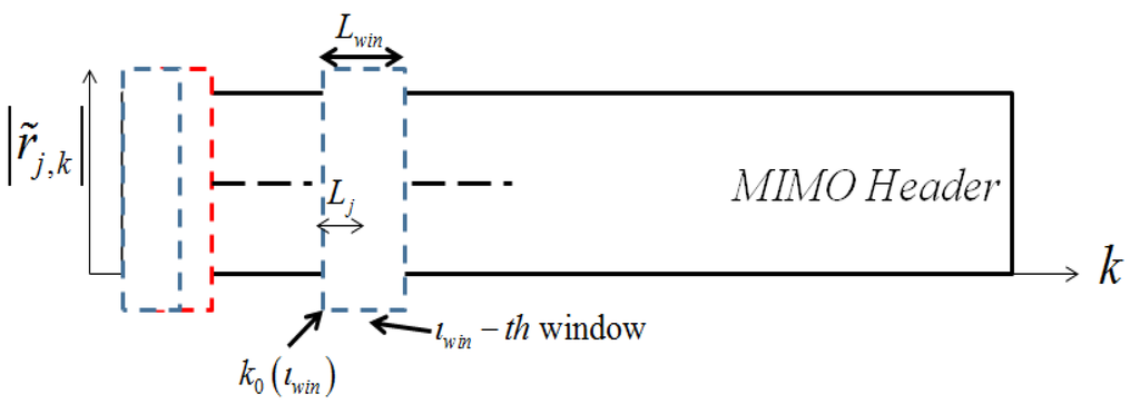
Figure 2.
Definition of the parameters of the time-window used to perform the channel estimation at receiver j.
In the continuous time domain, the quantity Tj is noted TL (this term is also used in the results section). The index j must be dropped, as the tunable parameter TL is assumed identical across every receiver. We study the influence of this parameter on channel estimation and deconvolution in the results section. The channel estimation is performed through minimization of the following quantity [18],

This leads to the LS estimation of  for every time window index twin,
 where ( )H represents the Hermitian operator. This operation requires a Tj × Tj matrix inversion.
for every time window index twin,
2.2.2. MIMO Deconvolution
The MIMO deconvolution process presented in this paper compensates for co-channel and inter-symbol interferences using the LS channel estimation obtained in Equation (6). The critical parameters identified in this performance study are: (1) the length of the channel estimate TL; (2) the length Tk of the pre-cursor and post-cursor of the linear equalization filter. We consider two equalization structures: conventional Linear Equalization (LE) and Interference Cancellation Linear Equalization (ICLE). ICLE provides a theoretical lower bound of the equalization process.
2.2.2.1. Minimum Mean Squared Error Linear Equalization
The process presented in this section consists of a feed-forward multi-channel linear filter optimized under MMSE criterion. Let L represent the maximum value of the sub-channel length Lij,

We define the matrices  and
and  as the received signal and noise over the total number of hydrophones:
 and
and

and as the received signal and noise over the total number of hydrophones:
Similarly, we define the transmitted signals  and channel impulse responses
  as:
as:


and channel impulse responses as:
Therefore, the received signal becomes

We now define κ1 and κ2 (Figure 3) as the pre-cursor and post-cursors of the linear equalization filter. In this case,  ,
,  and
and  are defined as


, and are defined as
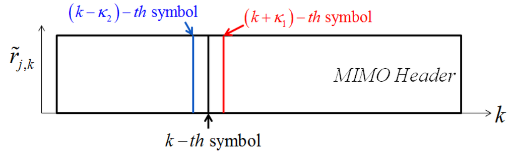
Figure 3.
Multiple-Input-Multiple-Output (MIMO) deconvolution process: pre-cursor and post-cursor definition.
In the results section, the influence of the pre-cursor and post-cursor is studied in the continuous time domain. In this paper, the length of these cursors is assumed to be the same and is represented by Tk. Next, we define the augmented matrix containing the matrices of channel impulse responses, denoted  ,
,
 so that
,
yk = Hxk + wk
The output of LE process can be expressed as:

In the sense of the MMSE criterion without any a priori on transmitted symbols, the optimum equalization filter is [5,18],
 where I is the identity matrix of size (1 + κ1 + κ2) Nr,
  is the variance of the noise and
  is the variance of the original sequence SI,K.
  denotes a column vector of size (L + κ1 + κ2) Nt with 1 at index i and 0 at other positions.
  is the estimates of augmented channel matrix H or time window index twin Here, the estimated signal
  depends on length of the time window, which in turns depends on the measured channel response. If Nwin = 1, the channel is stationary over a message duration and

is the variance of the noise and is the variance of the original sequence SI,K. denotes a column vector of size (L + κ1 + κ2) Nt with 1 at index i and 0 at other positions. is the estimates of augmented channel matrix H or time window index twin Here, the estimated signal depends on length of the time window, which in turns depends on the measured channel response. If Nwin = 1, the channel is stationary over a message duration and
However, if Nwin ≥ 1,  becomes a function of twin. In this case, the equalized signal for each sliding window is cropped and forms a section of the equalized output ,

becomes a function of twin. In this case, the equalized signal for each sliding window is cropped and forms a section of the equalized output ,
The variables twin, Lwin and OR represent the time window index, length and overlapping rate, respectively.
2.2.2.2. MMSE Interference Cancellation Linear Equalizer
The ICLE has been developed to evaluate the best possible performance of the deconvolution process by assuming that the source signal is perfectly known. The output of the ICLE may be expressed as follows [6,7,19],
 yk is defined in Equation (17). pi,k and qi,k respectively stand for the feed-forward and feed-back filters. vi,k is defined as
 where,
 KICLE is the discrete delay index induced by the equalizer, such that 0 ≤ KICLE ≤ NICLE + L − 2, where NICLE represents the discrete ICLE length. Under MMSE optimization, the feed-forward and feed-back equalization vectors become equal to [7]:
 where
where
 and
and
 ek is a null column vector, with the exception of element Nt(k − 1) + i equal to 1. represents the noise variance. The ICLE estimate
  depend on the number of time windows used to perform the channel estimation, thus Equations (23)–(25) also apply to .
represents the noise variance. The ICLE estimate depend on the number of time windows used to perform the channel estimation, thus Equations (23)–(25) also apply to .3. Simulated and Experimental Results
The results, in terms of MIMO deconvolution, are presented in this section. The simulation parameters and the metrics are first presented, followed with a description of the experimental setup. The simulated results are analyzed: in this case, the channel is stationary over the duration of the message. Finally, a set of field data is analyzed, where time variations of the channel are observed.
3.1. Experimental Setup
A series of experiments was carried out in the Florida Atlantic University Seatech marina (Figure 4). While the experimental setup presented here uses two sources and three receivers, this paper presents only the results obtained with two receivers. Table 1 provides a summary of the data collection. A first set of data was acquired on 27 September 2011. A second series of experiments took place on 31 August 2011. The two sources were alternatively placed at the two locations labeled “Pos1” and “Pos7” in Figure 4. Two splash proof boxes were built to prevent any damage to the modem sources and were installed on kayaks. Each box contained a set of Hermes source electronics, an ITC-1089 source transducer and a battery pack. The source level was 179 dB ref. 1 μPa at 1 m. The receivers used to carry out these missions were deployed off a small research vessel. The experimental ranges are given in Table 2. The signals presented in this paper were acquired at a maximum range of 27 m. This short range is mostly due to the high sound absorption loss (100 dB/km at 20 °C and at 300 kHz [20]).
Since the equipment did not have the ability to perform real-time MIMO communication, each source was used individually and the MIMO messages were constructed off-line. The signal-to-noise ratio SNRj was calculated at each receiver j. The value of SNRj, averaged across every messages within a mission, is shown in Table 3. The observed SNR value varied between 27.1 dB and 34.3 dB from mission to mission. These variations are mostly due to the time varying characteristics of the channel, which dramatically impacts the average power of the received signals.
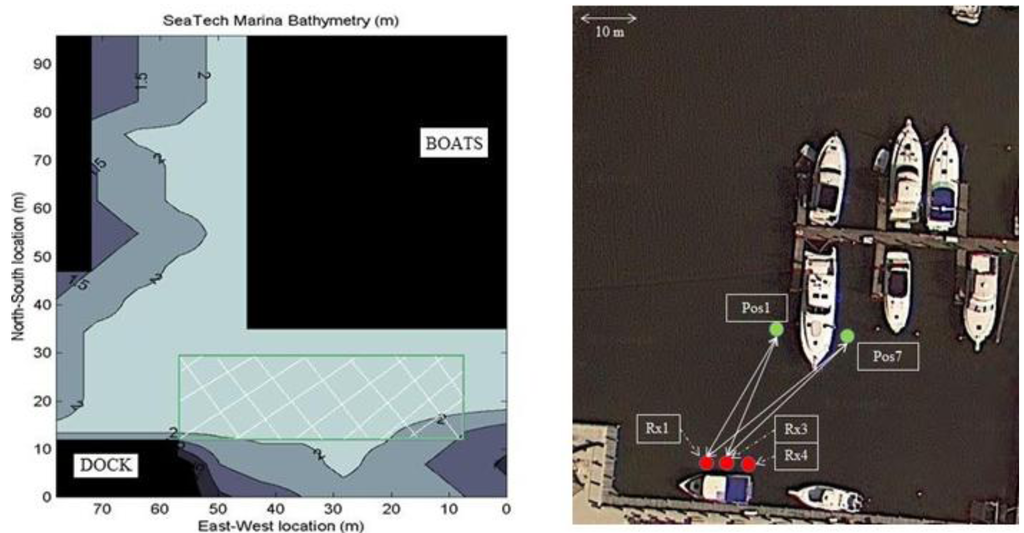
Figure 4.
Experimental setup.

Table 1.
Summary of data collected.
| Mission Number and Date | Source 1 Position | Source 2 Position | Receiver 1 Position | Receiver 2 Position | Number of Messages Retained |
|---|---|---|---|---|---|
| 1-07/27/2011 | Pos1 | Pos7 | Rx1 | Rx3 | 50 |
| 2-07/27/2011 | Pos7 | Pos1 | Rx1 | Rx3 | 50 |
| 3-08/29/2011 | Pos7 | Pos1 | Rx1 | Rx3 | 100 |
| 4-08/29/2011 | Pos1 | Pos7 | Rx1 | Rx3 | 100 |
Table 2.
Experimental ranges.
| Distance on Figure 4 | Distance (m) |
|---|---|
| Rx1-Pos1 | 24 |
| Rx1-Pos7 | 27 |
| Rx3-Pos1 | 23.3 |
| Rx3-Pos7 | 25.8 |
| Pos1-Pos7 | 6.15 |
| Rx1-Rx3 | 2.68 |
Table 3.
Signal-to-noise ratio per mission and per receiver.
| Mission Number and Date | SNR1(dB) | SNR2(dB) |
|---|---|---|
| 1-07/27/2011 | 27.1 | 27.3 |
| 2-07/27/2011 | 28.8 | 27.8 |
| 3-08/29/2011 | 30.9 | 34.3 |
| 4-08/29/2011 | 29.2 | 33.2 |
3.2. Simulation Parameters
The channel model, presented in detail in [4,17], combines a deterministic model (to determine the average echo intensities) [15,16] and a stochastic Rician model (to add some random fluctuation to every echo intensity) [4]. Sources and receivers’ separation and depth match the experimental setup presented in Section 3.1.
The simulation parameters (Table 4) are tuned to match the experimental data sets as closely as possible. Doppler shift and Doppler spread have been derived from the field data. The time window used to perform the channel estimation covers the duration of the MIMO sequence and the dead-time interval. Hence, the channel is assumed to be time-invariant over the transmission of a message. The coherence time of the channel therefore corresponds to the total length of the transmitted message: each new transmission would lead to a different channel to estimate.
For every transmitted message, we also adjust the time delay τ0 between the signals measured at every receiver. In this paper, we only consider full overlap between received messages. The results for partial overlap are presented in [17]. The channel model considered here includes both the specular reflection from the sea bottom and scattering from the sea surface and bottom.
Table 4.
Simulation parameters. Some of the simulation parameters are not formally used in the equations listed in this paper. The parameter name is followed with references [4,17], where the equations using these parameters are provided.
| Name | Symbol | Value (units) | Name | Symbol | Value (units) |
|---|---|---|---|---|---|
| Sources Depth [4,17] | DSi | 1 m | Source Level | SL | 179 dB re 1 µPa @ 1 m |
| Receivers Depth [4,17] | DRj | 1.5 m | Noise Level | NL | 83.7 dB re 1 µPa |
| Water Depth [4,17] | DW | 3 m | Sampling Frequency | FS | 150 kHz in base band 750 kHz in pass band |
| Water Sound Speed [4,17] | C | 1,500 m/s | Symbol Rate | Dsym | 75 kHz |
| Water Density [4,17] | ρ | 1,023 kg/m3 | Carrier Frequency | f0 | 0 kHz in base band 300 kHz in pass band |
| Sandy Sediment Sound Speed [4,17] | Cb | 1,800 m/s | MIMO Sequence Duration | τh | 218.5 ms |
| Sandy Sediment Density [4,17] | ρb | 1,800 kg/m3 | Dead-Time Duration | τmsg | 300 ms |
| Sea Bottom Loss [4,17] | LSB | 5 dB | Correlation Threshold Parameter | Kthr | 20 |
| Beginning of Time Window [4,17] | k0 | 0 | Time Window Length | τwin | 518.5 ms |
| Number of Transmitters [4,17] | Nt | 2 | Number of Receivers | Nr | 2 |
| Distance Source 1 Receiver 1 [4,17] | R11 | 23.3 m | Distance Source 1 Receiver 2 [4,17] | R12 | 24 m |
| Distance Source 2 Receiver 1 [4,17] | R21 | 25.8 m | Distance Source 2 Receiver 2 [4,17] | R22 | 27 m |
3.3. Performance Metrics
First, we present the performance of the channel estimation process. This performance is measured using the RMSE between the received MIMO header and the MIMO header convolved with the estimated channel, averaged across every message m and every receiver j [17]:

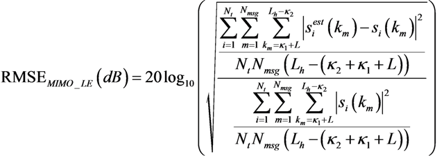
The MIMO LE performance is measured using the relative RMSE between the deconvolved MIMO header and the original sequence. This metric indicates the accuracy of the co-antenna and inter-symbol interference removal process. In this case, the RMSE is given by [17]:
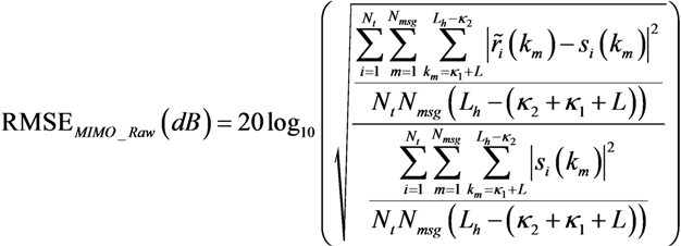
In order to evaluate the impact of the linear equalization on the received signals, RMSEMIMO_LE is compared to another relative RMSE between emitted and raw received signals. This second metric is calculated by comparing the received MIMO header signal (prior to any interference removal) and the corresponding source signal [17]:
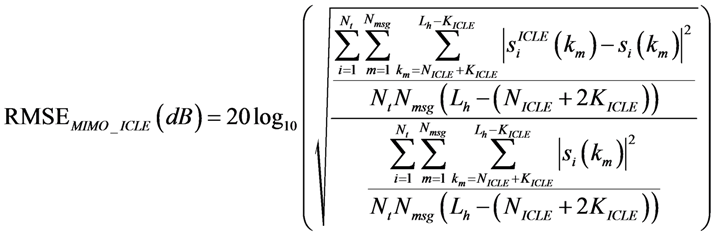
The performance estimated with the ICLE represents the theoretical performance limit of the MIMO LE. The relative RMSE between emitted MIMO sequences and the output of the ICLE is [17]:
3.4. MIMO Channel Estimation Results
Table 5 shows the values of RMSECE as a function of TL for both experimental and simulated data. The maximum value of TL is 5.33 ms, as higher values of TL lead to singularities and does not produce accurate results. As a reminder, RMSECE measures the error between the received signals and the emitted sequences convolved with the estimated channels. RMSECE is averaged across every receiver, so that the results presented in Table 5 translate the accuracy of the channel estimation across every sub-channel.
Table 5.
Relative root mean-squared errors (RMSECE) as a function of TL.
| TL(ms) | Simulated RMSECE (dB) | Experimental RMSECE (dB) |
|---|---|---|
| 0.667 | −9.5 | −0.4 |
| 1.333 | −12.5 | −0.9 |
| 2.0 | −18.8 | −4.1 |
| 2.667 | −34.7 | −4.9 |
| 3.333 | −34.7 | −6.2 |
| 4.0 | −34.7 | −9.1 |
| 4.667 | −34.8 | −11.4 |
| 5.33 | −34.8 | −25.7 |
In both experimental and simulation cases, as TL increases, the accuracy of the channel estimation improves. However, while RMSE CE reaches a sweet-spot at TL = 2.667 ms using simulated data (  ), the experimental results on RMSECE differ. Indeed, the minimum RMSECE is obtained for TL = 5.33 ms (RMSECE = −25.7 dB) as shown in Table 5 and Figure 5. If, as explained earlier on, values higher than TL = 5.33 ms cannot be considered, the minimum value of RMSECE using experimental data is of the same order of magnitude as RMSECE in the simulation framework. The channel estimation can therefore be considered as very accurate.
), the experimental results on RMSECE differ. Indeed, the minimum RMSECE is obtained for TL = 5.33 ms (RMSECE = −25.7 dB) as shown in Table 5 and Figure 5. If, as explained earlier on, values higher than TL = 5.33 ms cannot be considered, the minimum value of RMSECE using experimental data is of the same order of magnitude as RMSECE in the simulation framework. The channel estimation can therefore be considered as very accurate. Figure 5 displays the influence of TL on the channel estimation accuracy in the specific case of mission 4. Figure 6 shows that RMSECE drops and the confidence interval [−σCE;σCE] gets narrower as TL increases.
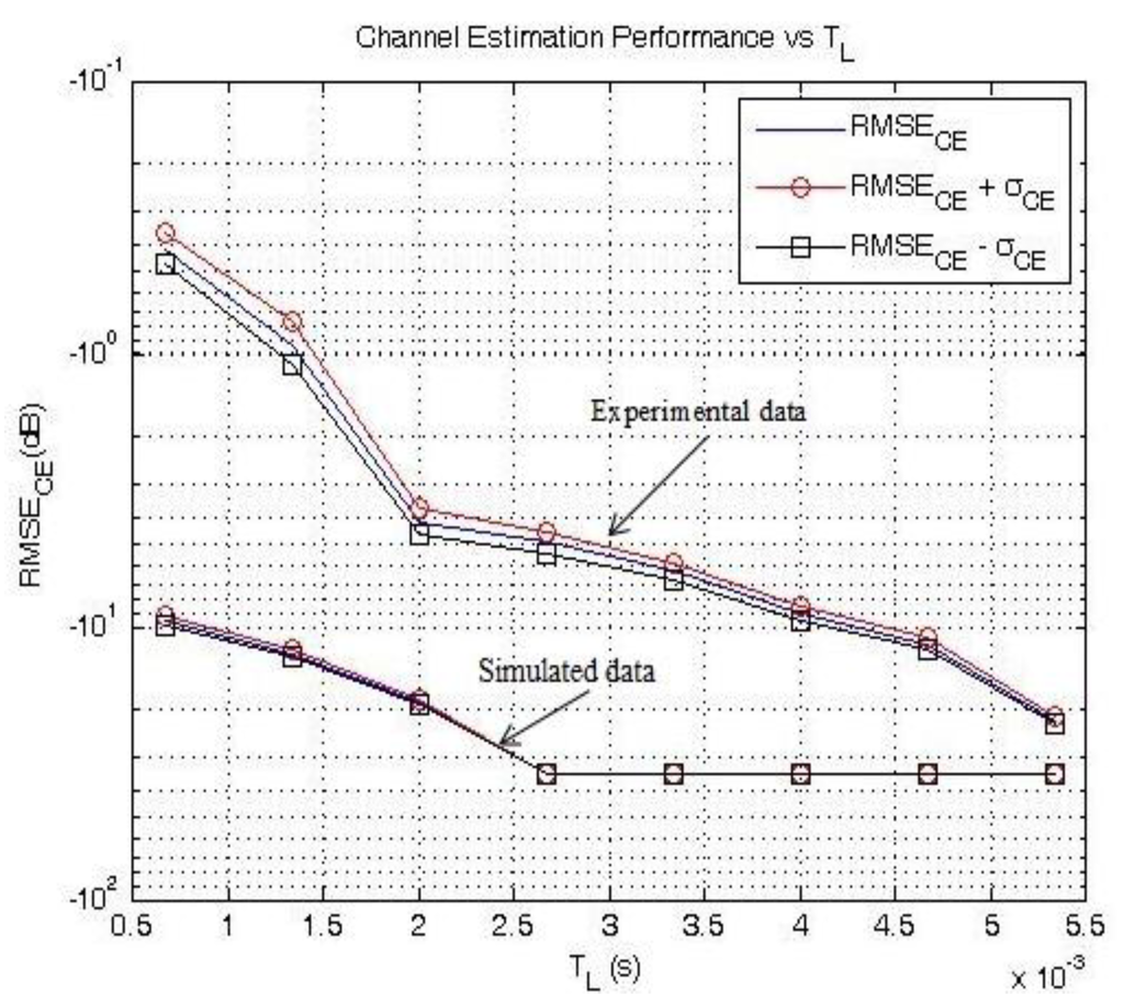
Figure 5.
RMSECE and RMSECE ± σCE as a function of TL.
The SNR is simply computed as the ratio of the received MIMO header power over the ambient noise power. It is also interesting to look at the impact of the SNR on the channel estimation performance for every receiver and every mission carried out. The best possible estimation of the channel impulse response is obtained when RMSECE at the output of the channel estimator (Equation (28)) is the inverse of the SNR. In this ideal case, the relationship can be rewritten in dB,
where the SNR is simply computed as the ratio of the received MIMO header power over the ambient noise power.
SNR(dB) = −RMSECE (dB)
In the more realistic case of imperfect channel estimation, Equation (4) should account for the residual error in estimating the channel impulse response at receiver j. This error can be modeled as an additive noise  , such that:

, such that:
We can verify the validity of such an approximation by comparing the SNR as shown in Table 2 and the RMSECE(dB) (Equation (28)) obtained for each of the corresponding four missions and for each receiver. In theory, when the best possible estimation of the channel impulse response is calculated, Equation (32) applies, as shown using a solid line in Figure 6. The experimental results, labeled as individual points in Figure 6, remain very close to this theoretical limit, which indicates that the channel estimation algorithm works very well indeed. For example, the channel estimation in the data set recorded during in mission 2 at receiver 2 results in a value of RMSECE (dB) that is almost exactly the opposite of SNR(dB). Some discrepancies are also observed, as in mission 3 at receiver 2. In this case, the channel estimator produces significant amounts of additive noise.
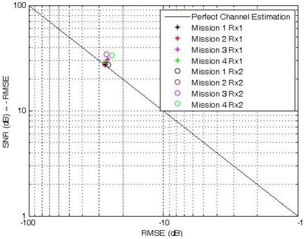
Figure 6.
SNR(dB) vs. RMSECE(dB) at the output of the channel estimator.
3.5. MIMO Deconvolution Results
A comparison of the MIMO deconvolution capability between experimental data and simulation results has been completed, using the metrics defined in Equations (29)–(31). The results are shown in Table 6 and Table 7. The impact of the parameter TL on the performance metrics is clearly observed. The results are shown for
 , which lead to the lowest RMSE values [17]. Both simulations and experimental results (averaged over the total number of missions carried out) are presented in Table 6. Clearly, RMSEMIMO_LE and RMSEMIMO_ICLE decrease as TL increases using either simulated or field data. Note that the equalizer length is limited to TL = 5.33 ms, as higher values of TL led to singularities.
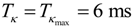
, which lead to the lowest RMSE values [17]. Both simulations and experimental results (averaged over the total number of missions carried out) are presented in Table 6. Clearly, RMSEMIMO_LE and RMSEMIMO_ICLE decrease as TL increases using either simulated or field data. Note that the equalizer length is limited to TL = 5.33 ms, as higher values of TL led to singularities.RMSEMIMO_LE, computed with both simulated and experimental data, is shown in Figure 7. Figure 7 shows the influence of the pre-cursor and post-cursor length: if TL is sufficiently large to provide accurate channel estimation, RMSEMIMO_LE drops as Tk increasing. Therefore, showing the influence of TL on RMSEMIMO_LE is not of great interest: this is why we chose to represent RMSEMIMO_LE as a function of Tk only (TL = 5.33 ms). For example, for an equalizer length TL = 5.33 ms, RMSEMIMO_LE = −6.2 dB with Tk = 0.7 ms and drops to RMSEMIMO_LE = −20.5 dB with Tk = 6.0 ms. As it has been shown in the channel estimation process results, the confidence interval also narrows as the process gets more and more reliable.
Table 6.
RMSE between emitted and (Raw) received signals, RMSEMIMO_Raw as a function of TL.
| TL (ms) | RMSE MIMO_Raw (dB) | |
|---|---|---|
| Simulations | Experiments | |
| 0.667 ms, 1.333 ms, 2 ms, 2.667 ms, 3.333 ms, 4 ms, 4.667 ms, 5.33 ms | 0.04 | 3 |
Table 7.
RMSE between emitted and received Signals after LE processing, RMSEMIMO_LE and after ICLE processing, RMSEMIMO_ICLE as functions of TL.
| RMSE MIMO_Raw (dB) | RMSE MIMO_ICLE (dB) | ||||
|---|---|---|---|---|---|
| Simulations | Experiments | Simulations | Experiments | ||
| TL (ms) | 0.667 | 0.4 | 19.7 | −4.5 | 15.8 |
| 1.333 | −3.4 | 14.4 | −6.7 | 12.1 | |
| 2.0 | −10.3 | 8.3 | −13 | 6.4 | |
| 2.667 | −20.5 | 5.5 | −33.4 | 3.1 | |
| 3.333 | −20.5 | 2.2 | −33.4 | 0.7 | |
| 4.0 | −20.5 | −1.9 | −33.3 | −3 | |
| 4.667 | −20.5 | −3.9 | −33.3 | −8.8 | |
| 5.33 | −20.5 | −3.3 | −33.2 | −26.9 | |
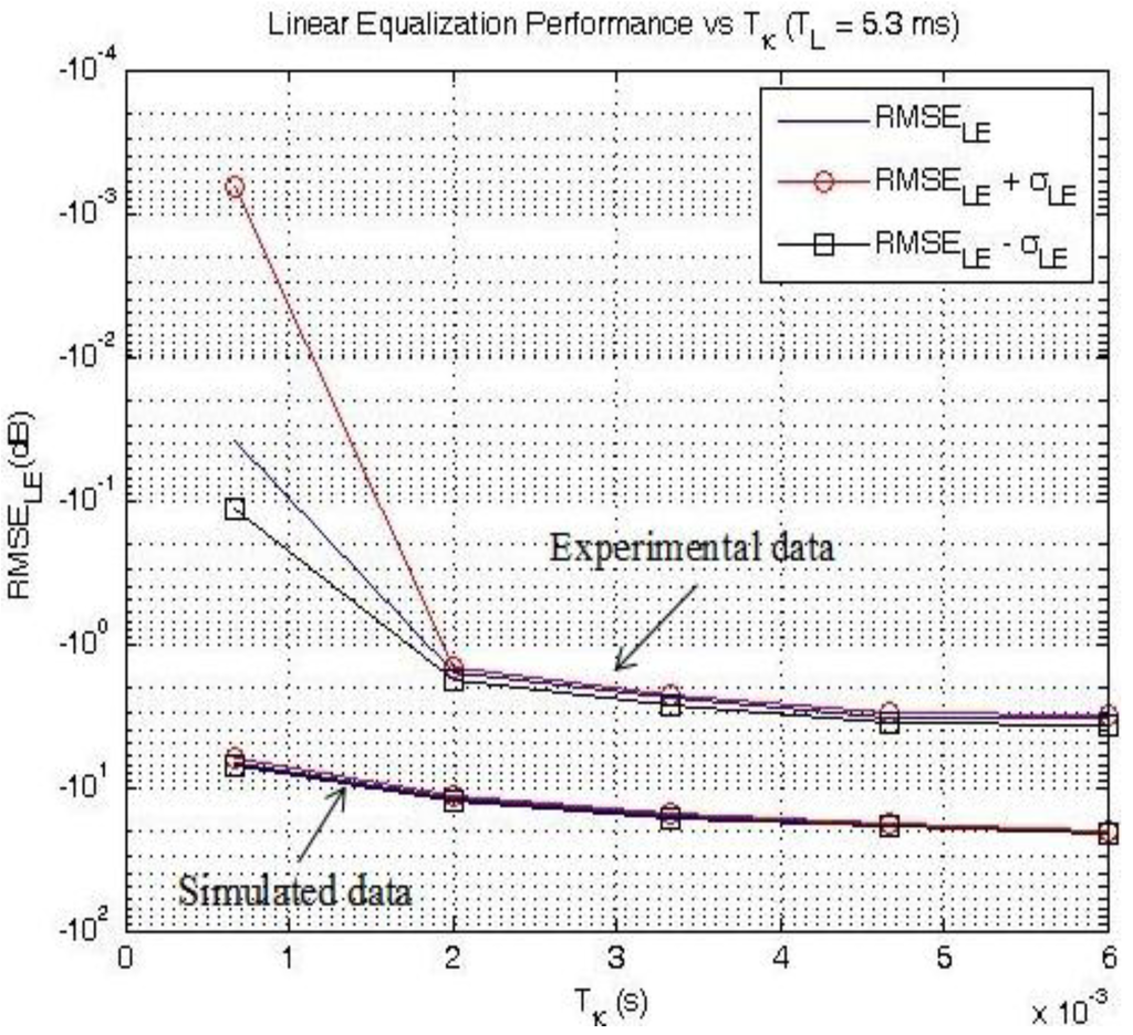
Figure 7.
RMSEMIMO_LE as a function of TL and Tk using simulated data.
In the case of experimental data, severe distortions in the received signals impact the accuracy of the MIMO deconvolution process. Indeed, Tk = 6.0 ms varies dramatically when computed with simulation and experimental data. In the best case scenario, we use TL = 5.33 ms and Tk = 6 ms. Table 7 shows that RMSEMIMO_LE = −3.9 dB using real data vs. RMSEMIMO_LE = −20.5 dB using simulated data. Nevertheless, the LE process on experimental data dramatically improves the quality of the received signal: Table 6 shows that RMSEMIMO_Raw = 3 dB whereas Table 7 shows that RMSEMIMO_LE = −3.3 dB when TL = 5.33 ms.
The relatively significant differences between simulation and field data performances are related to the time-varying characteristics of the experimental channel but also to co-antenna interferences. Indeed, the experimental channel impulse responses presented a coherence time much shorter than in the simulation case, leading to a lack of accuracy in the co-antenna interference removal process. Figure 8 shows the variation of RMSEMIMO_ICLE as a function of TL: if the MIMO sequence is known, the accuracy of the process improves as TL increases. On average, RMSEMIMO_ICLE = −26.9 dB when TL = 5.33 ms using experimental data vs. −33.2 dB using simulated data.
Figure 8.
RMSEMIMO_ICLE and RMSEMIMO_ICLE ± σICLE as a function of TL.
As expected, the comparisons between RMSEMIMO_ICLE and RMSEMIMO_LE calculated using simulated and experimental data reveals that LE process does not reach the lower bound provided by ICLE structure. Using simulation data, we find that RMSEMIMO_ICLE = −33.2 dB while RMSEMIMO_LE = −20.5 dB. This phenomenon is especially pronounced in the case of experimental data, where RMSEMIMO_ICLE = −26.9 dB and RMSEMIMO_LE = −3.3 dB for TL = 5.33 ms. One can conclude that LE alone is not totally sufficient to remove the whole interference terms provided by the frequency selective channel and multi-antenna architecture. Non-linear approaches like iterative processing strategy or decision feedback equalization appear thus necessary.
4. Conclusions
The capability of Hermes to support MIMO technology was presented in this paper. The system performance was evaluated using both simulated and experimental data, using two sources and two receivers. The ability to retrieve emitted messages, using a Linear Equalizer (LE), in the presence of inter-symbol interferences, co-antenna interferences and noise was estimated.
The channel impulse response estimation performance was related to the value of the channel estimate length TL. Computer simulations showed that for TL ≥ 2.667 ms, the relative root mean-square error used to measure the accuracy of the estimation reached a plateau. In this configuration, the RMSE (labeled RMSECE (dB)) between the received MIMO header and the MIMO header convolved with the estimated channel (averaged across every message and every receiver) was equal to −34.8 dB. This performance was compared to experimental data: in this case the same metric was equal to −25.7 dB for TL = 5.33 ms, indicating that the proposed technique evaluated fairly accurately the acoustic channel between every source and receiver.
To measure the benefits of this linear equalizer, the RMSE between emitted and received messages was first computed for each individual source and receiver. An Interference Cancelation Linear Equalizer (ICLE) was also developed to measure the limit of the deconvolution process, using estimated channel impulse responses. Optimized under the MMSE criterion, the ICLE took advantage of the known source signal. Using simulated data, TL = 5.33 ms and Tk = 6 ms, the RMSE was estimated at 0.03 dB before equalization (labeled RMSEMIMO_Raw (dB)), −20.5 dB after LE (labeled RMSEMIMO_LE (dB)) and −33.3 dB after ICLE (labeled RMSEMIMO_ICLE (dB)). For experimental data (with the same values for TL and Tk), the RMSE was estimated at −3 dB before equalization, −3.3 dB after LE and to −26.9 dB after ICLE.
To conclude with the results presented in this paper, the channel estimator and ICLE processes produce fairly similar results in simulation and experimentations. The fact that the performance of the channel estimation process and the ICLE are very comparable indicates that the deconvolution process is very accurate; in this case, the residual errors are not due to the ICLE itself. The LE performs better with simulated data but still brings some benefits to the communication system in the case of field data. The encouraging results indicate that the FAU Hermes underwater acoustic modem could be successfully equipped with MIMO technology.
Acknowledgments
This work is sponsored by the Office of Naval Research, Code 321 OE.
Conflicts of Interest
The authors declare no conflict of interest.
References
- Beaujean, P.P.J.; Carlson, E.A. HERMES a high bit-rate underwater acoustic modem operating at high frequencies for ports and shallow water applications. Mar. Technol. Soc. J. 2009, 43, 21–32. [Google Scholar] [CrossRef]
- Beaujean, P.P.; Carlson, E. Combined Vehicle Control, Status Check and High-Resolution Acoustic Images Retrieval Using a High-Frequency Acoustic Modem on a Hovering AUV. In Proceedings of OCEANS 2010, Seattle, WA, USA, 20–23 September 2010; pp. 1–10.
- Beaujean, P.P. A Performance Study of the High-Speed, High-Frequency Acoustic Uplink of the Hermes Underwater Acoustic Modem. In Proceedings of OCEANS 2009-EUROPE, Bremen, Germany, 11–14 May 2009; pp. 1–6.
- Real, G.; Beaujean, P.P.; Bouvet, P.J. A Channel Model and Estimation Technique for MIMO Underwater Acoustic Communications in Ports and Very Shallow Waters at very High Frequencies. In Proceeding of OCEANS 2011, Waikoloa, HI, USA, 19–22 September 2011; pp. 1–9.
- Tao, J.; Zheng, Y.R.; Xiao, C.; Yang, T.C.; Yang, W.B. Time-Domain Receiver Design for MIMO Underwater Acoustic Communications. In Proceedings of OCEANS 2008, Quebec City, QC, USA, 15–18 September 2008; pp. 1–6.
- Tuchler, M.; Singer, A.C.; Koetter, R. Minimum mean squared error equalization using a priori information. IEEE Trans. Signal Process. 2002, 50, 673–683. [Google Scholar] [CrossRef]
- Bouvet, P.J.; Hélard, M.; le Nir, V. Simple iterative receivers for MIMO LP-OFDM systems. In Annales des telecommunications; Springer-Verlag: Berlin, Germany, 2006; Volume 61, pp. 578–601. [Google Scholar]
- Bouvet, P.J.; Loussert, A. Capacity Analysis of Underwater Acoustic MIMO Communications. In Proceedings of OCEANS 2010 IEEE-Sydney, Sydney, Australia, 24–27 May 2010; pp. 1–8.
- Kilfoyle, D.B.; Preisig, J.C.; Baggeroer, A.B. Spatial modulation experiments in the underwater acoustic channel. IEEE J. Ocean. Eng. 2005, 30, 406–415. [Google Scholar] [CrossRef]
- Roy, S.; Duman, T.M.; McDonald, V.; Proakis, J.G. High-rate communication for underwater acoustic channels using multiple transmitters. IEEE J. Ocean. Eng. 2007, 32, 663–688. [Google Scholar] [CrossRef]
- Li, B.; Huang, J.; Zhou, S.; Ball, K.; Stojanovic, M.; Freitag, L.; Willett, P. MIMO-OFDM for high-rate underwater acoustic communications. IEEE J. Ocean. Eng. 2009, 34, 634–644. [Google Scholar] [CrossRef]
- Ceballos Carrascosa, P.; Stojanovic, M. Adaptive channel estimation and data detection for underwater acoustic MIMO-OFDM systems. IEEE J. Ocean. Eng. 2010, 35, 635–646. [Google Scholar] [CrossRef]
- Song, A.; Badiey, M. Time reversal multiple-input/multiple-output acoustic communication enhanced by parallel interference cancellation. J. Acoust. Soc. Am. 2012, 131, 281–291. [Google Scholar] [CrossRef]
- Stojanovic, M.; Catipovic, J.A.; Proakis, J.G. Phase-coherent digital communications for underwater acoustic channels. IEEE J. Ocean. Eng. 1994, 19, 100–111. [Google Scholar] [CrossRef]
- Li, J.; Stoica, P.; Zheng, X. Signal synthesis and receiver design for MIMO radar imaging. IEEE Trans. Signal Process. 2008, 56, 3959–3968. [Google Scholar] [CrossRef]
- Song, A.; Badiey, M.; McDonald, V.K. Multi-Channel Combining and Equalization for UWA MIMO Channels. In Proceedings of IEEE Oceans Conference, Quebec City, QC, USA, 15–18 September 2008; pp. 1–6.
- Real, G. Very High Frequency, MIMO Underwater Acoustic Communications in Ports and Shallow Waters. Master’s Thesis, Florida Atlantic University, FL, USA, 2011. [Google Scholar]
- Proakis, J.G. Digital Communications, 4th ed.; McGraw-Hill: New York, NY, USA, 2000. [Google Scholar]
- Laot, C.; le Bidan, R.; Leroux, D. Low-complexity MMSE turbo equalization: a possible solution for EDGE. IEEE Trans. Wirel. Commun. 2005, 4, 965–974. [Google Scholar] [CrossRef]
- Medwin, H.; Clay, C.S. Fundamentals of Acoustical Oceanography; Academic Press: Waltham, MA, USA, 1997. [Google Scholar]
© 2013 by the authors; licensee MDPI, Basel, Switzerland. This article is an open access article distributed under the terms and conditions of the Creative Commons Attribution license (http://creativecommons.org/licenses/by/3.0/).