Digital Trade Feature Map: A New Method for Visualization and Analysis of Spatial Patterns in Bilateral Trade

Abstract

Product bilateral trade features can be organized and expressed in the Cartesian coordinate system by taking imports and exports as X and Y, which is similar to spatial visualization. Hence, geospatial expression and analysis methodologies can be applied in bilateral trade studies. In this paper, we propose a new digital trade feature map (DTFM) method for the visualization of bilateral trade features from a spatial perspective. The implementation process of DTFM can be summarized as feature extraction, visualization, and analysis. China–US bilateral trade data were used in several case studies. As the case studies show, the DTFM has the advantages of clear expression, easy operationalization and is highly extensible. Moreover, this method can provide a broader perspective for the understanding of trade features, i.e., in comprehensively considering the features of a specific product type and its neighbors. Furthermore, we propose an extensible DTFM application framework into which different trade features, different grid generation modes, and numerous spatial analysis models can be readily integrated.

1. Introduction

In the present era of globalization, trade is considered an important catalyst for the growth and development of many nations. Despite the adverse effects of trade barriers and export controls, the development of inter-product and intra-product trade research plays an important role in enhancing the understanding of the trade relationship structure, evolution, and relevant driving factors.

The analysis and visualization of the trade features of numerous different product types at small scales is a challenge for many studies. On the one hand, numerous indexes were proposed from the neo-classical trade theory and the new international trade theory, and widely used in the analysis of international trade relationships and attributions. For instance, [1] used the revealed comparative advantage index (RCAI) [2] to analyze comparative advantage products and their interactions with production structure and product diversification between the European Union (EU-27) and the European Neighborhood Policy countries. [3] used an export dependency index to measure the relative exposure of sectors and countries in Latin America to fluctuations of Chinese demand. The concentration index and Grubel–Lloyd index have been used to analyze the influence of free trade agreements on the diversification of exports from Latin America [4] and the dynamics of intra-industry trade flows in MENA (Middle Eastern and Northern Africa) countries [5], respectively. The technical complexity index, trade complementarity index, and export similarity index have been comprehensively applied in the comparison of industrial competitive advantages/disadvantages and the analysis of trade structure and its changing trends, as well as to evaluate the national position in the international industrial value chain among multiple economies. However, most of these index-based approaches are appropriate only for a comparison of products or industries of the same type among multiple countries. It is difficult to express the trade features of numerous different product types in small scales. Furthermore, intra-product trade information will be smoothened if we classify thousands of traded products into several industries or broad categories.

On the other hand, complex network analysis methods and complexity theory provide research paradigm for revealing insights into the structure and evolution of trade relationships and interdependencies between trade partners that are not immediately evident in a purely statistical analysis of trade data. For most studies [6,7,8,9], networks were constructed by taking countries (or regions) as nodes, trade flows as edges, and trade features (trade volume, RCAI) as weights to express trade relationships, and their driving factors of specific categories of products (e.g., wind renewable energy industry [10,11], iron ore products [12], agricultural products [9,13]) among different countries. For instance, Cristelli [6] quantified export similarity by building distance matrices for products and countries based on the complex network theory and then determining the evolution of competitors’ communities. Ermann [7] indicated that trade networks are characterized by being high-nested, which is typical of ecological networks. Given this, he constructed a Google matrix G of the multiproduct world trade between the United Nations (UN) countries to analyze the properties of trade flows [8]. Dong [9] constructed wheat-trading competition networks to analyze the impact of climate change on the global trade flows of wheat by ultimately putting forward a policy framework to promote a stable and healthy wheat-trading environment. The number of products is still a constraint that cannot be ignored for these studies, even though it can be somewhat increased by constructing multilayer networks [14,15]. Some studies developed two-mode network models to express the relationships among numerous categories of products [16,17,18,19]. Hildago [17] presents the concept of “product space”, in which products that can be produced in tandem (i.e., products that ‘require similar institutions, infrastructure, physical factors, technology, or some combination thereof’) are closely distributed with each other in the two-mode network. Given that, links of countries and products were integrated into a “product space” network to evaluate the complexity of national productive structures [18,20]. Hausmann takes economic complexity as a measure of society’s productive knowledge and thereby expresses each country’s adjacent possible or potential new products through the graphical representation of the “product space” [21]. These studies [17,18,20,21] are creative and of great significance for trade features analysis and visualization. However, the network of these hundreds of products is too complicated to identify specific products for visualization, and it is hard to clearly express the differences in trade features among different countries or phases. The same disadvantage also exists in two other widely used product trade pattern analysis models, i.e., the gravity model [22,23,24] and the clustering model [25].

The above methods significantly influence the understanding and analysis of the trade relationship structures or trade flow characteristics of products (or industries) across multiple countries. However, trade differentiation characteristics and the change processes of thousands of products are difficult to express clearly. Hence, it is of significance to develop methods that can analyze and express bilateral trade patterns and the evolution of many types of products [20]. Over recent years, geographic information science has been used to provide significant theories and methods for the analysis of the spatial differentiation characteristics and spatiotemporal variations of land surface elements [26,27,28]. The spatial coordinate is important factor for spatial analysis and visualization. Although the bilateral trade data of products has a unique classification system and quantitative expression mode, the trade volume of product can be organized and expressed in Cartesian coordinate system by taking imports and exports as X and Y, which is similar to spatial visualization of land surface elements. On this basis, spatiotemporal analysis models can be applied to product trade studies.

This study develops a common method with characteristics of high comparability, clear expression, easy operationalization for visualization and analysis of spatial patterns of many types of products. We propose a new digital trade feature map (DTFM) method for the visualization of bilateral trade features from a spatial perspective. China–US bilateral trade data are used in case studies. According to the DTFM method, ‘trade space’ is constructed using product imports and exports as the coordinate axis (unit: dollar). Each type of product is spatially transformed to a points set and expressed in the ‘trade space’ according to annual imports and exports. Then, trade features, including importance level and import–export difference class, are evaluated by spatial statistics and the head/tail breaks method. Lastly, a grid map is generated by the reverse application of the Hilbert curve generation method for the visualization of trade features. As the case studies show, the DTFM method possesses the advantages of clear expression, easy operationalization and is highly extensible. Therefore, we also propose an extensible DTFM application framework in which different trade features, different grid generation modes, and numerous spatial analysis models can be readily integrated.

2. Materials and Methods

2.1. Data

The UN International Trade Statistics Database (UN Comtrade) is the world’s largest and most widely used international trade database with a high degree of authority and uniformity. Its record date can point back to 1962, and its total recorded quantity exceeds 3 billion. Over 200 countries/areas (reporters) provide their annual international trade statistics data detailed by commodities/service categories and partner countries. The data are subsequently transformed into the UN Statistics Division standard format with consistent coding (e.g., HS (Harmonized Product Description and Coding System), SITC (Standard International Trade Classification) and BEC (Classification by Broad Economic Categories)) and valuation in the data loading process. In this paper, a China–US annual bilateral trade dataset was extracted from the database and applied to the development of methods and case studies for the DTFM. The dataset is reported by the Chinese maritime customs and covers 27 years of imports and exports (unit: U.S. dollar) from 1992 to 2018. Product types are classified and encoded in terms of the harmonized product description and coding system (HS) 4-digit coding rule. The HS 4-digit code is generated from further subdivision of the HS 2-digit code (see Table A1 for detailed HS 2-digit coding rule); the total number of product classes is 1256. It is important to note that there is ambiguity in the import and export trade; therefore, to avoid confusion, we stipulate that imports and exports presented in this paper represent China as reporter and USA as partner, respectively.

2.2. Trade Data Spatialization Method

Geospatial expression and analysis methodologies are also appropriate for bilateral trade studies. In this paper, trade space was proposed by using product imports and exports as the coordinate axis (unit: dollar). Then, different types of products were spatially transformed to a points set and expressed in the ‘trade space’ according to their annual imports and exports. For each type of product, the location of a point reflects its trade volume and difference between imports and exports in a certain year, whereas the degree of dispersion of the distribution of points reflects its degree of trade volume change during a certain period of time. China–US annual bilateral trade data from 1992 to 2018 were transformed and expressed as sample points in the ‘trade space’, as shown in Figure 1. Taking product M (gas compressor and fan, HS 4-digit code: 8414) as an example, the trade volume change degree of M (SD_M) can be quantified using Equation (1), wherein $x_{M,i}$ and $y_{M,i}$ present imports and exports, respectively, of M in the ith-year; $\overline{x_M}$ and $\overline{y_M}$ are the mean imports and exports during n years and n is the total number of years. The average trade intensity L_M of M during n years can be calculated using Equation (2), wherein l_M,i represents the annual trade intensity of M in the ith-year. In this way, the changing characteristics of product trade volume and their correlations with each other can be intuitively expressed as spatial migration or spatial aggregation. The value of both exports and imports of different products and the difference between them can be integrated displayed.

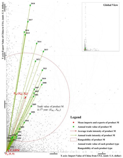
Figure 1. Variation in China–US bilateral trade in ‘trade space’. product M represents ‘Gas compressor and fan’, and its HS 4-digit code is 8414. By creating a line L that connects original point PO (0, 0) and central point P_M ($\overline{x_M}$, $\overline{y_M}$ ), the length of L indicates the average trade intensity of product M. The Angle C_LDM between the L- and X-axis indicates the import–export difference.

Next, we constructed the rank–size distribution [29] of SD_M and L_M, as shown in Figure 2a,c. The rank–size distributions of SD_M and L_M both express significant characteristics of a heavy tail [30], i.e., products with large values are of low frequency and constitute the ‘head’, whereas products with small values are of high frequency and constitute the ‘tail’. As Figure 2b,d shows, the probability density function (PDF) has a linear distribution when graphed as a double-logarithm plot, i.e., the distributions of SD_M and L_M can be represented by the power law. A heavy-tailed distribution can also be observed when assessing the PDFs of SD_M and L_M. It should be noted that low-frequency events are present in the head in rank–size distributions but are present in the tail in PDFs. In this article, to avoid confusion, the terms head and tail refer to those of the rank–size distribution rather than those of the PDF.

$$S{D}_M=\sqrt{\frac{{\sum }_{i=1}^n{\left(x_{M,i}-\overline{x_M}\right)}^2}{n}+\frac{{\sum }_{i=1}^n{\left(y_{M,i}-\overline{y_M}\right)}^2}{n}}$$

(1)

$$L_M=\frac{{\sum }_{i=1}^n{l}_{M,i}}{n},l_{M,i}=\sqrt{x_{M,i}{}^2+y_{M,i}{}^2}$$

(2)

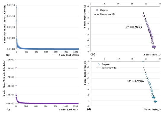
Figure 2. Heavy-tailed distributions of SD_M and L_M. (a) Rank–size distribution of SD_M. (b) Probability density distribution (Log) of SD_M. (c) Rank–size distribution of L_M. (d) Probability density distribution (Log) of L_M.

2.3. Head/Tail Breaks Method

In this study, the heavy-tailed distribution of products’ bilateral trade features was considered in the level-classification process. Unlike a normal distribution that has two thin tails that rapidly reach the x-axis, a heavy-tailed distribution, theoretically, has a long tail skewed to the right, approaching but never touching the x-axis. Heavy-tailed distributions have been widely observed for social and natural phenomena [30]. For instance, 10% of the land in Europe is urban, and 90% is countryside; whereas, 80% of people in Europe are urban residents, and 90% of land is owned by 20% of the population, i.e., the smaller area with a large population constitutes the ‘head’, whereas the ‘tail’ is composed of the larger area with a small population. Similar phenomena are social wealth distribution and architectural environments [31,32]. Traditional classification methods are dominated by a Gaussian approach [33,34,35]; they focus on high-frequency events and consider low-frequency events to be separated from high-frequency events [36]. There exist large gaps or breaks between high-frequency and low-frequency values, as well as between different levels of low-frequency values, which constitute the foundation for the natural break classification [37]. However, for a heavy-tailed distribution, low-frequency events contain far more information and tend to be more important than high-frequency events [37]. For instance, there are numerous rare and extreme events in nature, society, and our daily lives that are termed ‘black swan events’ [38].

For the imbalance of a heavy-tailed distribution, Jiang formulated the head/tail division rule: ‘Given a variable X, if its values follow heavy-tailed distribution, then the mean of the values can divide all the values into two parts: a high percentage in the tail, and a low percentage in the head’ [30]. Under this rule, Jiang proposed the head/tail breaks method for data classification and verified its advantages over the natural break method [39]. The head/tail breaks method partitions the data values into two groups around the arithmetic mean and continues to iteratively partition the values above the mean until the ‘head’ values are no longer heavy-tailed distributed. Therefore, the number of classes and the class intervals are both naturally determined by the fractal nature of the heavy-tailed distribution of the data. The rank–size distribution of SD_M was used as sample data and was classified into five levels according to the head/tail breaks method, as shown in Figure 3, in which a higher level indicates a more important product.

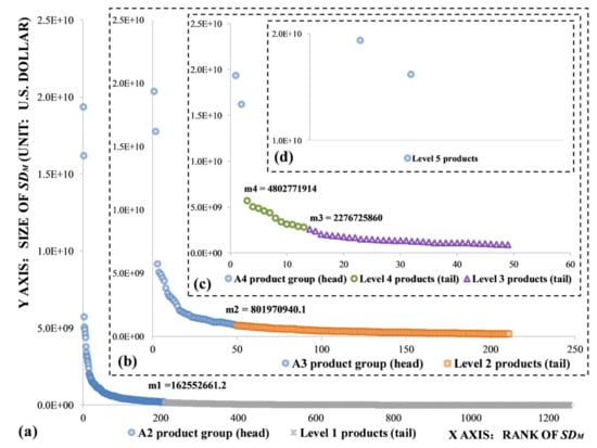
Figure 3. Classification process of the rank–size distribution of SD_M based on the head/tail breaks. (a) Extract Level 1 products–m1 is the arithmetic mean of all SD_M values; values above m1 were extracted as an A2 product group (head), and the rest as Level 1 products (tail). (b) Extract Level 2 products–m2 is the arithmetic mean of A2 values0; values above m2 were extracted as an A3 product group (head), and the rest as Level 2 products (tail). (c) Extract Level 3, 4 products in sequence. (d) Define Level 5 products.

2.4. Hilbert Curve-Based Products Grids Generation Method

A Hilbert curve is a continuous curve that has self-similar properties and a zigzag and non-differentiable structure. This type of curve can uninterruptedly traverse each cell of a $2^n*2^n$ square grid system. Any two cells traversed sequentially are also adjacent in space. Hence, the Hilbert curve can be used to map elements in a two-dimensional space to a one-dimensional linear space while preserving the proximity among the elements as much as possible. Because of the spatial correlation characteristics of geographical elements, the Hilbert curve has been widely used in geographic data processing and management, e.g., in raster data compression [40,41,42], spatial indexing [43], and data segmentation [44]. In this paper, a products grid generation method was proposed by the reverse dimension increasing application of the Hilbert curve. A scanning matrix generation method (SMG) [45] was applied for the construction of a Hilbert curve. According to the SMG, an n-order ($2^n\times 2^n$) scanning matrix $H_{2^n}$ can be generated quickly and accurately by a degree elevation iterative algorithm based on a 1-order ($2^1\times 2^1$) matrix $H_2$, as shown in Equation (3). The Hilbert curve can then be generated by connecting the matrix element values in ascending order, as shown in Figure A1.

$${\mathrm{H}}_{2^{\mathrm{k}+1}}=\left\{\begin{array}{cc}\left[\begin{array}{cc}{\mathrm{H}}_{2^{\mathrm{k}}}& 4^{\mathrm{k}}{\mathrm{E}}_{2^{\mathrm{k}}}+{\mathrm{H}}_{2^{\mathrm{k}}}^{\mathrm{T}}\\ \left(4^{\mathrm{k}}+1\right){\mathrm{E}}_{2^{\mathrm{k}}}-\overline{{\mathrm{H}}_{2^{\mathrm{k}}}}& \left(3\times 4^{\mathrm{k}}+1\right){\mathrm{E}}_{2^{\mathrm{k}}}-{\left(\tilde{{\mathrm{H}}_{2^{\mathrm{k}}}}\right)}^{\mathrm{T}}\end{array}\right]& \begin{array}{c}\mathrm{k} \mathrm{is} \mathrm{an} \mathrm{even} \mathrm{number}\end{array}\\ \left[\begin{array}{cc}{\mathrm{H}}_{2^{\mathrm{k}}}& \left(4^{\mathrm{k}+1}+1\right){\mathrm{E}}_{2^{\mathrm{k}}}-\tilde{{\mathrm{H}}_{2^{\mathrm{k}}}}\\ 4^{\mathrm{k}}{\mathrm{E}}_{2^{\mathrm{k}}}+{\mathrm{H}}_{2^{\mathrm{k}}}^{\mathrm{T}}& \left(3\times 4^{\mathrm{k}}+1\right){\mathrm{E}}_{2^{\mathrm{k}}}-\left({\mathrm{H}}_{2^{\mathrm{k}}}^{\mathrm{T}}\right)\end{array}\right]& \begin{array}{c}\mathrm{k} \mathrm{is} \mathrm{an} \mathrm{odd} \mathrm{number}\end{array}\end{array}\right.$$

$$\mathrm{thereunto}, H_2=\left[\begin{array}{ll}2& 3\\ 1& 4\end{array}\right], \mathrm{set} H_m=\left[\begin{array}{lll}\begin{array}{ll}{a}_{1 ,1}& a_{1 ,2}\\ a_{2 ,1}& a_{2 ,1}\end{array}& \cdots & \begin{array}{l}{a}_{1 ,m}\\ a_{2,m}\end{array}\\ ⋮& \ddots & ⋮\\ \begin{array}{ll}{a}_{m ,1}& a_{m ,1}\end{array}& \cdots & a_{m ,m}\end{array}\right]$$

$$\widetilde{{\mathrm{H}}_{\mathrm{m}}}=\left[\begin{array}{lll}\begin{array}{ll}{\mathrm{a}}_{1 ,\mathrm{m}}& {\mathrm{a}}_{1 ,\mathrm{m}-1}\\ {\mathrm{a}}_{2 ,\mathrm{m}}& {\mathrm{a}}_{2 ,\mathrm{m}-1}\end{array}& \cdots & \begin{array}{l}{\mathrm{a}}_{1 ,1}\\ {\mathrm{a}}_{2 ,1}\end{array}\\ ⋮& \ddots & ⋮\\ \begin{array}{ll}{\mathrm{a}}_{\mathrm{m} ,\mathrm{m}}& {\mathrm{a}}_{\mathrm{m} ,\mathrm{m}-1}\end{array}& \cdots & {\mathrm{a}}_{\mathrm{m} ,1}\end{array}\right], \overline{{\mathrm{H}}_{\mathrm{m}}}=\left[\begin{array}{lll}\begin{array}{ll}{\mathrm{a}}_{\mathrm{m} ,1}& {\mathrm{a}}_{\mathrm{m} ,2}\\ {\mathrm{a}}_{\mathrm{m}-1 ,1}& {\mathrm{a}}_{\mathrm{m}-1 ,2}\end{array}& \cdots & \begin{array}{l}{\mathrm{a}}_{\mathrm{m} ,\mathrm{m}}\\ {\mathrm{a}}_{\mathrm{m}-1 ,\mathrm{m}}\end{array}\\ ⋮& \ddots & ⋮\\ \begin{array}{ll}{\mathrm{a}}_{1 ,1}& {\mathrm{a}}_{1 ,2}\end{array}& \cdots & {\mathrm{a}}_{1 ,\mathrm{m}}\end{array}\right]$$

(3)

For 1256 types of China–US bilateral trade products, it is hard to comprehensively express the differences in product types, SD_M and L_M, in a one-dimensional space. By the reverse application of SMG, the HS 4-digit codes of products can be mapped to a two-dimensional space and visualized in a grid system. The implementation process is listed as follows.

Step 1: by applying SMG, a 6-order ($2^6\times 2^6$) scanning matrix ${\mathit{H}}_{{\mathbf{2}}^{\mathbf{6}}}$ and its corresponding Hilbert curve were generated. Each matrix element can be considered as a node of the Hilbert curve with a unique serial number that is sorted in ascending order starting at one. It means that the initial node and terminal node of the Hilbert curve, respectively, has the minimum (1) and maximum (4096) serial number.

Step 2: construct a vector format-based (*.shp) $2^6\times 2^6$ grid system ${\mathit{V}}_{{\mathbf{2}}^{\mathbf{6}}}$, and create a new field named ‘comtrade’ for this file.

Step 3: assign the serial number of each matrix element in ${\mathit{H}}_{{\mathbf{2}}^{\mathbf{6}}}$ to the field ‘comtrade’ attribute of the corresponding grid with the same row and column number in ${\mathit{V}}_{{\mathbf{2}}^{\mathbf{6}}}$ by developing an ArcObjects-based application (see ${\mathit{V}}_{{\mathbf{2}}^{\mathbf{6}}}$ in Supplementary Materials).

Step 4: the 1256 types of products were also sorted in ascending order according to their HS 4-digit codes.

Step 5: the first 1256 grids of ${\mathit{V}}_{{\mathbf{2}}^{\mathbf{6}}}$ were extracted.

Step 6: for each grid, its field ‘comtrade’ attribute w (w = 1, 2…1256) was replaced with the HS 4-digit code of the w product in the order. In this way, the HS 4-digit codes of products can be mapped to a two-dimensional space and visualized on a grid system.

As Figure 4 shows, similar types of products are distributed in neighboring grids according to their HS 4-digit codes. Hence, our method provides a broader perspective for understanding and analyzing trade features. We accomplish this by comprehensively considering the features of a specific type of product and its neighbors, which is difficult to achieve using other methods, such as index-based approaches or complex network analysis methods.

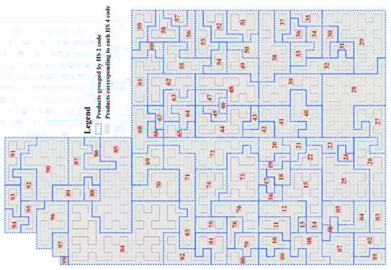
Figure 4. HS 4-digit code grid system. Each type of HS 4-digit code product corresponds to one grid, and the marked number is the HS 2-digit code of the product category to which it belongs. See Figure A2 for details of the HS 6-digit code grid system.

We considered that the reverse dimension increasing application of the Hilbert curve has better adaptability than dimension reduction applications. Firstly, the two-dimensional matrix must be organized in the form of $2^n*2^n$ for dimensionality reduction applications, whereas dimension increasing can be applied on any one-dimensional array. Secondly, neighboring elements in two-dimensional space may become distant from each other through dimension reduction, whereas neighboring relationships can be maintained by dimension increasing. Furthermore, the reverse dimension increasing application of the Hilbert curve has an advantage of high versatility and will not be restricted by the number of product categories or variation of trade features.

3. Case Studies

3.1. Case Study 1: Spatial Pattern Analysis of Product Importance Level

The spatial pattern of the product importance level in the China–US bilateral trade was calculated using the DTFM method, as shown in Figure 5. The head/tail breaks method was used to classify the rank–size distribution of SD_M and L_M into five levels (Figure 2). High-level product types contain far more information and tend to be more important than low-level product types. The comparison shows that the classification results for SD_M (Figure 3) are nearly in accordance with those of L_M. Hence, for each product type, its importance level was set as the maximum SD_M level and L_M level to maintain the presence of high-level product types as much as possible.

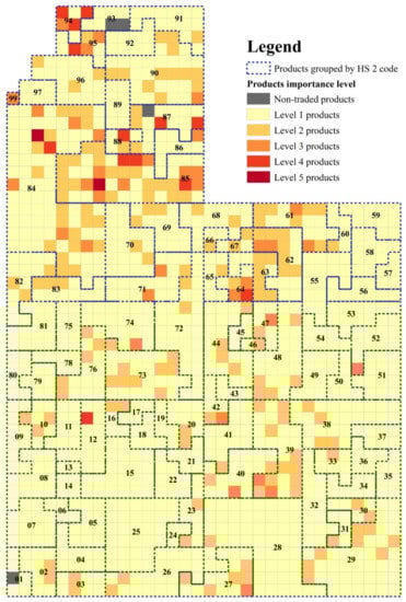
Figure 5. Spatial pattern of product importance level in China–US bilateral trade.

According to Figure 5, nearly 83% of Level 1 product types constitute the ‘tail’, supporting the overall stability of the China–US bilateral trade. The ‘head’ (Levels 2–5) consists of less than 17% of the product types; these types are important in China–US trade relations. Level 5 products are ‘automatic data processing machines (computers)’ (HS 4-digit code: 8471) and ‘electric apparatus for line telephony, telegraphy’ (HS 4-digit code: 8517). Level 3 and 4 products are mainly intensively located in product categories whose HS 2-digit codes are 61–64 (‘textile products’), 87 (‘vehicles, other than railway or tramway rolling stock’), 88 (‘aircraft, spacecraft and parts thereof’), 90 (‘optical, photographic, cinematographic, measuring, checking, medical or surgical instruments and apparatus’) and 94 and 95 (‘furniture, toys, games and sports requisites’). Meanwhile, a few Level 3 and 4 product types show discrete distributions; their corresponding HS 4-digit codes are 1201 (soya beans), 4011 (new pneumatic tires, of rubber), 4707 (waste or scrap of paper or paperboard), 5201 (cotton, not carded or combed), 7108 (gold, unwrought, semi-manufactured, powder form), 7113 (jewelry and parts, containing precious metal), and 7404 (copper, copper alloy, waste, or scrap).

In conclusion, the DTFM provides a uniform and normative grid system for expressing trade features. Bilateral trade features of plentiful different types of products are clearly expressed. The relatively more important product types of the China–US bilateral trade mainly fall into technology-intensive product categories (such as machinery, electrical appliances, aerospace, communications, optics and medicine) and some labor-intensive product categories (such as furniture, toys, and textiles). Product levels in the former type are highly diversified because of significant component assembly and processing in intra-product trade. While for the latter, the highly diverse patterns in products levels are caused by high market demand.

3.2. Case Study 2: Spatial Pattern Analysis of Product Import–Export Difference Class

For each type of product M, its import–export difference C_LDM during n years can be calculated by Equation (4), wherein $x_{M,i}$ and $y_{M,i}$ represent imports and exports, respectively, of M in the ith-year; n is the total number of years. C_LDM is directly proportional to the ratio of total exports to total imports. If total exports of M are equal to its total imports, C_LDM is 45 (unit: degrees). If C_LDM∈[0, 45), total exports of M are less than its total imports. In this instance, the rank–size distribution of cot(C_LDM) shows significant characteristics of a heavy tail. Similarly, the rank–size distribution of tan(C_LDM) can be observed as a heavy-tailed distribution when C_LDM∈(45, 90], as shown in Figure A3. Hence, the ratio of total exports to total imports varies markedly for different intervals of C_LDM. The head/tail breaks method was used with manual amendment to place the rank–size distributions of cot(C_LDM) and tan(C_LDM) into five classes, as shown in Table 1. Ultimately, we constructed a color mapping space to synthetically express product importance level and import–export difference class on a grid system, as shown in Figure 6.

Table 1. Head/Tail Breaks intervals of C_LDM.

No.	Class	C_LDM Intervals	Illustration
1	Class A	[85, 90]	Sexp1 >> Simp2, Sexp / Simp > 11.43
2	Class B	(60, 85)	Sexp > Simp, Sexp / Simp ∈ (1.73,11.43]
3	Class C	[30, 60]	Sexp ≈ Simp, Sexp / Simp or Simp / Sexp ∈ [1,1.73]
4	Class D	(5, 30)	Sexp < Simp, Simp / Sexp ∈ (1.73,11.43]
5	Class E	[0, 5]	Sexp << Simp, Simp / Sexp > 11.43

¹ total exports, ² total imports

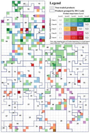
Figure 6. Spatial pattern of product import–export difference class. Only the import–export difference class information about high-level products (importance level > 1) were expressed in this figure. See Figure A4 for detailed information.

For important (Level > 1) products, those with surplus characteristics (Class A/B) are more likely to appear as a local aggregation distribution. These products are intensively located in product categories whose HS 2-digit codes are 61–64, 73, 76, 84, 85, 94, and 95. In ‘machinery and mechanical appliances’ (84) and ‘electrical machinery and equipment’ (85), the distributions of high-level Class A/B products (H-SPs) and high-level Class D/E products (H-DPs) are mixed. H-SPs are manufactured goods at the end of the value chain (low profit), whereas H-DPs are mostly components in the upper region of the value chain. This mixed-status indicates that the trade penalty for these types of products may damage the interests of multiple participating countries in addition to China and the USA. However, H-SPs in ‘furniture, toys, textile products, steel products, aluminum products’ are distributed intensively at the end of the value chain with few neighboring H-DPs and low market access barriers. In the context of a contraction in market demand or where product supply can be taken over by other countries, trade penalties for these H-SPs will occur readily and intensively compromise China’s interests. On the contrary, H-DPs are more likely to appear with a discrete distribution. Most of these H-DPs are raw materials and components in the upstream industrial chain (e.g., ‘soya beans’ (1201), ‘waste or scrap of paper or paperboard’ (4707), ‘cotton, unwrought gold’ (5201) and ‘copper, copper alloy, waste, or scrap’ (7404)). A few H-DPs are manufactured goods, such as ‘motor vehicles for transport of persons (except buses)’ (8703) and ‘aircraft, spacecraft, satellites’ (8802). Raw materials and manufactured goods in these H-DPs have the characteristics of being easy to replace and having a small range of influence.

The import–export difference class information of some high-level products (Level > 2) is listed in Table 2. First, the distribution of these products is unbalanced; the quantity of H-SPs is significantly greater than that of H-DPs, which is directly shown as the trade surplus between China and the USA. Second, in the context of economic globalization, the China–US bilateral trade is closely intertwined and mutually influenced, with a clear division of complementary types. H-SPs are mainly manufactured goods with a strong dependence on market demand, whereas H-DPs are mainly raw materials and components with resource barriers or technical barriers. This phenomenon indicates that the USA can be regarded as China’s product sales market and origin of raw materials; therefore, taken as a whole, China does not have a market advantage in China–US trade conflicts. Furthermore, there are only two types of high-level Class C products. This indicates that product trade competitiveness is weak between these two countries. Furthermore, we visualized the different aggregation characteristics of products and their relationship with trade features from a broader perspective.

$$C\_LDM=\arctan \left(\frac{{\sum }_{i=1}^n{y}_{M,i}}{{\sum }_{i=1}^n{x}_{M,i}}\right)$$

(4)

Table 2. Import–export difference class information of some high-level products (Level > 2).

HS 4 Code	Type of Product	Class, Level	HS 4 Code	Type of Product	Class, Level
Surplus (Class A / B)			Deficit (Class D / E)
3924	Plastic table, kitchen, household, toilet articles	Class A, Level 3	1201	Soya beans	Class E, Level 4
3926	Plastic articles nes	Class A, Level 3	4707	Waste or scrap of paper or paperboard	Class E, Level 3
4011	New pneumatic tires, of rubber	Class A, Level 3	5201	Cotton, not carded or combed	Class E, Level 3
4202	Trunks, suitcases, camera cases, handbags, etc	Class A, Level 3	7108	Gold, unwrought, semi-manufactured, powder form	Class E, Level 3
6104	Women’s, girl’s suit, dress, skirt, etc, knit or crochet	Class A, Level 3	7404	Copper, copper alloy, waste or scrap	Class E, Level 3
6110	Jerseys, pullovers, cardigans, etc, knit or crochet	Class A, Level 3	8411	Turbo-jets, turbo-propellers/other gas turbine engine	Class D, Level 3
6203	Men’s or boy’s suits, jackets, trousers etc not knit	Class A, Level 3	8486	Machines and apparatus of a kind used solely or principally for the manufacture of semiconductor boules or wafers, semiconductor devices, electronic integrated circuits or flat panel displays; machines and apparatus specified in Note 9 (C) of this Chapter	Class E, Level 3
6204	Women’s, girl’s suits, jacket, dress, skirt, etc, woven	Class A, Level 3
6402	Footwear nes, with outer sole, upper rubber or plastic	Class A, Level 3
6403	Footwear with uppers of leather	Class A, Level 4	8542	Electronic integrated circuits and microassemblies	Class D, Level 4
6404	Footwear with uppers of textile materials	Class A, Level 3	8703	Motor vehicles for transport of persons (except buses	Class E, Level 4
7113	Jewelry and parts, containing precious metal	Class A, Level 3	8802	Aircraft, spacecraft, satellites	Class E, Level 4
8414	Air, vacuum pumps, compressors, ventilating fans, etc	Class B, Level 3	9018	Instruments etc for medical, surgical, dental, etc us	Class D, Level 3
8443	Printing and ancillary machinery	Class A, Level 3	Approximate (Class C)
8467	Tools for working in the hand, non-electric motor	Class A, Level 3	8541	Diodes, transistors, semi- conductors, etc	Class C, Level 3
8471	Automatic data processing machines (computers)	Class A, Level 5	2709	Petroleum oils, oils from bituminous minerals, crude	Class C, Level 3
8473	Parts, accessories, except covers, for office machine	Class B, Level 4	Surplus (Class A / B)
8481	Taps, cocks, valves for pipes, tanks, boilers, etc	Class B, Level 3	8544	Insulated wire and cable, optical fiber cable	Class B, Level 3
8504	Electric transformers, static converters and rectifier	Class B, Level 3	8609	Cargo containers designed for carriage of goods	Class A, Level 3
8516	Electric equipment with heating element, domestic etc	Class A, Level 3	8708	Parts and accessories for motor vehicles	Class B, Level 4
8517	Electric apparatus for line telephony, telegraphy	Class A, Level 5	9401	Seats (except dentist, barber, etc chairs)	Class A, Level 4
8518	Audio-electronic equipment, except recording devices	Class A, Level 3	9405	Lamps and lighting fittings, illuminated signs, etc	Class A, Level 4
8521	Video recording and reproducing apparatus	Class A, Level 3	9404	Mattress supports, mattresses, bedding	Class A, Level 3
8525	Radio and TV transmitters, television cameras	Class A, Level 4	9403	Other furniture and parts thereof	Class A, Level 4
8528	Television receivers, video monitors, projectors	Class A, Level 4	9503	Other toys, scale models, puzzles, etc	Class A, Level 4
8529	Parts for radio, TV transmission, receive equipment	Class B, Level 3	9504	Articles for funfairs, table and parlor games	Class A, Level 3
8543	Electrical machinery and apparatus, nes	Class B, Level 3	9506	Equipment for gymnastics, sports, outdoor games nes	Class A, Level 3

4. Discussion: Extensible DTFM Application Framework and Development Path

In the second metrological revolution, spatiotemporal analysis methodology was widely used in the study of geography. This study is a preliminary attempt to apply spatiotemporal analysis methods to the study of international trade. The case studies focus on applying the DTFM on trade features visualization, and trade data processing is simplified without considering inflation, re-export/re-import and bilateral asymmetries. For one trade feature map, relevant country numbers are limited to one reporter and one partner.

As shown by the case studies, the DTFM has the advantages of clear expression, easy operationalization and is highly extensible. Trade features of thousands of products and their relationships in the China–US bilateral trade can be overall displayed in one map. It provides a proper way of expressing index-based [1,2,3,4,5] trade features calculation results. Moreover, this method can provide a broader perspective for understanding and analyzing trade features by comprehensively considering the features of a specific type of product and its neighbors. Different aggregation characteristics of products on trade features can be expressed. Hildago’s “product space” [17,18,20,45] proposes a creative method to evaluate and express the complexity of national productive structures. Our DTFM can be used as an alternative method of two-mode network models for expressing “product space”, by which economic complexity among different reporter-partner groups can be expressed clearly with higher comparability.

The DTFM is not limited by the specific case studies, but can be widely used in different forms of bilateral trade structure, variation and relationship analysis by modifying the application process and integrating additional spatiotemporal analysis models. Hence, we propose an extensible DTFM application framework, as shown in Figure 7. In the feature extraction process (Stage 1), the trade data specialization method and head/tail breaks model were applied to evaluate trade importance level and import–export difference class. Other features of trade products, such as the RCAI (revealed comparative advantage index), export similarity index and technical complexity index, are also appropriate for calculation and expression by DTFM. In Stage 2, the Hilbert curve generation method can be extended to construct different types of grid map, depending on actual product type coding strategies. The DTFM can be used as a replacement option of the two-mode network for clear expression of “product space” [17,18]. For Stage 3, the DTFM proposes a spatial expression mode similar to raster data; hence, numerous spatial analysis models (e.g., the change detection model, spatiotemporal clustering model, spatial autocorrelation model and k-means model) can be easily integrated to analyze product trade structure characteristics and their changes. Furthermore, image compression technology, spatial index technology and multi-band data organization model can be applied in DTFM to optimize trade data organization, storage, and management.

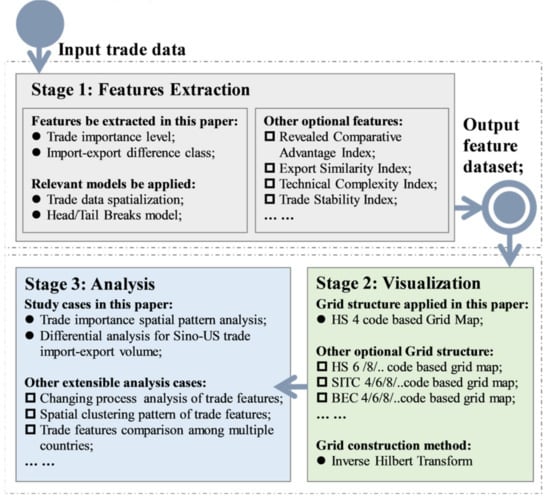
Figure 7. Extensible DTFM application framework.

Paths for developing DTFM theories, methods and applications can be summarized as two parts. On the one hand, a trade data specialization method can simultaneously express imports and exports of bilateral trade products with different periods. On that basis, it is interesting to develop a path tracking method to describe the various characteristics of trade relations, identify product types with drastic change and, thereby, explore the driving factors of mutation in bilateral trade. On the other hand, DTFM can express the static features of numerous types of products, and the spatial visualization process is unrestricted by the number of product types. In the next step, relevant works could focus on developing a coupling model to analyze the dynamic interactions of trade flows among multiple countries or groups.

5. Conclusions

The trade space has many features similar to geographical space, such as abstract expression of elements, space coordinates, spatial correlation and spatiotemporal variation. We believe that these features are of great significance in studying the trade structures and relations of numerous types of products. These features are difficult to express and analyze when traditional statistical methods or complex network methods are used.

In this paper, we proposed a new DTFM method for the visualization of bilateral trade features from a spatial perspective. The implementation process of DTFM can be summarized as feature extraction (Stage 1), visualization (Stage 2), and analysis (Stage 3). The China–US bilateral trade data were used in case studies. In Stage 1, ‘trade space’ was constructed using product imports and exports as the coordinate axis. Each type of product can be spatially transformed to a points set and expressed in the ‘trade space’ according to its annual imports and exports. Next, the trade features, including importance level and import–export difference class, were evaluated by spatial statistics and the head/tail breaks method. In Stage 2, a grid map was generated by the reverse application of the Hilbert curve generation method for visualization of the trade features. In Stage 3, the spatial pattern of the trade features was analyzed. In this way, bilateral trade features of plentiful different types of products are expressed with the advantages of clear expression, easy operationalization, good comparability, and high extensibility. Trade features aggregation characteristics of different products can also be expressed from a broader perspective. Furthermore, we propose an extensible DTFM application framework into which different trade features, different grid generation modes and numerous spatial analysis models can be readily integrated. In the future, we should develop methods for spatially understanding international trade systems.

References

- Boschma, R.; Capone, G. Relatedness and diversification in the European Union (EU-27) and European Neighbourhood Policy countries. Environ. Plan. C 2016, 34, 617–637. [Google Scholar] [CrossRef]
- Balassa, B. Trade liberalization and revealed comparative advantage. Manch. Sch. Econ. Soc. Stud. 1965, 33, 99–123. [Google Scholar] [CrossRef]
- Casanova, C.; Xia, L.; Ferreira, R. Measuring Latin America’s export dependency on China. JCEFTS 2016, 9, 213–233. [Google Scholar] [CrossRef]
- Dingemans, A.; Ross, C. Free trade agreements in Latin America since 1990: An evaluation of export diversification. CEPAL Rev. 2012, 108, 27–48. [Google Scholar] [CrossRef]
- Haddou, A.; Young, J. Comparative Intra-industry trade analysis on the asymmetric effects of the FTA: Korea and MENA Countries. J. Int. Trade Commer. 2018, 14, 49–62. [Google Scholar] [CrossRef]
- Cristelli, M.; Tacchella, A.; Gabrielli, A.; Pietronero, L.; Scala, A.; Caldarelli, G. Competitors’ communities and taxonomy of products according to export fluxes. EPJST 2012, 212, 115–120. [Google Scholar] [CrossRef]
- Ermann, L.; Shepelyansky, D. Ecological analysis of world trade. Phys. Lett. A 2013, 377, 3–4. [Google Scholar] [CrossRef][Green Version]
- Ermann, L.; Shepelyansky, D. Google matrix analysis of the multiproduct world trade network. EPJB 2015, 88, 84. [Google Scholar] [CrossRef]
- Dong, C.; Yin, Q.; Lane, K.; Yan, Z.; Shi, T.; Liu, Y.; Bell, M.L. Competition and transmission evolution of global food trade: A case study of wheat. Phys. A 2018, 509, 998–1008. [Google Scholar] [CrossRef]
- Basso, F.; Geciane, P.; Kannebley, J. International Trade Relations of Products for Wind Energy Production: A Study from the Dynamic Social Network Analysis (DSNA). In Proceedings of the 2017 Portland International Conference on Management of Engineering and Technology, Portland, OR, USA, 9–13 July 2017; pp. 1–18. [Google Scholar]
- Fu, X.; Yang, Y.; Dong, W.; Wang, C.; Liu, Y. Spatial structure, inequality and trading community of renewable energy networks: A comparative study of solar and hydro energy product trades. Energy Policy 2017, 106, 22–31. [Google Scholar] [CrossRef]
- Hao, X.; An, H.; Sun, X.; Zhong, W. The import competition relationship and intensity in the international iron ore trade: From network perspective. Resour. Policy 2018, 57, 45–54. [Google Scholar] [CrossRef]
- Pappalardo, G.; Allegra, V.; Zarba, A. The effects of the bsec on regional trade flows of agri-food products. In Proceedings of the SGEM 2014 Scientific Subconference on Political Sciences, Law, Finance, Economics and Tourism, Sofia, Bulgaria, 3–9 September 2014; Volume 4. [Google Scholar]
- Kivel, M.; Arenas, A.; Barthelemy, M.; Gleeson, J.; Moreno, Y.; Porter, M. Multilayer networks. J. Complex Netw. 2014, 2, 203–271. [Google Scholar] [CrossRef]
- Liu, X.; Stanley, H.; Gao, J. Breakdown of interdependent directed networks. Proc. Natl. Acad. Sci. USA 2016, 113, 1138–1143. [Google Scholar] [CrossRef]
- Latapy, M.; Magnien, C.; Vecchio, N. Basic notions for the analysis of large two-mode networks. Soc. Netw. 2008, 30, 31–48. [Google Scholar] [CrossRef]
- Hidalgo, C.; Klinger, B.; Barabsi, A.; Hausmann, R. The product space conditions the development of nations. Science 2007, 317, 482–487. [Google Scholar] [CrossRef] [PubMed]
- Hidalgo, C.; Hausmann, R. The building blocks of economic complexity. Proc. Natl. Acad. Sci. USA 2009, 106, 10570–10575. [Google Scholar] [CrossRef] [PubMed]
- Vidmer, A.; Zeng, A.; Medo, M.; Zhang, Y.-C. Prediction in complex systems: The case of the international trade network. Phys. A 2015, 436, 188–199. [Google Scholar] [CrossRef]
- Mealy, P.; Farmer, J.; Teytelboym, A. Interpreting economic complexity. Sci. Adv. 2019, 51, 1705. [Google Scholar] [CrossRef]
- Hausmann, R.; Hidalgo, C. The Atlas of Economic Complexity: Mapping Paths to Prosperity; MIT Press Books; The MIT Press: Cambridge, UK, 2014; Volume 1. [Google Scholar]
- Fadeyi, O.; Bahta, T.; Ogundeji, A.; Willemse, B.J. Impacts of the SADC Free Trade Agreement on South African agricultural trade. Int. J. Entrep. Innov. 2014, 15, 53–59. [Google Scholar] [CrossRef]
- Mupela, E.; Szirmai, A. Communication costs and trade in sub Saharan Africa: A gravity approach. In e-Infrastructure and e-Services for Developing Countries. In AFRICOMM 2013. Lecture Notes of the Institute for Computer Sciences, Social Informatics and Telecommunications Engineering; Bissyandé, T., van Stam, G., Eds.; Springer: Cham, Switzerland, 2013; p. 135. [Google Scholar]
- Matkovski, B.; Radovanov, B.; Zekic, S. The effects of Foreign agri-food trade liberalization in South East Europe. Ekonomicky Casopis 2018, 66, 945–966. [Google Scholar]
- De, F.; De, S.; VIeira, J. Evaluation of logistic performance indexes of brazil in the international trade. RAM. Rev. Admin. Mackenzie 2015, 16, 213–235. [Google Scholar]
- Goodchild, M. Geographical information-science. IJGIS 1992, 6, 31–45. [Google Scholar] [CrossRef]
- Goodchild, M.; Haining, R.; Wise, S. Integrating GIS and spatial data analysis: Problems and possibilities. IJGIS 1992, 6, 407–423. [Google Scholar] [CrossRef]
- Goodchild, M.; Yuan, M.; Cova, T. Towards a general theory of geographic representation in GIS. IJGIS 2007, 21, 239–260. [Google Scholar] [CrossRef]
- Zipf, G.K. Human Behaviour and the Principles of Least Effort; AddisonWesley: Cambridge, MA, USA, 1949. [Google Scholar]
- Jiang, B.; Liu, X. Scaling of geographic space from the perspective of city and field blocks and using volunteered geographic information. IJGIS 2012, 26, 215–229. [Google Scholar] [CrossRef]
- Jiang, B. A topological pattern of urban street networks: Universality and peculiarity. Phys. A 2007, 384, 647–655. [Google Scholar] [CrossRef]
- Jiang, B. Street hierarchies: A minority of streets account for a majority of traffic flow. IJGIS 2009, 23, 1033–1048. [Google Scholar] [CrossRef]
- Fisher, W.D. On grouping for maximum homogeneity. J. ASA 1958, 53, 789–798. [Google Scholar] [CrossRef]
- Jenks, G.F. Generalization in statistical mapping. Ann. AAG 1963, 53, 15–26. [Google Scholar] [CrossRef]
- Wang, J.F.; Li, X.H.; Christakos, G.; Liao, Y.; Zhang, T.; Gu, X.; Zheng, X. Geographical detectors-based health risk assessment and its application in the neural tube defects study of the Heshun region, China. IJGIS 2010, 24, 107–127. [Google Scholar] [CrossRef]
- Jiang, B.; Ma, D. How complex is a fractal? Head/tail breaks and fractional hierarchy. J. Geovisualization Spat. Anal. 2018, 2, 1–6. [Google Scholar] [CrossRef]
- Jiang, B.; Yin, J. Ht-Index for quantifying the fractal or scaling structure of geographic features. Ann. AAG 2014, 104, 530–540. [Google Scholar] [CrossRef]
- Taleb, N.N. The Black Swan: The Impact of the Highly Improbable; Allen Lane: London, UK, 2007. [Google Scholar]
- Jiang, B. Head/Tail Breaks: A new classification scheme for data with a heavy-tailed distribution. Prof. Geogr. 2012, 65, 482–494. [Google Scholar] [CrossRef]
- Ye, S.J.; Zhang, C.; Wang, Y.; Liu, D.; Du, Z.; Zhu, D. Design and implementation of automatic orthorectification system based on GF-1 big data. TCSAE 2017, 33, 266–273. [Google Scholar]
- Ye, S.J. Research on application of Remote Sensing Tupu-take monitoring of meteorological disaster for example. AGCS 2018, 47, 892, (In Chinese with English abstract). [Google Scholar]
- Ye, S.; Liu, D.; Yao, X.; Tang, H.; Xiong, Q.; Zhuo, W.; Du, Z.; Huang, J.; Su, W.; Shen, S.; et al. RDCRMG: A raster dataset clean & reconstitution multi-grid architecture for remote sensing monitoring of vegetation dryness. Remote Sens. 2018, 10, 1376. [Google Scholar]
- Yao, X.; Mokbel, M.; AlArabi, L.; Eldawy, A.; Yang, J.; Yun, W.; Li, L.; Ye, S.; Zhu, D. Spatial coding-based approach for partitioning big spatial data in Hadoop. Comput. Geosci. 2017, 106, 60–67. [Google Scholar] [CrossRef]
- Ye, S.J.; Yan, T.L.; Yue, Y.-L.; Lin, W.-Y.; Li, L.; Yao, X.; Mu, Q.-Y.; Li, Y.-Q.; Zhu, D.-H. Developing a reversible rapid coordinate transformation model for the cylindrical projection. Comput. Geosci. 2016, 89, 44–56. [Google Scholar] [CrossRef]
- Wang, S.; Xu, X. A new algorithm of hilbert scanning matrix and its MATLAB program. J. Image Graph. 2006, 1, 119–122. [Google Scholar]
© 2020 by the authors. Licensee MDPI, Basel, Switzerland. This article is an open access article distributed under the terms and conditions of the Creative Commons Attribution (CC BY) license (http://creativecommons.org/licenses/by/4.0/).