The Spatial Heterogeneity of Factors of Drug Dealing: A Case Study from ZG, China

Abstract

Drug addiction and drug-related crime caused by drug dealing are serious problems for many countries. Such problems have gained urgency in China during recent years. However, there has been no research on the relationship between drug dealing and associated factors and its variation over space at a fine scale, such as the police station management area (PSMA), in China. Based on a seven-year data set obtained in ZG city, China, a geographically weighted Poisson regression (GWPR) model was employed to explore the spatial heterogeneity in the relationship between drug dealing and related risk factors, including social-demographic factors and environmental characteristics. The model results indicated that there were more drug dealings in the socially disorganized areas, typically associated with urban villages and floating population. Spatial accessibility had significant impacts on drug dealing. While the main road showed a negative effect, areas with more branch roads and bus stops tended to attract more drug dealings. Additionally, we found that these relationships were spatially nonstationary across space. This research represents the first in discerning spatial variation of drug dealing within a major Chinese city. These findings not only help policy makers better understand drug dealings from a geographical perspective, but can also help them to develop more targeted local intervention strategies.

1. Introduction

Approximately 275 million people around the world had at least one drug use experience during 2016, which accounts for 5.6% of the total population aged 15–64 [1]. The consequences of drug abuse are very serious, even depriving people of their lives. For example, 450,000 people died directly or indirectly from drug abuse in 2015 [1]. In addition, the economic cost of drug abuse is also high, for example, the annual expenditure for controlling drug abuse in the UK is as high as £15.7 billion [2]. Illegal drugs can also lead to other types of crimes, such as violence, general incivilities, and property crime [3,4]. Therefore, combating drug-related crimes, including drug dealing, is an important work of law enforcement departments in many countries.

In order to reduce the harm of drugs, law enforcement departments usually take legal actions to reduce the supply of drugs in hot spots of drug dealing. But this would lead to crime displacement, rather than fundamentally reducing the supply of drugs. Only by finding out the factors that affect the formation of the drug market and taking targeted measures can we fundamentally reduce the supply of drugs.

Drug dealing has been widely studied in many disciplines, including criminology, economics, sociology, and others. Some studies have explored the formation of hot spots in drug dealing from the perspective of the rational choice of drug dealers. The results show that drug dealers tend to choose places with high transaction volume and low risk. The results of studies on the hot spots of drug dealing show that there are often some locations with high levels of drug dealing [5,6,7,8], which may be related to locational characteristics that can facilitate drug trade. For example, a study conducted in New Jersey found that 46% of drug sales arrests occurred at 4.4% of all locations [9]. Identifying the characteristics of high-risk areas of drug dealing and allocating limited police resources to corresponding positions could effectively combat drug-related crimes.

To explore the relationship between drug dealing and risk factors, previous studies have employed traditional statistical models, such as multivariable regression [10], logistic regression [11,12], and risk terrain modeling have been employed to explore the relationship between drug dealing and risk factors [13,14,15]. Generalized lined model (GLM) is one of the most commonly used regression models to investigate the relationship between drug dealing and related factors when the dependent variable is the number of drug dealing crimes [16,17], which produces a set of global fixed coefficients across the study area. The assumption of GLM modeling is that the relationship between drug dealing and independent variables is stationary over space, which is not necessarily consistent with the truth.

The drug dealing crime data have been collected with geographical coordinates and spatial heterogeneity may arise in modeling such data. Spatial heterogeneity, so named by LeSage and Pace [18], means the relationship between variables changing over space. In other words, some factors may have greater impacts on the spatial pattern of drug dealing. Spatial heterogeneity could not be ignored in the process of spatial modeling, which could be addressed by geographically weighted regression (GWR). GWR, developed by Fotheringham and Brunson, offers a solution to explore the spatial variation relationship between dependent variables and explanatory variables [19]. Geographically weighted Poisson regression (GWPR) is the adaption of GWR when the dependent variable is a counting variable, such as the number of burglaries or homicides in crime analysis [20,21,22]. But as far as we know, GWPR has not been used for drug dealing analysis. Understanding the spatial variation relationship between drug dealing and related risk factors has clear policy implications, which may lead to a more targeted and appropriate response at the local scale, rather than a response to the whole region.

The main purpose of this research is to apply GWPR modeling in assessing the spatial pattern of drug dealing in a large Chinese city. Specifically, this study seeks to answer two research questions: (1) whether the relationship between drug dealing and its impact factors will change over space; (2) whether GWPR model is better than GLM models in analyzing drug dealing crimes. Such knowledgeable gain is not only conductive to academic progress, but also allows law enforcement departments to understand the geographical demand for their services, and then intervene to reduce the negative impact of drug dealing.

2. Study Area and Data

2.1. Study Area

After a series of crackdown campaigns, China began to experience the era of being drug-free for around thirty years, starting in the 1950s. However, the reform and open door policy from the 1980s, meant that drugs re-emerged in China. According to the World Drug Report, China has seized the most cocaine in Asia and the third largest amount of heroin in the world in 2006 [23]. The study area of this research is the main urban area of ZG city which located in the southeast of China. The premise of obtaining data from the public security department was that the real name of the city cannot be mentioned in publications, therefore the city was labeled ZG in this article. ZG city belongs to the province with the most serious drug-related crimes in China. The main urban area of ZG city covers an area of 1600km² with a total population about 9 million inhabitants.

2.2. Data Preparation

The drug dealing data were acquired from the Public Security Bureau of ZG city during the years 2012–2018 and a total of 10,301 drug dealing were recorded in the study area. As is shown in Figure 1, there are 85 drug dealings per police station management area (PSMA) on average during the study period ranging from 0 to 311. The social economic data and the demographic data were collected from the ZG statistical book [24]. Road and POI (Point of Interest) data were obtained from Guangdong RITU WANFANG technology Co. Ltd.

The crime risks have been explored at different spatially aggregated levels in previous studies, such as street segments, census tracts, and block groups, etc. Police station management areas (PSMAs) are now the only security-related division system in China which could be integrated with the public security management process easily. Compared with other administrative units, PSMAs are considered to have better homogeneity of public security management, since they are delineated by the local Public Security Bureau for security management. Therefore, PSMAs are employed as the spatial units for analysis in this study, which has been used in the analysis of burglary [20,25]. There are 122 PSMAs in the study area covering an area between 1 km² and 92 km², with an average of about 12 km².

The explanatory variables were selected according to crime theory and literature. Two dominant theories could be employed to explain the spatial distribution of drug dealing, namely social disorganization and rational choice.

Regarding social disorganization, high unemployment rate, low education level and high minority population are the typical characteristics of a socially disorganized community. These factors will make the community become a business-friendly area for drug dealing. These communities, with the lack of formal and informal guardianship, could not successfully fight against drug dealing. Three explanatory variables pertaining to this theory were selected, including urban village [26], floating population [21,25], and population with bachelor’s degree or higher (advanced degree) [27,28].

From the perspective of the rational choice theory, drug dealing is an illegal but commercial activity. Hence, drug dealers would aim to obtain high rewards, but low risks in terms of being caught by police. As a result, drug dealers would choose areas with more people and convenient transportation for drug trade. In this way, they can get as many customers as possible, and run away quickly in case of danger. As an important activity node, bus stops can increase the possibility of being a drug trading place from two aspects [4,13]. First, to serves as an anchor point of daily activities of drug users, it can attract drug addicts to particular areas. Second, bus stops can also attract drug users from other regions, and thus increase the number of potential drug transactions. The main road [16,29], branch road, and hotel [12] were also selected as the explanatory variables. All of the aforementioned variables were aggregated at the PSMA-level.

3. Methodology

GWPR is the main analysis method of this study, which could deal with the spatial nonstationary relationship between variables through the local regression coefficients. For the purpose of comparison, both GLM and GWPR were used to model drug dealing in this study. These two techniques and the measures for goodness of fit are described briefly in the following paragraphs. Spatial autocorrelation analysis with Moran’s I test and multicollinearity check between explanatory variables were conducted.

3.1. GLM

GLM models are the most commonly used crime modeling method. A GLM consists of three parts, including a random component, a systematic component and a link function component. According to the distribution of the dependent variable, the random component could be flexibly specified by the probability distribution, such as Poisson distribution or negative binominal distribution. Therefore, GLM has been widely used in crime analysis, since the count of crime usually obeys Poisson or negative binominal distribution [30,31,32]. The model form of GLM adopted in this study is as follows:

$$\ln \left({\mathrm{Y}}_{\mathrm{i}}\right)={\mathsf{\beta }}_0+{\mathsf{\beta }}_1\ln \left({\mathrm{P}}_{\mathrm{i}}\right)+{\mathsf{\beta }}_2{\mathrm{x}}_{\mathrm{i}2}+{\mathsf{\beta }}_3{\mathrm{x}}_{\mathrm{i}3}+\dots +{\mathsf{\beta }}_{\mathrm{k}}{\mathrm{x}}_{\mathrm{ik}}+{\mathsf{\epsilon }}_{\mathrm{i}}$$

(1)

where ${\mathrm{Y}}_{\mathrm{i}}$ is the expected number of drug dealings per PSMA, ${\mathrm{P}}_{\mathrm{i}}$ is the total population in $i$-th PSMA, ${\mathrm{x}}_{\mathrm{ij}}$ is the $j$-th explanatory variable, ${\mathsf{\beta }}_0,{\mathsf{\beta }}_1, \dots {\mathsf{\beta }}_{\mathrm{k}}$ are model parameters and ${\epsilon }_i$ is the $i$-th random error term. The coefficients $\mathsf{\beta }$ of explanatory variables in the above model do not change over PSMAs, which is the average impact of variable $j$ on drug dealings in the study area.

3.2. GWPR

The results of the above GLM are composed of a series of global fixed parameters, which could not account for the spatial heterogeneity in the relationship between dependent variables and independent variables. GWPR is a potential methodology to address this issue by allowing the coefficients to vary spatially. Regression coefficients are functions of geographical coordinates of each analysis unit. The form of GWPR model is presented below:

$$\ln \left({\mathrm{Y}}_{\mathrm{i}}\right)={\mathsf{\beta }}_0\left({\mathrm{u}}_{\mathrm{i}},{\mathrm{v}}_{\mathrm{i}}\right)+{\mathsf{\beta }}_1\left({\mathrm{u}}_{\mathrm{i}},{\mathrm{v}}_{\mathrm{i}}\right)\ln \left({\mathrm{P}}_{\mathrm{i}}\right)+{\displaystyle \sum }_{\mathrm{k}=2}^{\mathrm{p}}{\mathsf{\beta }}_{\mathrm{k}}\left({\mathrm{u}}_{\mathrm{i}},{\mathrm{v}}_{\mathrm{i}}\right){\mathrm{X}}_{\mathrm{ik}}+{\epsilon }_i$$

(2)

where $\left({\mathrm{u}}_{\mathrm{i}},{\mathrm{v}}_{\mathrm{i}}\right)$ is the geographic coordinate of the center point of $i$-th PSMA, ${\mathsf{\beta }}_{\mathrm{k}}$ is the function of $\left({\mathrm{u}}_{\mathrm{i}},{\mathrm{v}}_{\mathrm{i}}\right)$ varying across PSMAs, which could be estimated as follows:

$$\widehat{\mathsf{\beta }}\left({\mathrm{u}}_{\mathrm{i}},{\mathrm{v}}_{\mathrm{i}}\right)={\left({\mathrm{X}}^{\mathrm{T}}\mathrm{W}\left({\mathrm{u}}_{\mathrm{i}},{\mathrm{v}}_{\mathrm{i}}\right)\mathrm{X}\right)}^{-1}{\mathrm{X}}^{\mathrm{T}}\mathrm{W}\left({\mathrm{u}}_{\mathrm{i}},{\mathrm{v}}_{\mathrm{i}}\right)\mathrm{Y}$$

(3)

where $\mathrm{W}\left({\mathrm{u}}_{\mathrm{i}},{\mathrm{v}}_{\mathrm{i}}\right)$ is an $n$ by $n$ spatial weight matrix which can be described as:

$$\mathrm{W}\left({\mathrm{u}}_{\mathrm{i}},{\mathrm{v}}_{\mathrm{i}}\right)=\left[\begin{array}{cccc}{\mathrm{w}}_{i1}& 0& \dots & 0\\ 0& {\mathrm{w}}_{i2}& \dots & 0\\ \dots & \dots .& \dots & \dots \\ 0& \dots & \dots & {\mathrm{w}}_{in}\end{array}\right]$$

(4)

where the diagonal element $w_{in}$ is the weight given to PSMA $j$ in the calibrating process of model for PSMA $i$, while the off-diagonal elements are zero [33].

The regression equation of each PSMA is estimated by the observations in nearby PSMAs. Each PSMA is weighted according to its distance from the regression point. Hence, for a PSMA $i$, the closer the observations to it, the greater the impact on the estimation of $\widehat{\mathsf{\beta }}\left({\mathrm{u}}_{\mathrm{i}},{\mathrm{v}}_{\mathrm{i}}\right)$ and the magnitude of this effect is usually calculated by two weight functions as follows:

Gaussian:

$${\mathrm{w}}_{\mathrm{ij}}=\exp \left(-\frac{1}{2}\ast {\left(\frac{{\mathrm{d}}_{\mathrm{ij}}}{\mathrm{b}}\right)}^2\right)$$

(5)

Bi-square:

$${\mathrm{w}}_{\mathrm{ij}}=\{\begin{array}{c}{\left(1-\left(\frac{{\mathrm{d}}_{\mathrm{ij}}}{{\mathrm{b}}_{\mathrm{i}\left(\mathrm{k}\right)}}\right)\right)}^2\mathrm{if}f {\mathrm{d}}_{\mathrm{ij}}<{\mathrm{b}}_{\mathrm{i}\left(\mathrm{k}\right)}\\ 0 \mathrm{otherwise}\end{array}$$

(6)

where $d_{ij}$ is the distance between PSMA $i$ and $j$, $\mathrm{b}$ is the fixed bandwidth, ${\mathrm{b}}_{\mathrm{i}\left(\mathrm{k}\right)}$ is the adaptive bandwidth which is employed in this research.

The selection of optimal bandwidth is another important issue in GWPR modeling, which could be addressed by Akaike information criterion (AIC). AIC was also adopted to evaluate the performance of models. The model with the minimum AIC value is the optimal one.

The calibration of GWPR model was based on Tobler’s first law of geography: “everything is related to everything else, but near things are more related than distant things” [34]. Considering this issue, compared with the global model, GWR is more suitable for area-based crime modeling, because it could successfully capture the spatial heterogeneity between crime counts and explanatory variables.

3.3. Spatial Autocorrelation and Multicollinearity

Moran’s I is a measure of spatial autocorrelation proposed by Moran [35], which was employed in this research to investigate whether the residuals of the proposed models were correlated spatially among adjacent PSMAs. The Moran index varies from −1 to 1. A negative value means a negative spatial autocorrelation and vice versa.

Although multicollinearity does not affect the accuracy of model estimation, it does affect the significance test of some variables, which will introduce bias to model interpretation. Therefore, the bivariate correlation coefficients between explanatory variables were calculated to identify the highly correlated variables.

3.4. Measures of Goodness of Fit

In addition to AIC, the mean absolute deviation (MAD) was also used to measure the goodness of fit of the model which was described as follows:

$$\mathrm{MAD}=\frac{{{\displaystyle \sum }}_{\mathrm{i}=1}^{\mathrm{N}}\left|\widehat{{\mathrm{Y}}_{\mathrm{i}}}-{\mathrm{Y}}_{\mathrm{i}}\right|}{\mathrm{N}}$$

(7)

where ${\mathrm{Y}}_{\mathrm{i}}$ is the observed count of drug dealing in PSMA $i$, $\widehat{{\mathrm{Y}}_{\mathrm{i}}}$ is the predicted count of drug dealing in PSMA $i$, and N is the number of PSMA. The lower the value is, the better the fit of the model.

As the link function in GLM and its extensions GWPR is nonlinear, the aforementioned models could not produce $R^2$ or local $R^2$. Therefore, the deviation percentage explained by GLM and the local deviation percentage explained by GWPR were employed to evaluate the overall goodness of fit. The higher the local deviation percentage is explained, the better the fit of the model. GWPR and GLM were estimated by GWR 4.0 and Stata 12 separately.

4. Results

The descriptive statistics of explanatory variables and dependent variables are shown in

Table 1. Descriptive statistics of variables.

Variable	Description	Mean	S.D.	Min	Max
Dependent Variable
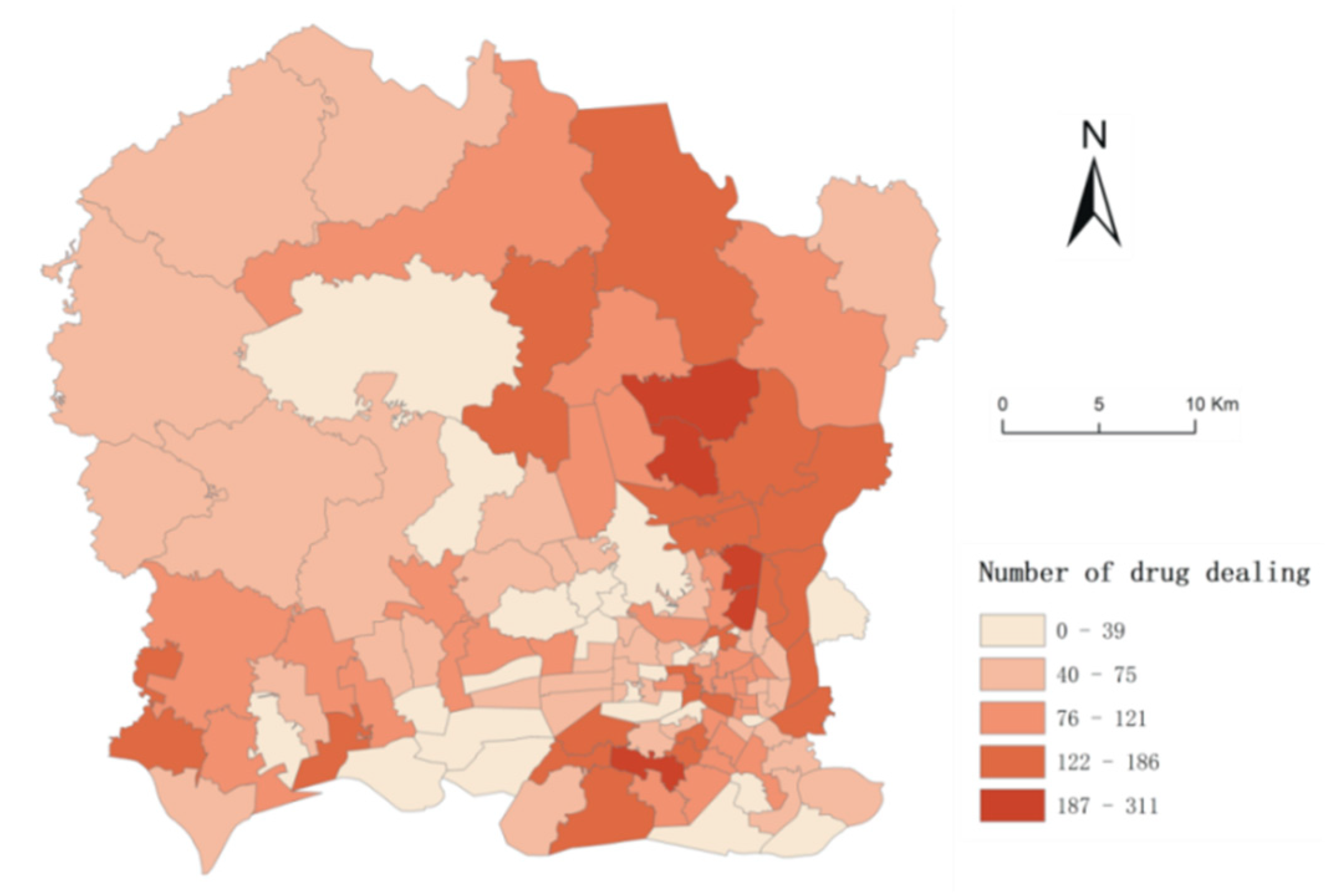
Drug dealing	Total number of drug dealings per PSMA	84.43	57.52	0	311
Explanatory variables
Urban village	The proportion of the total urban village area in each PSMA	5.57	6.21	0	24.29
HotelDen	The number of hotels per km2 in each PSMA	7.79	8.66	0	38.69
FloatingPOP	Percent of the number of people without local hukou in each PSMA (%)	37.92	21.19	0	87.28
BusStopDen	The number of bus stop per km2 in each PSMA	0.56	0.38	0	2.19
MainRoad	Percent of main road length (%)	3.23	3.24	0	17.92
BranchRoad	Percent of branch road length (%)	32.75	17.29	0	80.46
Advanced degree	Percent of people with a bachelor degree or higher in each PSMA	10.99	9.7	0	58.62

. The spatial distribution of drug dealing is presented in Figure 1. There there were spatial clusters formed in the east and southwest of the city (Moran’s I: Z-Score: 4.1168, p-value: 0.0000).

A bivariate correlation test was conducted before modeling and the results were presented in

Table 2. Bivariate correlation coefficient for explanatory variables.

	Urban village	HotelDen	FloatingPOP	BusStopDen	MainRoad	BranchRoad	Advanced Degree
Urban village	1
HotelDen	−0.435 *	1
FloatingPOP	0.662 *	−0.438 *	1
BusStopDen	−0.281 *	0.692 *	−0.312 *	1
MainRoad	−0.007	−0.156	0.163	−0.029	1
BranchRoad	0.581 *	−0.272 *	0.479 *	−0.274 *	−0.091	1
Advanced degree	−0.425 *	0.253 *	−0.334 *	0.118	0.058	−0.317 *	1

* for statistically significant at 0.05 confidence level.

. The correlation coefficients were less than 0.7, which means that there was no strong correlation between independent variables. Moreover, the variance inflation factor (VIF) was calculated for all independent variables. It is generally considered that multicollinearity among variables is acceptable if the VIF value is lower than 5. The largest VIF value was 2.348 (Urban village), which means that there is no risk of high multicollinearity between explanatory variables.

The GLM was used to model the relationship between drug dealing and related factors. Furthermore, the GWPR model was employed to account for the spatial relationship between the counts of drug dealing and explanatory variables. The results are presented in

Table 3. Estimation of GLM and GWPR models.

	GLM	GWPR
		Mean	Min	Lwr Quartile	Median	Upr Quartile	Max
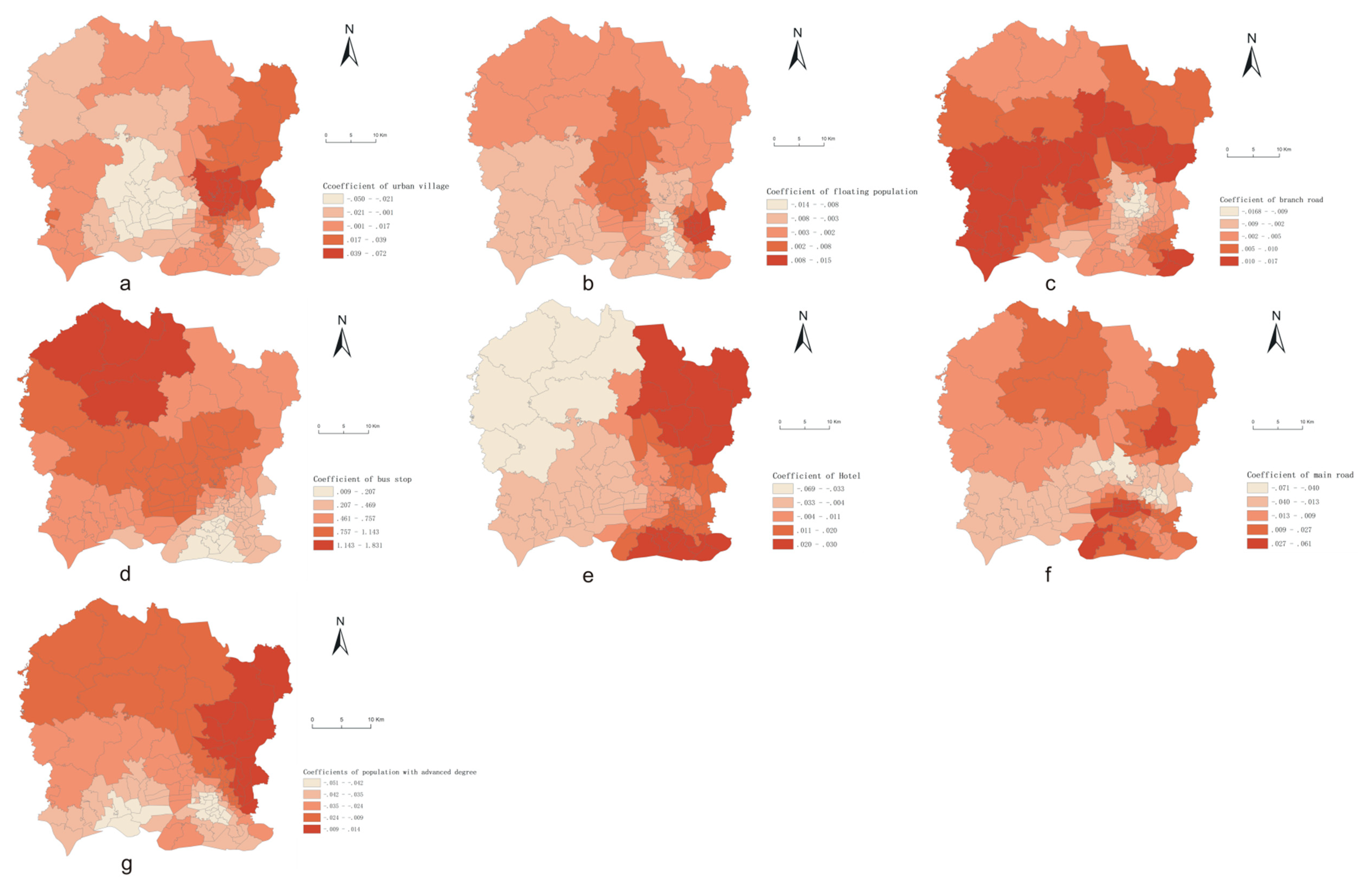
Urban village	0.007 *	0.0085	−0.0495	−0.008	0.0066	0.0213	0.0721
HotelDen	0.0134 *	0.0043	−0.0688	−0.0073	0.0099	0.0175	0.0304
FloatingPOP	0.0046 *	−0.0007	−0.0136	−0.0053	0.0009	0.0037	0.0155
BusStopDen	0.4687 *	0.5807	0.0089	0.2933	0.5228	0.8208	1.8311
MainRoad	−0.0074 *	−0.0025	−0.0714	−0.0193	−0.0019	0.0183	0.0606
BranchRoad	0.0059 *	0.0031	−0.0168	−0.0025	0.0032	0.0092	0.0168
Advanced degree	−0.0321 *	−0.0274	−0.0513	−0.0394	−0.0314	−0.0147	0.014
Intercept	−7.0477	−6.8879	−8.3962	−7.1453	−6.845	−6.5296	−5.8916
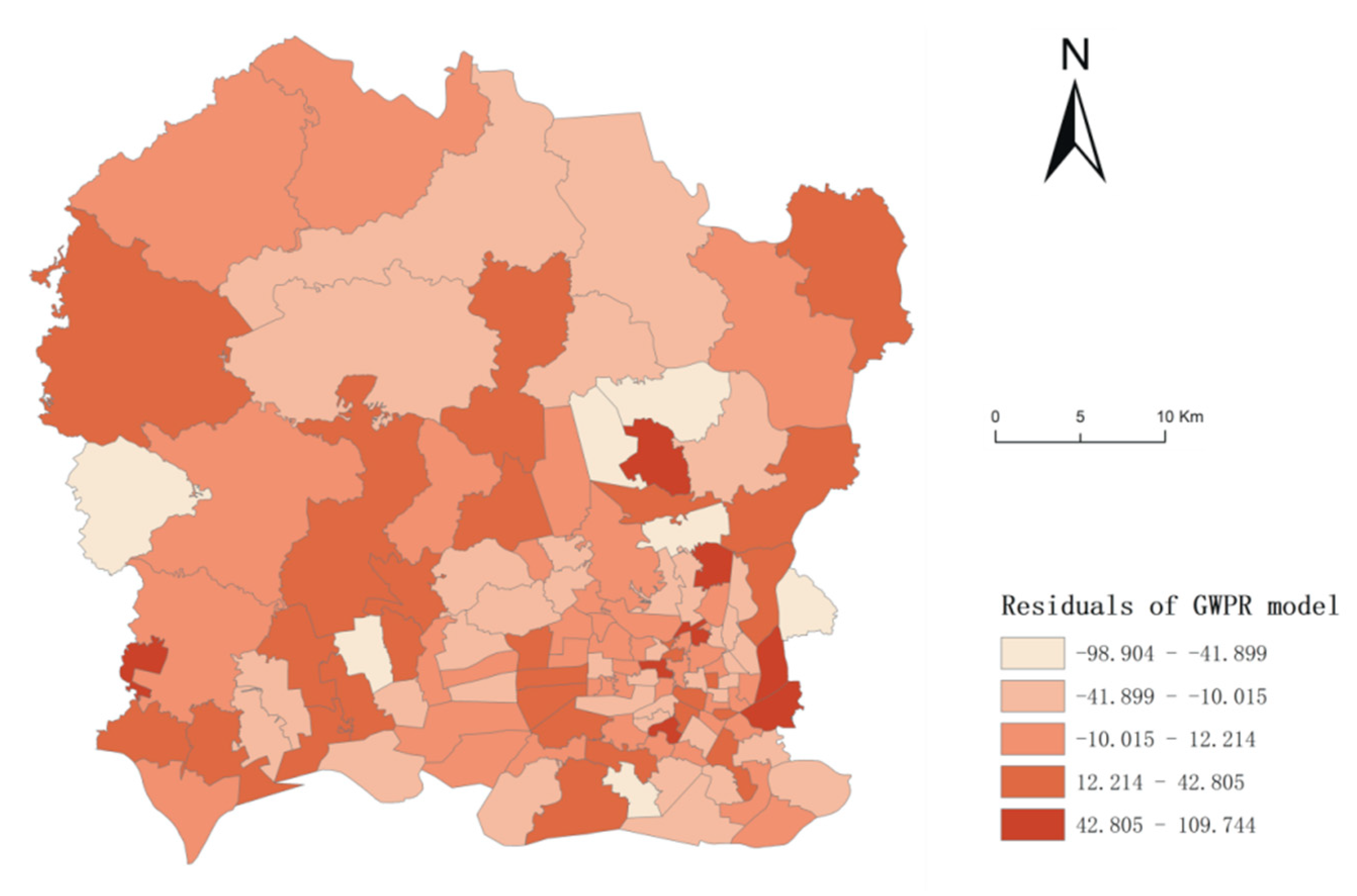
Moran’s I	0.162 *	−0.0286
MAD	26.5314	21.0873
Akaike’s Information Criterion (AIC)	1815.8540	1247.9778
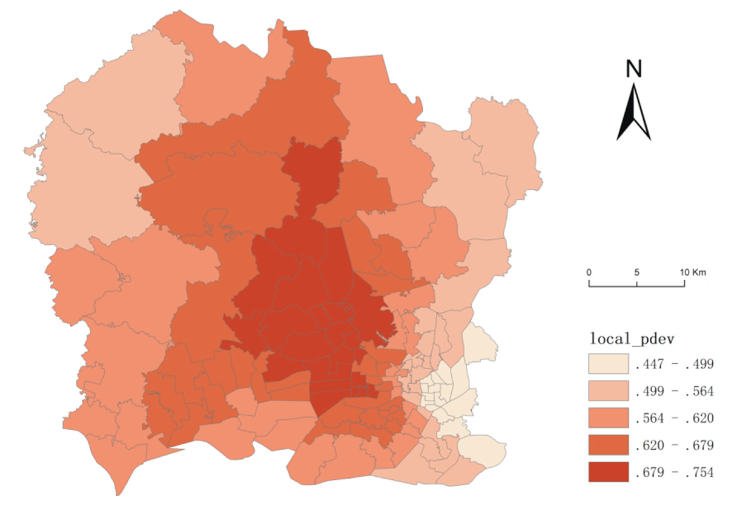
Percent deviance explained	0.445	0.638

* for Coefficients being statistically significant at 0.05 level.

. The coefficients of all explanatory variables in GLM are statistically significant and the signs are also in line with expectations. The main road and population, with advanced degree, has a negative impact on drug dealing, suggesting that with an increase in population with a bachelor degree or higher and a main road, the number of drug dealings decrease in each PSMA. On the other hand, the influence of other variables on drug dealings is positive, which means that, as these variables increase, so does the number of drug dealings.

Compared with GLM, GWPR could capture the spatial variation of the relationship between dependent and independent variables through local regression coefficients. The local parameters in GWPR are summarized in Table 3, which are presented as the minimum, lower quartile, median, upper quartile, and maximum. The coefficients of other variables range from negative to positive except for the coefficients of bus stop density, which are always positive.

The spatial patterns of model residuals are presented in Figure 2, suggesting no spatial autocorrelation (Moran’s I value: −0.0286, Z-Score: −1.142, p-value: 0.2536). Local percent deviance explained in GWPR is the counterpart to $R^2$ in a linear model, which indicates the spatial variation in explanatory power. The best fit of the model, as shown in Figure 3, is the center of the study area.

Four measures were used to compare the performance of the models above, Akaike’s Information Criterion (AIC), mean absolute deviance (MAD), percent of deviance explained, and the spatial correlation existing in the model residuals. Results shown in Table 3 revealed that GWPR outperformed GLM with a higher percent deviance explained, as well as lower AIC and MAD. The variability in drug dealings could be well captured by GWPR through accounting for the spatial heterogeneity.

The spatial agglomeration of crime has been widely documented in literature [20,21]. The underlying assumptions of the above models are that the error term is spatially independent. If the residual was spatial correlated, the model results would be biased [36]. The Moran’s I indices for model residuals were calculated to analyze the spatial autocorrelation and the results were presented in Table 3. It could be noted that the spatial correlation in the residuals of GLM was significant at 90% confidence level, whereas the residuals of GWPR do not appear to correlate spatially. This indicates that the spatial dependency of drug dealings has been fully addressed by the model.

5. Discussion

The advantage of GWPR over GLM is that it can account for spatial heterogeneity by allowing the parameters to vary spatially. Once the local parameters are obtained, they can be mapped and their spatial patterns could be explored. Therefore, we plotted the coefficients of each explanatory variable to exam its spatial pattern, and explore its possible causes, as many previous studies using GWPR models have done [2,22]. The application of GWPR to assessing drug dealings demonstrated the spatial variation of regression coefficients between the dependent variable and independent variables across PSMA areas in ZG city (Figure 4). The coefficients of urban village ranged from −0.05 to 0.72. The local t-statistics suggested that the urban village has a positive impact on drug dealing. Urban villages are usually associated with higher degrees of social disorganization, which are conducive to various criminal activities [37]. The complexity of the built environment, the diversity of the residents and the lack of social control in the urban village present challenges to fighting drug dealing. As illustrated in Figure 4a, the relationship between urban village and drug dealing is the strongest in the downtown areas. Compared with the peripheral areas, the formal and informal social control in the downtown areas of the city is stronger, which forces the drug dealers to confine their activities to the urban villages.

The coefficients of floating population ranged from −0.014 to 0.015. In previous studies, the impact of floating population on crime has been inconsistent. Some studies found that floating population had a positive impact on crime [38,39], but others had different findings [40]. For example, the impact of floating population on crime varies by the origins of the migrants [21]. The p-values confirmed that floating population has a positive impact on drug dealing. The spatial distribution of the coefficients (Figure 4b) demonstrated that the floating population had a greater influence in the city center than in the peripheral areas. The high residential mobility of a floating population is one of its important characteristics, because they usually have to move frequently to make a living. The increase of residential mobility would lead to an increase of property crime [41,42], whereas it had a negative impact on sex offenses [43]. The findings of this study showed that residential mobility had a positive effect on drug dealing.

As shown in Figure 4d, the coefficients of bus stop density were positive across the study area, which indicated that the increased number of of bus stops would increase the drug dealing. Similar results have been found in previous studies [13,14]. Although the local coefficients of bus stop density were positive in all PSMAs, the strength of this relationship is not constant. The effect of bus stops was the largest in the northwest, and gradually decreased towards the southeast. The areas with higher densities of bus stops are more accessible, providing affordable transportation for drug users to travel to drug dealing locations.

Hotels are considered to be one of the most important customer attractors in the drug sales market. There are more opportunities to meet potential drug buyers around the hotels. Therefore, hotels with poor management are often hot spots of illicit drug activities, which have a positive impact on drug-related crime [12,44]. As shown in Figure 4e, the influence of hotels in the downtown areas is lower than that in the suburbs, which may be due to the fact that there are many other suitable drug dealing places in the city center, such as restaurants, bars, and parks, etc. Coefficients in a few PSMAs were negative, and a local t-statistics test was carried out. The results suggested that the negative coefficients for most of the PSMAs (84.1%) are statistically insignificant.

Additionally, the sustainability of a drug market has much to do with its accessibility. Road network is an important indicator of accessibility. The road network determines the flow pattern of people and vehicles, which has been proven to be closely related to crime [45,46]. Some studies found that the impact of roading was negative [16], while others found it was positive [29,47]. Figure 4c,f were produced for branch roads and main roads respectively. The spatial distribution of coefficients of these variables were similar, both of which were negative in the central area and positive in the periphery. However, after checking the local t-value, we found that the negative coefficients of the branch road for most of the PSMAs (80.5%) were not significant at the 95% confidence level. Positive coefficients of the main road for a few PSMAs (16.9%) were significant. The possible explanation for this phenomenon is the crime reduction effects of CCTV (closed circuit television). CCTV has been proven to be an effective means of crime prevention [48,49]. However, limited by the financial budget, more cameras are installed along the main roads in downtown areas. Branch roads in periphery areas with fewer cameras are vulnerable to drug dealing.

Figure 4g shows the density of people with a bachelor degree or higher (Advanced degree), illustrating that there are strong negative trends in the population with advanced degree in most of the PSMAs, which suggest that increments in the population with advanced degrees contribute to the decrease in drug dealing. The relationship between education level and different types of crime has been widely explored in previous studies, such as burglary [20,50], homicide [22], and robbery [51,52]. The results of the above studies showed that the higher the proportion of people with advanced degrees (such as bachelor’s diploma or higher), the lower the number of crimes. Although previous research has found that the relationship between education level and drug abuse is not statistically significant [27], another study found a statistical relationship between education and the number of drug sales arrests, which was consistent with our findings [16].

From the above discussion, we found that the sign of the coefficients of most variables varied from negative to positive, except for bus stop density. This phenomenon is very common in the models based on GWR or its extensions and has been discussed in previous studies [53,54]. A possible explanation of this phenomenon is that although a bivariate correlation test has been carried out at the beginning of the model, it does not guarantee that there is no local multicollinearity among explanatory variables.

6. Conclusions

This study represents the first attempt in applying GWPR to discerning spatial variation of drug dealing within a major Chinese city. Drug dealing is a serious crime in many countries, as in China, because of its negative social impact, such as extensive economic cost and drug-related crimes. In order to fight against drug dealing, the related risk factors should be identified first. Based on a seven-year data set collected in a Chinese city ZG, this study explored the relationship between drug dealing and its influencing factors. The results indicated that when the number of urban villages and floating population increases, the number of drug dealings would increase. The relationship between roads and drug dealing does exist but varies across the city. Areas with more main roads experienced fewer drug dealings, whereas areas with more branch roads attracted more drug dealings. In addition, areas with higher densities of bus stops and hotels were linked to more drug dealings. The education level was negatively correlated with the number of drug dealings. Moreover, the results also indicated that the coefficients of the risk factors varied across the space.

The findings above not only help policy makers better understand drug dealings from a geographical perspective, but also help them to develop more targeted local intervention and prevention strategies. Localized strategies tend to be more effective than the traditional one-size-fits-all strategies, and they could reduce unnecessary expenditure of social resources.

This study has several limitations as well. First, according to the modifiable areal unit problem (MAUP) proposed by Openshaw [55], the results of spatial statistics are sensitive to the selected geographical unit. We could only get aggregated crime data at the PSMA level from the ZG police department at this time. Therefore, PSMA is the only geographical unit used in this research limited to the crime data. Future studies should employ data collected from different spatial scales. Second, this study only tested the relationship between drug dealing and related factors for a single city. Comparison studies across multiple cities are desirable to test the general applicability of the findings discovered in this research.

References

- UNODC. World Drug Report 2018; UN: New York, NY, USA, 2018. [Google Scholar] [CrossRef]
- Weir, R. Using geographically weighted regression to explore neighborhood-level predictors of domestic abuse in the UK. Trans. GIS 2019, 23, 1232–1250. [Google Scholar] [CrossRef]
- Braga, A.A.; Weisburd, D.L.; Waring, E.J.; Mazerolle, L.G.; Spelman, W.; Gajewski, F. Problem-oriented policing in violent crime places: A randomized controlled experiment. Criminology 1999, 37, 541–580. [Google Scholar] [CrossRef]
- Robinson, J.B.; Rengert, G.F. Illegal Drug Markets: The Geographic Perspective and Crime Propensity. West. Criminol. Rev. 2006, 7, 20–32. [Google Scholar]
- Weisburd, D.; Mazerolle, L.G. Crime and Disorder in Drug Hot Spots: Implications for Theory and Practice in Policing. Police Q. 2000, 2000. 3, 331–349. [Google Scholar] [CrossRef]
- Rengert, G.; Chakravorty, S.; Bole, T.; Henderson, K. A geographic analysis of illegal drug markets. Crime. Prev. Stud. 2000, 11, 219–239. [Google Scholar]
- Kennedy, L.W.; Caplan, J.M.; Piza, E. Risk Clusters, Hotspots, and Spatial Intelligence: Risk Terrain Modeling as an Algorithm for Police Resource Allocation Strategies. J. Quant. Criminol. 2011, 27, 339–362. [Google Scholar] [CrossRef]
- Taniguchi, T.A.; Ratcliffe, J.H.; Taylor, R.B. Gang Set Space, Drug Markets, and Crime around Drug Corners in Camden. J. Res. Crime Delinquency 2011, 48, 327–363. [Google Scholar] [CrossRef]
- Weisburd, D.; Green, L. Policing drug hot spots: The Jersey City drug market analysis experiment. Justice Q. 1995, 12, 711–735. [Google Scholar] [CrossRef]
- Eck, J. Preventing crime by controlling drug dealing on private rental property. Secur. J. 1998, 11, 37–43. [Google Scholar] [CrossRef]
- McCord, E.S.; Ratcliffe, J.H. A Micro-Spatial Analysis of the Demographic and Criminogenic Environment of Drug Markets in Philadelphia. Aust. N. Z. J. Criminol. 2007, 40, 43–63. [Google Scholar] [CrossRef]
- Bernasco, W.; Jacques, S. Where Do Dealers Solicit Customers and Sell Them Drugs? A Micro-Level Multiple Method Study. J. Contemp. Crim. Justice. 2015, 31, 376–408. [Google Scholar] [CrossRef]
- Barnum, J.D.; Campbell, W.L.; Trocchio, S.; Caplan, J.M.; Kennedy, L.W. Examining the Environmental Characteristics of Drug Dealing Locations. Crime Delinquency 2016, 63, 1731–1756. [Google Scholar] [CrossRef]
- Onat, I.; Akca, D.; Bastug, M.F. Risk Terrains of Illicit Drug Activities in Durham Region. Ontario. Can. J. Criminol. Crim. Justice 2018, 60, 1–29. [Google Scholar] [CrossRef]
- Escudero, J.A.; Ramírez, B. Risk terrain modeling for monitoring illicit drugs markets across Bogota, Colombia. Crime Sci. 2018, 7, 3. [Google Scholar] [CrossRef]
- Taniguchi, T.A.; Rengert, G.F.; McCord, E.S. Where Size Matters: Agglomeration Economies of Illegal Drug Markets in Philadelphia. Justice Q. 2009, 26, 670–694. [Google Scholar] [CrossRef]
- Johnson, L.T.; Taylor, R.B.; Ratcliffe, J.H. Need drugs, will travel? The distances to crime of illegal drug buyers. J. Crim. Justice 2013, 41, 178–187. [Google Scholar] [CrossRef]
- Lesage, J.P. Introduction to Spatial Econometrics; Chapman and Hall/CRC: New York, NY, USA, 2009. [Google Scholar]
- Fotheringham, A.; Brunsdon, C.; Charlton, M. Geographically Weighted Regression: The Analysis of Spatially Varying Relationships. 2002; John Wiley & Sons: Chichester, UK; Hoboken, NJ, USA, 2003. [Google Scholar]
- Chen, J.; Liu, L.; Zhou, S.; Xiao, L.; Song, G.; Ren, F. Modeling Spatial Effect in Residential Burglary: A Case Study from ZG City, China. ISPRS Int. J. Geo-Inf. 2017, 6, 138. [Google Scholar] [CrossRef]
- Chen, J.; Liu, L.; Zhou, S.; Xiao, L.; Jiang, C. Spatial Variation Relationship between Floating Population and Residential Burglary: A Case Study from ZG, China. ISPRS Int. J. Geo-Inf. 2017, 6, 246. [Google Scholar] [CrossRef]
- Sepúlveda Murillo, F.H.; Olmo, J.C.; de Cortázar, A.R.G. The spatial heterogeneity of factors of feminicide: The case of Antioquia-Colombia. Appl. Geogr. 2018, 92, 63–73. [Google Scholar] [CrossRef]
- UNODC. World Drug Report 2008; UN: New York, NY, USA, 2008. [Google Scholar] [CrossRef]
- China Statistics Bureau, China Statistical Yearbook; China Statistical Publishing House: Beijing, China, 2018.
- Chen, J.; Liu, L.; Xiao, L.; Xu, C.; Long, D. Integrative Analysis of Spatial Heterogeneity and Overdispersion of Crime with a Geographically Weighted Negative Binomial Model. ISPRS Int. J. Geo-Inf. 2020, 9, 60. [Google Scholar] [CrossRef]
- Liu, L.; Feng, J.; Ren, F.; Xiao, L. Examining the relationship between neighborhood environment and residential locations of juvenile and adult migrant burglars in China. Cities 2018, 82, 10–18. [Google Scholar] [CrossRef]
- Wooditch, A.; Lawton, B.; Taxman, F.S. The Geography of Drug Abuse Epidemiology Among Probationers in Baltimore. J. Drug Issues 2013, 43, 231–249. [Google Scholar] [CrossRef]
- Willits, D.; Broidy, L.M.; Denman, K. Schools and Drug Markets: Examining the Relationship Between Schools and Neighborhood Drug Crime. Youth Soc. 2013, 47, 634–658. [Google Scholar] [CrossRef]
- Andreas, M.S. Spatial Analysis of Crime Using Gis-Based Data: Weighted Spatial Adaptive Filtering and Chaotic Cellular Forecasting with Applications to Street-Level Drug Markets. Ph.D. Dissertation, Carnegie Mellon University, Schenley Park Pittsburgh, PA, USA, 1997. [Google Scholar]
- Liu, L.; Jiang, C.; Zhou, S.; Liu, K.; Du, F. Impact of public bus system on spatial burglary patterns in a Chinese urban context. Appl. Geogr. 2017, 89, 142–149. [Google Scholar] [CrossRef]
- Song, G.; Liu, L.; Bernasco, W.; Xiao, L.; Zhou, S.; Liao, W. Testing Indicators of Risk Populations for Theft from the Person across Space and Time: The Significance of Mobility and Outdoor Activity. Ann. Am. Assoc. Geogr. 2018, 108, 1370–1388. [Google Scholar] [CrossRef]
- Song, G.; Liu, L.; Bernasco, W.; Zhou, S.; Xiao, L.; Long, D. Theft from the person in urban China: assessing the diurnal effects of opportunity and social ecology. Habitat Int. 2018, 78, 13–20. [Google Scholar] [CrossRef]
- Fotheringham, A.S.; Charlton, M.E.; Brunsdon, C. Spatial Variations in School Performance: A Local Analysis Using Geographically Weighted Regression. Geogr. Environ. Model. 2001, 5, 43–66. [Google Scholar] [CrossRef]
- Tobler, W.R. A Computer Movie Simulating Urban Growth in the Detroit Region. Econ. Geogr. 1970, 46, 234–240. [Google Scholar] [CrossRef]
- Moran, P.A.P. Notes on continuous stochastic phenomena. Biometrika 1950, 37, 17–23. [Google Scholar] [CrossRef]
- Anselin, L. Spatial Econometrics: Methods and Models; Kluwer Academic Publisher: Dordrecht, The Netherlands, 1988. [Google Scholar]
- Zheng, S.; Long, F.; Fan, C.; Gu, Y. Urban Villages in China: A 2008 Survey of Migrant Settlements in Beijing. Eurasian Geogr. Econ. 2009, 50, 425–446. [Google Scholar] [CrossRef]
- Curran, D.J. Economic Reform, the Floating Population, and Crime: The Transformation of Social Control in China. J. Contemp. Crim. Justice 1998, 14, 262–280. [Google Scholar] [CrossRef]
- Situ, Y.; Liu, W. Transient Population, Crime, and Solution: The Chinese Experience. International Journal of Offender Ther. Comp. Criminol. 1996, 40, 293–299. [Google Scholar] [CrossRef]
- Zhao Shukai, A.K. Criminality and the Policing of Migrant Workers. China J. 2000, 43, 101–110. [Google Scholar] [CrossRef]
- Caminha, C.; Furtado, V.; Pequeno, T.H.C.; Ponte, C.; Melo, H.P.M.; Oliveira, E.A.; Andrade, J.S. Human mobility in large cities as a proxy for crime. PLOS ONE 2017, 12, e0171609. [Google Scholar] [CrossRef]
- Mburu, L.; Helbich, M. Crime Risk Estimation with a Commuter- Harmonized Ambient Population. Ann. Am. Assoc. Geogr. 2016, 106, 1–15. [Google Scholar] [CrossRef]
- Konkel, R.; Hafemeister, A.; Daigle, L. The Effects of Risky Places, Motivated Offenders, and Social Disorganization on Sexual Victimization: A Microgeographic- and Neighborhood-Level Examination. J. Interpers. Violence 2019. [Google Scholar] [CrossRef]
- Feng, J.; Liu, L.; Long, D.; Liao, W. An Examination of Spatial Differences between Migrant and Native Offenders in Committing Violent Crimes in a Large Chinese City. ISPRS Int. J. Geo-Inf. 2019, 8, 119. [Google Scholar] [CrossRef]
- Davies, T.; Johnson, S.D. Examining the Relationship Between Road Structure and Burglary Risk Via Quantitative Network Analysis. J. Quant. Crim. 2015, 31, 481–507. [Google Scholar] [CrossRef]
- Xiao, L.; Liu, L.; Song, G.; Ruiter, S.; Zhou, S. Journey-to-Crime Distances of Residential Burglars in China Disentangled: Origin and Destination Effects. ISPRS Int. J. Geo-Inf. 2018, 7, 325. [Google Scholar] [CrossRef]
- Eck, J. Drug Markets and Drug Places: A case control study of the spatial structure of illicit drug dealing. Ph.D. Dissertation, University of Maryland, College Park, MD, USA, 1994. [Google Scholar]
- Lim, H.; Wilcox, P. Crime-Reduction Effects of Open-street CCTV: Conditionality Considerations. Justice Q. 2017, 34, 597–626. [Google Scholar] [CrossRef]
- Piza, E.L. The crime prevention effect of CCTV in public places: a propensity score analysis. J. Crim. Justice 2018, 41, 14–30. [Google Scholar] [CrossRef]
- Du, F.; Liu, L.; Jiang, C.; Long, D.; Lan, M. Discerning the Effects of Rural to Urban Migrants on Burglaries in ZG City with Structural Equation Modeling. Sustainability 2019, 11, 561. [Google Scholar] [CrossRef]
- Long, D.; Liu, L.; Feng, J.; Zhou, S.; Jing, F. Assessing the Influence of Prior on Subsequent Street Robbery Location Choices: A Case Study in ZG City, China. Sustainability 2018, 10, 1818. [Google Scholar] [CrossRef]
- Zhou, H.; Liu, L.; Lan, M.; Yang, B.; Wang, Z. Assessing the Impact of Nightlight Gradients on Street Robbery and Burglary in Cincinnati of Ohio State, USA. Rem. Sens. 2019, 11, 1958. [Google Scholar] [CrossRef]
- Hadayeghi, A.; Shalaby, A.S.; Persaud, B.N. Development of planning level transportation safety tools using Geographically Weighted Poisson Regression. Accid. Anal. Prev. 2010, 42, 676–688. [Google Scholar] [CrossRef]
- Xu, P.; Huang, H. Modeling crash spatial heterogeneity: Random parameter versus geographically weighting. Accid. Anal. Prev. 2015, 75, 16–25. [Google Scholar] [CrossRef]
- Openshaw, S. The modifiable areal unit problem, in Quantitative Geography: A British View; Wrigley, N., Bennett, R.J., Wrigley, N., Bennett, R.J., Eds.; Routledge & Kegan Paul: London, UK, 1981; pp. 60–69. [Google Scholar]