Abstract
Recent developments in web map applications have widely affected how background maps are rendered. Raster tiles are currently considered as a regular solution, while the use of vector tiles is becoming more widespread. This article describes an experiment to test both raster and vector tile methods. The concept behind raster tiles is based on pre-generating an original dataset including a customized symbology and style. All tiles are generated according to a standardized scheme. This method has a few disadvantages: if any change in the dataset is required, the entire tile-generating process must be redone. Vector tiles manipulate vector objects. Only vector geometry is stored on the server, while symbology, rendering, and defining zoom levels run on the client-side. This method simplifies changing symbology or topology. Based on eight pilot studies, performance testing on loading time, data size, and the number of requests were performed. The observed results provide a comprehensive comparison according to specific interactions. More data, but only one or two tiles, were downloaded for vector tiles in zoom and move interactions, while 40 tiles were downloaded for raster tiles for the same interactions. Generally, the WebP format downloaded about three times fewer data than Portable Network Graphics (PNG).
1. Introduction
The first web map was presented by Xerox in 1993 [1]. It was only a single image, and to interact with the map, an entirely new image with the desired viewport range had to be loaded. This principle was used until Google introduced “slippy map” in 2005 [2], a new technology that made maps more accessible and load more quickly. Its principle was segmenting a map image into separate, smaller sections. The map was no longer a single image, but several images joined together seamlessly. Interaction with the map only required necessary sections of the map to be loaded and displayed, not the entire image. The images were called raster tiles, and all major map applications and software libraries adopted Google’s method.
Web applications have seen major changes since 2005, although tiled web map technology is still used in almost identical form. Tile formats have been experimented with to generate tiles on demand and change the size and resolution of the tiles, however, the methods have not seen any major changes since. Today’s user requirements are very different to the requirements of 14 years ago. Today, maps require dynamic, fluid, fast, and interactive properties. A potential solution is vector tiles, which still employ the principle of dividing maps into squares, but instead of images, vector objects are loaded. All of the objects on a map can then be manipulated using JavaScript, can be queried, their symbology can be changed, and much more. While raster-based applications are the de facto standard today, vector tiles are becoming a more popular solution. Major web mapping services such as Google Maps and Mapbox, for example, have begun the migration from raster tiles to vector technology, though many other map services still rely on raster tiles, typically in satellite or aerial basemaps (including worldwide and well known portals such as Bing Maps, ArcGIS Online, mapy.cz, etc.), many derived from OpenStreetMap (e.g., Mapnik, Stamen, Positron, OpenTopoMap, etc.), basemap layers by Esri (WorldStreetMap, DeLorme, WorldTopoMap, etc.), national and regional map services (e.g., Czech Cadastral Office), or custom generated data for local purposes. Leaflet Providers [3] gives an overview of dozens of raster basemaps.
This work compares the performance of raster and vector tiles. The main aim of the experiment was to compare different load metrics focusing on the server-end and network testing. Testing was conducted using eight pilot studies to measure the application performance on four measurable metrics and one non-measurable metric. The study seeks to answer whether loading vector tiles is quicker than raster ones, and if any difference in performance is a result of the selected method. Performance testing and the results obtained enabled a comprehensive comparison of the methods from both the theoretical and practical points of view. The results may assist developers in their choice of applying raster or vector tile map methods to applications.
2. Map Tiles
Goodchild [4] mentioned the concept of map tiles when web maps were seldom applied. Tiles were compared to a system of tourist maps that only showed selected areas on a large-scale map sheet. Each additional area was located on a different sheet, and if users needed to combine maps to create a map with a larger area, they had to place the sheets side by side. This system is very similar to today’s map tile technology. Web map development began after 1993, when placing images on the web became possible [5]. The first web maps were generally only scanned images that were uploaded to a server. A user-generated interactive map was created for the first time in 1993 at the Xerox Palo Alto Research Center [1], though the map was re-generated each time the server was queried. This technology was also applied in MapQuest’s Web Map, which was the most popular Web Map from 1996 to 2009 [5]. In 2005, Google introduced Google Maps based on slippy map technology. This consisted of generating map tiles in advance, and only pre-generated tiles were displayed at the user’s request, and not the entire map. Zooming on the map only downloaded tiles other than those initially displayed. This technology has since been adopted by most web map services [2]. Sample et al. [1], Jiang et al. [6], and Veenendaal et al. [7] have described the current status of geoportals and basemaps. Zalipnys [8] or Villar-Cano et al. [9] conducted case studies on raster tile implementation, while Xiaochuang [10], Wan et al. [11], Zouhar et al. [12], or Li et al. [13] illustrated case studies on vector data in combination with big data.
2.1. Raster Tiles
To create raster tile maps, the required area must be divided into sections. Users generally do not perceive how data are stored when map tile layers are loaded for viewing from different services as these differences happen in the background. Each tile set has a defined data storage scheme. Yang et al. [14] described schemes as having several parameters such as pixel size, tile shape and size, coordinate system origin, tile matrix size, and number of zoom levels.
Stefanakis [15] also mentioned the map coordinate system as an important parameter. Almost all web maps today use the Web Mercator coordinate system (EPSG: 3857) [16], which was created by Google and modified the original Mercator projection system. Under this coordinate system, the world map can be displayed as a square by removing the polar regions. This square is a key feature in tile maps and is used as a zero zoom-level tile. Each additional zoom level is created by dividing the previous tile into four new tiles. The main difference between individual schemes is their coordinate system origin and tile numbering. Google names its tiles with a pair of X and Y coordinates (Figure 1a). To obtain a selected tile, its coordinates and zoom level must also be known, since each additional zoom level begins with a tile with coordinates 0,0. Numbering begins from the upper left corner. The second most commonly used tile numbering system (implemented, for example, by Bing Maps; Figure 1b) also places the origin at this point, but uses the Quadtree algorithm to name each tile. Each new zoom level keeps the tile number and adds a number from 0–3 to the next position. The tile in the first zoom level is indicated as 0, and the four tiles in the next zoom level are indicated as 00, 01, 02, and 03. [1]. The Open Geospatial Consortium (OGC) defines the Web Map Tile Service (WMTS) standard for raster tiles [17].
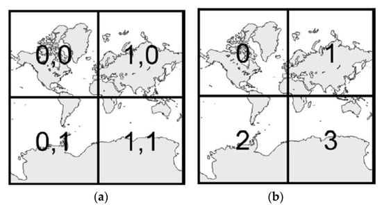
Figure 1.
Scheme of Google map tiles (a) and Bing map tiles (b).
Zavadil [18] wrote that web services most often use a tile size of 256 × 256 pixels. Less common tile sizes of 64 × 64 and 512 × 512 pixels are also in use [1]. Peterson [19] estimated the average memory requirement to store a single map tile of 256 × 256 pixels at 15 kB. The total number of tiles using 20 zoom levels is about one trillion, which is approximately 20,480 TB of data [6]. Raster tiles must be generated for each zoom separately, and the number of tiles increases by a factor of four at each zoom level.
A technique permitting server-side map generation that saves the results for future use (not directly after receiving a query) is known as a cache. Web servers can then immediately pass the results to clients without requiring servers to perform the requested action. A cache reduces demand on the Geographical Information System (GIS) and database servers and enables quicker map work. Caches are usually created for maps that do not change frequently (street networks, orthophotos, altimetry maps), while for frequently changing maps, the cache is updated regularly. Caches can also be created for browsers to allow content that has already been downloaded from the server to be re-used without downloading the content again, thereby reducing server footprint and improving Internet speed [20].
The raster tile symbology is created before the tiles are generated. Any modifications to symbols require that the entire tile set to be regenerated, which is one of the main disadvantages of raster map tiles. If assets are provided as WMTS, users can define a custom symbology in order to render with GetMap. This is accomplished using a standardized styled layer descriptor (SLD) and symbology encoding (SE) services by creating a document in XML format through which displayed layers can be paired with the symbology described in the document according to the symbology encoding standard.
2.2. Vector Tiles
Although raster tile maps were a revolutionary idea at the beginning of the twenty-first century, it now has many disadvantages, typically due to the need to generate an entire set of tiles each time the data geometry or symbology changes. Raster tile maps also do not permit users to interact with web maps [21].
Vector tile maps are more recent than raster tiles and were pioneered by Google, which implemented them in 2010 in the mobile version of Google Maps, and then again in the web version in 2013 [22]. Generally, vector tiles do not display images, but are vector objects stored on the server side displayed to the client. Vector data are only points, lines, and polygons represented by their vertex points and do not contain any information for rendering.
The vector tile pattern is the same as the raster tile pattern and divides the original vector dataset into a tiling grid (Figure 2), each corresponding to the data displayed on the tile. If a vector object belongs to more tiles, the object is divided, and each section is displayed on a different tile. The client displays only the data in its area of interest. Figure 2 illustrates the tile generation process according to Gaffuri [23].
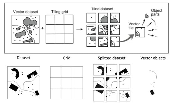
Figure 2.
The process of generating vector tiles (according to Gaffuri [23]).
Like raster tiles, only the data required by the client are transmitted after separating the dataset into tiles. Tiles must also be named according to a specific scheme. Most vector tile applications use the Google XYZ scheme [24]. Vector tiles are numbered in exactly the same manner as raster equivalents. For example, at a zoom level of 4 in column 8 and line 4, a tile would be numbered 4/8/4.png for the raster and 4/8/4.geojson for the vector. While vector tiles allow a progressive (decimal) increase in the zoom level (e.g., zoom 8.5), raster tiles are generated only for each incremental zoom level (e.g., zoom 8 or 9, etc.).
According to Netek et al. [25], the most commonly used formats are GeoJSON, TopoJSON, and Mapbox Vector Tile (mvt). The GeoJSON format is based on JSON (JavaScript Object Notation), which is a universal data format, and stores data as points, lines, polygons, multipoints, multilines, multipolygons, and geometric collections [26]. It has a simple structure and is independent of the platform in use. TopoJSON is a topological extension of GeoJSON and stores the geometry for all objects together, not separately. This reduces the amount of data since each part of the geometry is saved only once and each object refers to the geometry. Data size can be reduced by up to 80% in this manner [27].
Mapbox Vector Tile is an open format based on Google Proto[col Buffers, which is a language and platform-independent mechanism for serializing structured data [28]. Tiles are arranged according to the Google scheme using the Web Mercator coordinate system (EPSG: 3857). In 2015, Esri also announced support for Mapbox Vector Tile [29]. Each object’s geometry is stored relative to the origin of each tile. Objects can possess the following geometry: Unknown, Point, MultiPoint, LineString, MultiLineString, Polygon, or MultiPolygon.
Changing symbology is a major advantage of vector tiles. Compared to raster tiles, the client may request changes in the style of vector data displayed on a map. A style always includes a reference to the data to be rendered and rules for rendering. Several standards and specifications define how a symbology is created and subsequently applied in map data:
- Mapbox GL Styles – Open standard for other services. Created as a symbology into mvt format by Mapbox. The style is stored as a JSON object with specific root elements and properties [30]. Symbology is edited with visual editors (Mapbox Studio Style Editor; Maputnik) or by editing the JSON file.
- CartoCSS – Developed by Mapbox in 2010 as the predecessor of Mapbox GL Styles. It is very similar to Cascading Style Sheets (CSS) for web pages. Currently used by TileMill, Carto.
- Geo Style Sheets – One of the first specifications, used in the Cartagen project. Similar to CSS, but never established in major libraries.
- MapCSS – Open specification used to style data from OpenStreetMap (OSM), also based on CSS. It uses tags (strictly) from OSM.
3. Deployment of the Pilot Studies
3.1. Data and Front-End Interface
The pilot studies demonstrated the potential use of map data as either raster or vector tiles. All of the map applications (at the front-end) used the Mapbox GL JS library. Currently (12/2019), only three map libraries fully support the visualization of both vector and raster tiles: OpenLayers v3, Mapbox GL, and ArcGIS API for JS by Esri. While Esri’s solution is more complicated to implement and may have some legal restrictions under its academic license, OpenLayers and Mapbox are comparable. The authors used Mapbox because of its better documentation, but otherwise, the User Interface (UI) and datasets of all the applications were the same (Figure 3). The front-end interface contained basic map controls (zoom in/out, orientation and full screen buttons) at the top right, a menu with four items for the four interactive steps (see Section 4.1) at the top left, a scale at the bottom right, and a current zoom-level indicator. The back-end technology and data storage, however, were significantly different. The dataset contained three layers: a layer of tiles for the Czech Republic from the OpenMapTiles (OMT) project [30], a layer for the municipal borders of the Czech Republic, and an airport layer (source OpenStreetMap). Data were selected in order to cover the extent of all three levels: national (OMT), regional (borders), and local (airports). Eight applications were created (Table 1). Three different server data storage hosts were used (Mapbox Studio web application hosting, Wedos commercial hosting, Amazon Web Services EC2 Cloud). Raster tiles were created in two different file formats (PNG and WebP). Two of the raster tile applications used pre-generated tiles stored by the host, the other two applications generated raster tiles from vector data on request.
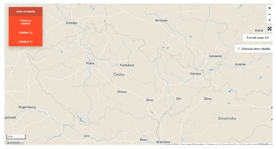
Figure 3.
Front-end interface of the pilot studies.

Table 1.
Overview of the pilot studies.
3.2. Pilot Study Based on Mapbox Studio
Mapbox Studio [31] is a web application for creating maps using either vector or raster tiles and uses the new Mapbox GL Styles open standard for mapping styles. Mapbox Studio has three sections: Styles, Tilesets (a collection of vector or raster tiles), and Datasets (a collection of features and their attributes). Basic default map data are also available from Mapbox. To use a custom dataset, creating or uploading data in one of the supported formats is possible. These data are then saved as a Tileset after editing. Once the data are uploaded, map styling is applied (Styles). The style is created according to the Mapbox GL styles specification. Table parameters can be edited through a graphical interface or by editing the JSON configuration file (style.json) [32], and the style obtains a unique ID in the format “user.ID”. The web map application uses Mapbox GL JS technology [33], and maps are initialized by assigning the object “mapboxgl.Map” to the variable “var map”. Attributes then specify the style ID and access key.
In this pilot study, three data layers were uploaded as a Tileset: a set of tiles for the Czech Republic from the OpenMapTiles project in MBTiles format, an airport data layer in the GeoJSON format, and a border layer in the GeoJSON format. A Klokantech Basic Style was applied to the pilot study, and finally, a configuration file was created and assigned a defined style (stored in Mapbox internal storage: mapbox://styles/francimor94/cjs5xhdis1zvj1glmsfnhqaax).
3.3. Pilot Studies Based on TileServer GL
TileServer GL [34] is a server application for rendering both vector and raster tiles, written in JavaScript and runs in Node.js. TileServer GL can be used for deployment on a localhost as a Docker container, although TileServer GL is commonly used as a server or cloud application. As well as rendering and tile services in advance, TileServer GL provides tile generation on request. TileServer GL is configured in the config.json configuration file, which defines the style, font, and data directories. Tiles are named and stored according to Google Scheme (see Section 2.1), and to access tiles in a map application, the “tiles” parameter contains the full URL path ending in “{z}/{x}/{y}.png” or “{z}/{x}/{y}.webp”. Due to the character of raster tiles, changing the style successively is not possible and any change to the style requires the entire set of tiles to be re-generated.
Three of the pilot studies used the open source TileServer GL from Klokan Technologies. The first pilot study used pre-generated vector tiles in the MBTiles format, while the other two pilot studies covered on-request rendering of raster tiles and created PNG and WebP raster tiles. The tiles were rendered at a resolution of 256 × 256 pixels with a 32-bit color depth and 0–14 zoom levels.
In these studies, the Maputnik [35] web editor was used to define the map style. The Klokantech Basic Style file was saved in the same folder as the server source files and map data, and the URL parameter for each resource was not populated with the precise URL, instead with the string “mbtiles://{resource ID}”. Amazon EC2 cloud storage [36] was used, with the following specifications: Intel Xeon 2.5 GHz processor, 1 GB RAM, 8 GB storage capacity, and Linux operating system. A running container could be accessed on a public address, though only a single container was used, and the port and data directory were therefore obvious.
3.4. Pilot Study Based on TileServer PHP
Providing both raster and vector tiles, TileServer PHP [37] is an open source project similar to TileServer GL, but runs PHP. TileServer PHP stores the style locally in the same folder as the map data. Using an access key is not necessary, and the style parameter specifies the path to the JSON style stored by the web host.
This pilot study used web hosting and the open source map server TileServer PHP. MBTiles data from OpenMapTiles for the entire Czech Republic were also put on the web host, while the OSM airport and boundary datasets were converted from GeoJSON to MBTiles using the Tippecanoe tool [38]. To render data, the Klokantech Basic Style generated with the Maputnik editor was used. The map application was displayed using a simple JavaScript application based on Mapbox GL JS technology. The remaining parameters were set as in the previous application. The final step to publish the map was permitting cross-origin resource sharing (CORS) requests from other domains. CORS permits applications running on a certain domain to access resources located on another, which would not be possible otherwise, since browsers do not permit cross-domain requests natively for security reasons [39].
3.5. Pilot Studies Based on Folder Structure Z/X/Y
Another method for publishing map tiles is a folder directory with map tile files. This method does not require any server infrastructure [40] and web hosting is sufficient. Unlike the other pilot studies, the style was not stored in a JSON file, but defined directly in the web page’s code under the “style” variable. The tile folder’s URL file format ends with “{z}/{x}/{y}.pbf”. The address must be entered absolutely including the protocol. The string “{z}/{x}/{y}.pbf” defines the folder structure and tiles format, where Z indicates the zoom level, and X and Y indicate the map tile’s coordinates (row and column) [30].
Three of the pilot studies were created with these directory structures. The first pilot study used vector tiles in the MBTiles format, while the other two used raster tiles, so one pilot application provided PNG raster tiles, the other WebP raster tiles. In these pilot studies, tiles for the Czech Republic from the OpenMapTiles project and tiles created with their own data were extracted from MBTiles compression into PBF (Protocol Buffers) files [29]. These files were then uploaded to the web host. The style used in this study was the same as the styles used with TileServer PHP and TileServer GL.
4. Performance Testing
A number of research works have applied and examined performance testing. Garcia et al. [41] described managing a WMTS scheme supported by cache testing, but it has been ten years since the results of this study were published and the findings are out of date. Fabry and Feciskanin [42] conducted the most recent work, evaluating raster and vector tiles and recording scale and loading times for each zoom-level. Several other academic papers have also discussed the performance of map tiles. Fujimura et al. [43] examined vector tile toolkits and reviewed optimization and comparison issues. Kefaloukos et al. [44] introduced methods to decrease requests based on caching tile sets. Ingensand et al. [45] described a case study on implanting vector tiles and discussed the influence of standardization processes. Braga et al. [46] studied user behavior with web maps by applying vector tiles. Mapbox and Maptiler, as companies pioneering map tile implementation, have also conducted performance testing. While Maptiler concentrates more on technical implementation [47,48], Mapbox researches optimization. The study in [49] described a performance model with subsequent strategies for improving performance. Some performance topics can also be found in the Github repository [50,51,52]. Cadell [53] offered one of the most useful studies, comparing the average load time of tile layers between Leaflet and Google Maps libraries. According to [53], “LeafletJS loads the base layers more quickly”, however, the article unfortunately does not provide an inquiry into the methodology and testing design. Giscloud [54] compared vector and raster tiles using a benchmarking method and observed three metrics (number of requests, size, loading time) over three testing steps (1, 5, and 25 concurrent processes). These metrics and a scheme of concurrent steps were adopted as a basis for the testing design workflow.
Two sub-objectives were specified to supplement the main objective:
- (1)
- Testing possible combinations of technical options in pilot studies, and
- (2)
- Identifying the advantages and disadvantages of each solution.
Testing compared the applications according to the applied technology, data storage, data format, and tile generation method. The article examined server-end and network testing.
4.1. Test Design
In this study, the semi-automatic testing method described by Adamec [55] was selected for performance testing with the aim of simulating how users typically interacted with map applications. Testing assumed typical user behavior with map applications, and workflow was inspired by Giscloud [54]. Tasks involved finding the locations of specific objects (cities, addresses, points of interest, etc.) and zooming in/out on these objects. The Department of Geoinformatics building at Palacký University in Olomouc was selected as the default object. The next step required panning over the map, across to the main square. Users then zoomed out three levels to show both objects (to illustrate the difference in locations). The final step was zooming out one more level. This was added to allow comparison with the previous interaction. Table 2 summarizes all the interactions and zoom levels during the testing workflow. Each interaction was given a fixed duration, which prevented tiles loading during interactions and all interactions from occurring randomly and sequentially.
Table 2.
List of interactions during testing.
According to Schon’s survey [56], the average Internet connection in the Czech Republic in 2017 was 34 MBit/s. Testing was conducted at two locations with different Internet connection speeds: (1) on the university’s network (400+ MBit/s), which may be considered high-speed Internet, and (2) on a home connection (~12 Mbit/s), which may be considered slow. Both locations were assessed on the same 22″ monitor with 1650 × 1080 pixel resolution for direct comparison. The monitor was connected to a computer running an Intel Core i73.5 GHz with 8 GB RAM and Windows 10 operating system.
Each of the eight applications had identical controls consisting of four buttons to control interactive movements (Table 2). The tasks were performed in series, and the duration time (in milliseconds) for each interaction was fixed, excluding initial loading time. Without this procedure, interactions would have occurred sequentially and not loaded all of the tiles during interaction. The duration time was set according to the authors’ estimations and expert knowledge as closely as possible to typical user control, corresponding to the real speed at which users generally interact with maps.
The results were recorded using the Google Chrome console (Chrome DevTools). Caching was also switched off to ensure that all tiles were reloaded each time, and the “Preserve log” option was checked in order to record the data of all previous requests sent to the server during interactions for each measurement. For each of the eight applications, ten measurements were performed at a site with a slow Internet connection and another ten at a site with a fast connection. Five of every ten measurements were conducted in the morning (7:30–8:30) and five in the evening (18:00–19:00) in order to eliminate network connection fluctuations. The console record was exported to the HAR (HTTP Archive) format after testing and then converted into a CSV file. The statistical record contained 17 attributes. The most important attributes for this experiment were request URL, request start time, request duration, server response to request, type of data received, and size of data received. For each interaction, data were obtained from the duration of interaction, the amount of data downloaded, the number of hits, the number of successful hits, and the average download time per tile. Time was recorded precisely to the millisecond, and data were downloaded in bytes, though presented as megabytes. The results for slow and fast Internet connections and morning and evening periods were processed separately. The measurement values were also processed separately and then converted into mean values. To eliminate extreme values, median values of the ten measurements obtained were calculated and presented.
4.2. Morning vs. Evening
The first testing scheme examined the differences between the morning and evening measurements of the loading time for each interaction (Table 3). For this purpose, an additional 30 measurements were made during both time periods (on the slow connection). Mapbox Studio was the only solution applied in the comparison. Metrics were measured from each of the five interactions for both time periods.
Table 3.
F-test results: morning vs. evening.
The first comparison method was calculating the median values. Median values were selected to eliminate any extreme values that occurred during measurement. Selecting only the average values would have allowed the extreme values to distort the results. All of the values differed only by milliseconds, except for the initial loading (the difference between the median of the values measured in the morning and the evening was about 39 ms). Statistical testing was therefore conducted to determine whether the two samples were similar. An F-test, which compares the variance of both datasets, was applied in this study. This test is often used to determine whether any intervention in the measured data is statistically significant. In this case, the F-test checked whether measurements in the evening differed from measurements in the morning. The first test step was determining hypothesis H0. We assumed that variations in both datasets—morning and evening loading times—were the same. In the F-test, hypothesis H0 given by:
where the variations of both sets are the same. The significance level of α was 0.05. The number of degrees of freedom is then given by:
where n is the number of measurements. Criterion F is subsequently calculated as:
H0: σ12 = σ22,
n1 – 1 for σ12, and n2 – 1 for σ22,
(the higher variance (σ_1, σ_2 ))/(the lower variance (σ_1, σ_2)),
Using Fisher–Snedecor tables, the critical value for the F-test was determined according to the relevant significance level (α = 0.05). The test was interpreted by comparing criterion F with the critical value. If F > crit. F, then hypothesis (1) was rejected, and it could be concluded that both examined sets differed statistically, according to the selected significance level. If F < crit. F, then hypothesis (1) was not rejected, and it could be concluded that the examined files did not differ statistically. The F-test was performed for the measured values for each of the five interactions. The results are shown in Table 3.
The results showed that in one of the three cases, hypothesis (1) should not be rejected since F < crit. F. In the remaining two measurements, hypothesis (1) was rejected. The test results showed no statistical difference between the morning and evening readings at the initial loading and zooming out, although statistical differences were evident in “Zoom in on the Department” and “Pan to the Square”. However, it can also be seen that the data dispersion variance for the “Zoom in on the Department” interaction was primarily extreme (four out of thirty in the morning measurements). For the evening measurements, the results showed only one extreme value. This could also be seen in “Pan to the Square”, where more extreme values occurred in the evening. While these extremes affected the data dispersion, later analysis of the measurement results was not affected. The median of the measured values was used and did not distort the presented values with extremes. Based on these test results, the measured values were used independently of the time when they were recorded. The results showed no significant difference between the loading data time in the morning (Internet off-peak) and loading data time in the evening (Internet rush hour). The peaks did not affect the amount of transmitted data during Internet use.
4.3. Map Loading Time
The first detected values were the map loading times after each request. This was defined as:
where the final tile load time is the time when the last request is completed. The values obtained were affected by the specified time of executing the request. The times achieved are presented in Figure 4 and Figure 5. When the measurements were initially loaded, the Mapbox GL library, map data, style and web icon (favicon) were also loaded.
final tile load time - start time of the first request,
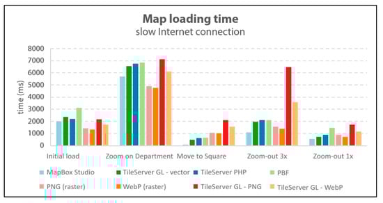
Figure 4.
Results of map loading time (slow Internet connection).
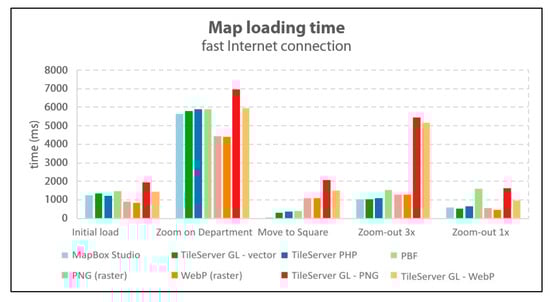
Figure 5.
Results of map loading time (fast Internet connection).
For the first, initial load metric, the applications with pre-generated raster tiles were quicker. The WebP-based application returned slightly better results than the PNG tile application under both slow and fast Internet connections. Raster tiles generated on demand achieved a slower initial loading time of about a second worse than pre-generated equivalents. However, this time was still comparable to the vector tile load time (Figure 4).
Raster tiles generated on demand were the slowest in all of the measured applications on a fast Internet connection (Figure 5). Pre-generated raster tiles were loaded approximately 400 ms quicker than in vector-based solutions. The results showed that raster tiles generated on demand had the worst results in all interactions with the map. A delay of about three seconds was observed in zooming out three zoom-levels. The reason for the quicker retrieval of raster tiles in the “Zoom in on the Department” interaction is that vector tiles also load fonts and labels, which are generated according to a complex algorithm. The result, however, is a map with neat and non-overlapping descriptions. The reason for longer loading time of raster tiles generated on-demand is therefore obvious; generation at the server requires additional time compared to other tiles only downloaded from storage. The client-side (web browser) also requires also more computing for vector tiles, which could be the reason for the longer loading time of vector tiles.
4.4. Download Time for One Tile
Since the map loading time comparison was encumbered by the duration parameter in most interactions, the average downloading times for single tiles were also compared. The total time was the sum of the time for geometry and fonts to load, as these load simultaneously. The resulting time was calculated only from requests when the download was successfully completed. The results are shown in Figure 6 and Figure 7, which show that the vector solution based on TileServer GL (running on the Amazon cloud) was the quickest. The slowest vector tiles were from the solution storing data in a folder structure in PBF format located on the Wedos web host. The average download time of the raster tiles was comparable. Raster tiles generated on demand from vectors were significantly worse in this metric, the difference being up to ten times greater when the user zoomed out more than three levels. A specific issue was observed with the download time metric. Vector tiles consist of two parts: geometry and fonts, which are loaded simultaneously. A visual analysis revealed that the download times for fonts did not differ much from the download time for geometry. Additionally, fonts (from which the label is made) are integral parts of tiles, and without fonts, the data would not be complete.
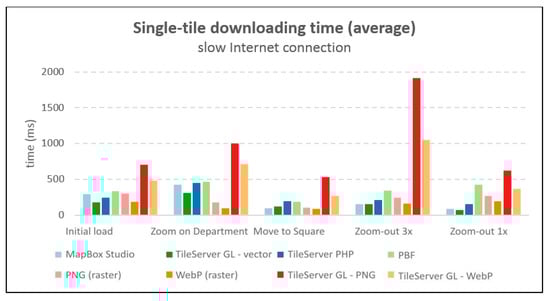
Figure 6.
Results of single-tile downloading times (slow Internet connection).
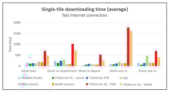
Figure 7.
Results of single-tile downloading times (fast Internet connection).
4.5. Number of Server Requests
As well as each tile’s loading times, the differences in how tiles are downloaded can also be expressed in the number of hits per interaction. The number of these requests corresponds to the number of attempts to download tiles. At initial loading, the number of requests also includes a request to download the Mapbox GL library, style, and site icon. Figure 8 and Figure 9 show the number of all requests in red, and the number of successfully completed requests (i.e., the number of correctly downloaded and displayed tiles) in green. A completely green column means that all of the requests were terminated by data download.
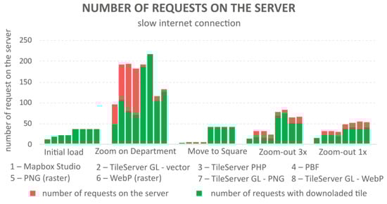
Figure 8.
Results of the number of requests on the server (slow Internet connection).
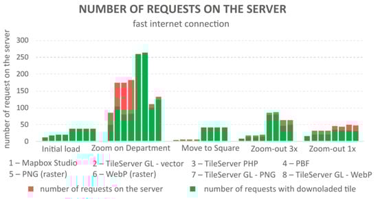
Figure 9.
Results of the number of requests on the server (fast Internet connection).
The values at initial loading and in the “Pan to the Square” interactions were independent of the Internet connection (i.e., the same number of tiles were loaded each time). For the remaining interactions, the values were different. In most cases, fewer requests were sent on a slower connection than (Figure 8) on a faster connection (Figure 9), the reason being that only a fraction of requests from each zoom level could be sent across a range of zoom levels on a slower connection (before the user zoomed to the next level).
The use of two data files resulted in a greater number of failed requests for vectors in “Zoom in on the Department”. When a map was loaded, the application displayed tiles from the OpenMapTiles, airport, and border layers. However, only those tiles that contained data were created, while other tiles were not available. The server response to the request for these tiles was “204 – No Content”, which is the notification of a successful request with no data. Applications with a high number of failed requests are therefore not caused by an error. Mapbox Studio uses only one file, and therefore sends out half the number of requests than other vector tile applications.
The number of requests is a metric that satisfactorily reveals the differences in data retrieval at zoom levels of 15 or higher. While Mapbox Studio downloads only one new tile, and other vector applications download two tiles, raster applications need to download 40 tiles for the same request. In a zoom movement from level 17 to level 14, Mapbox downloaded six tiles, while applications with pre-generated raster tiles sent 76–85 requests and downloaded 68–80 tiles, depending on the connection speed. The server load was therefore many times greater for raster tile solutions, the reason being that vector tile-based applications retrieved the most detailed geometry at level 14 and then displayed the same data (that might otherwise have been styled). For a raster solution, the appropriate tile must be available and downloaded at each level; if not, the image is blurred. The reason for the difference between several requests on the slow and the fast Internet connections is given by the use of a cache. With a faster connection, the client has more time to send additional requests to download the surrounding tiles into the cache.
4.6. Size of Downloaded Data
The final measured metric was the size of the downloaded data for each interaction. The measured values corresponded to the sum of the sizes of all successfully downloaded tiles including fonts for labelling in the case of vector tiles during an interaction.
Figure 10 and Figure 11 show that the amount of data downloaded was comparable in all requests in the vector-based solution. The results showed a corresponding number of successful requests on the server. Raster tiles exhibited large differences. Applications with WebP tiles always downloaded three times less data than the same application with PNG tiles, except during initial loading. Applications with pre-generated tiles captured more data in all interactions than applications with tiles generated on the fly. The reason for a greater amount of downloaded data for vector tiles is because most of the overall size was assigned to labelling, especially during initial loading, when font size accounted for more than half of the downloaded data.
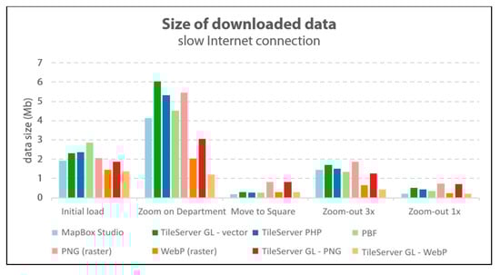
Figure 10.
Results of the size of the downloaded data (slow Internet connection).
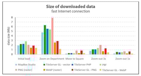
Figure 11.
Results of the size of downloaded data (fast Internet connection).
Raster tiles showed a dependency on the Internet connection with Internet speed reflected in the amount of downloaded data: the faster the Internet, the more tiles can be transmitted and therefore the greater the amount of data downloaded. More data were also downloaded with vector tiles on a fast connection (Figure 11) than a slow connection (Figure 10), and the number of successfully completed requests was comparable to or even greater than on a slow connection. As in the previous test, the reason was the use of a web cache.
4.7. Browsers and Devices
This section provides a comprehensive overview. According to [57], the range of browsers and devices “is one of the great challenges in web development”. Various browsers and devices may be run with limited capabilities [57]. Cross-browser (cross-device) testing is the practice of making sure that web application is supported across several browsers (devices). The authors conducted ad hoc cross-browser and cross-device tests, though generally, user-end load testing is a complex and separate component of overall testing. To incorporate a well-prepared user-load test, a distinct methodology, workflow, tools, and hardware other than that used in this experiment described by this article is required. The authors have therefore decided to continue their research and include new metrics such as user-end loading and browsers/devices/operating systems, and further results will be shared in the future. On the other hand, this chapter discusses a preliminary comparison for the broader analysis of the previous findings.
Several stable browsers were tested on a fast Internet connection: Chrome (78.0.3904.108), Microsoft Edge (42.17134.1098.0), Firefox (69.0.1), and Opera (65.0). The map did not load at all on Safari for Windows. The hardware specification was the same as mentioned in Section 4.1. The experiment recorded the loading time metrics for a comparison between the browsers. The time and size of initial loading for both raster (Tileserver GL - PNG) and vector (Mapbox GL JS) formats were measured ten times using the native development console in each browser. The results in Figure 12 show that the different browsers partially contribute to load metrics. Microsoft Edge transferred significantly less data than the other browsers. Microsoft Edge Console does not capture and measure transmitted data in the same way as other browser consoles, therefore the transfer data metric (Figure 12b) is not comparable. The reason is that the size of all files is not shown and count completely, despite a disable cache is turned on. Apart from Microsoft Edge, the recorded times were almost identical in all of the browsers, with variations only in dozens of milliseconds. Firefox transferred less data than Chrome and Opera, and significantly, almost half as much data for PNG tiles. Chrome and Opera demonstrated the same results due to identical browser engines. Web browser engines also affect visual impression and performance, distribution, and a majority on the market being key contributors. Since Chrome and Opera run on an identical engine, Microsoft Edge will soon switch to the Chromium engine [58] and no longer be supported, and the behavior of major web browsers is trending toward being as identical as possible. Finally, Firefox (Gecko engine) rendered the map tiles similarly to Chrome, but more quickly.
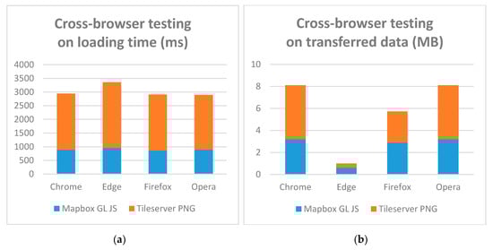
Figure 12.
Results of cross-browser testing: loading time (a); transferred data (b). Note: Capturing of transferred data via Edge is not comparable, see below.
A more significant factor than browsers is the hardware or devices used. The cross-device test was conducted on three devices in the Chrome browser: a personal computer with a commons specification (see Section 4.1), an older Samsung Galaxy Tab 3 tablet (ARM Cortex 1 GHz, 1 GB RAM, Android 4), and a new Redmi 8 smartphone (Octa-core 2 GHz, 4 GB RAM, Android 9). As with the previous testing, the cross-device testing measured loading time metrics for a direct comparison of the three devices. The time and size of the initial loading for raster and vector tiles were measured ten times using remote debugging for Android devices. Figure 13 shows that loading times on the tablet were approximately twice as long than on a smartphone. While the transferred data metric is dependent on display size (a wider display covers a larger area and requires a greater amount of data), no similar dependency exists on loading time, the reason being a combination of hardware and software parameters such as the processor (CPU), memory (RAM), and Android version. The authors assumed that sufficient memory was essential to loading time, however, this assumption could not be supported by any in-depth testing at this point. As above-mentioned, this would require a combination of several tests, which could be a bridge for further research.
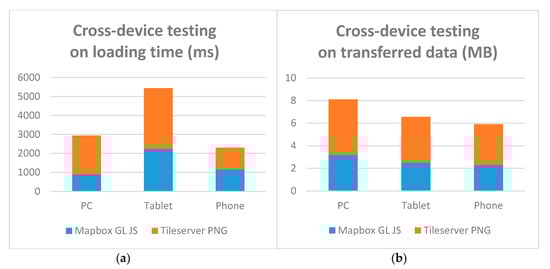
Figure 13.
Results of cross-device testing: loading time (a); transferred data (b).
4.8. Non-Measurable Aspects
Raster and vector solutions differed in some user and technical aspects, but they could not be measured objectively. The user aspect becomes especially significant for website use if map layers are not loaded correctly. From a technical point of view, loading vector and raster tiles is different. While vector tiles load new geometry (and a font set for labelling), raster tiles load a new image. This results in a completely dissimilar experience during map browsing. Typically, quick zoom in/out movements over a map by the user (not the machine, as in the previous sections) may significantly affect user experience and basic cartographical principles [59] (Figure 14). The generalized geometry used in the previous map step is still visible before the geometry for the appropriate zoom level is loaded from vector tiles, although the transition is smooth and continuous. At the same time, descriptions/labels on maps are often missing before they can be fully loaded. However, when raster tiles are loaded, users may observe the phenomenon of previously loaded images remaining on the monitor and are being slowly replaced by new images as they zoom in, as illustrated in Figure 14. At “full point” scale level, (see Section 2.2), a visible blur also momentarily occurs, overlapping the captions from the previously displayed tiles.
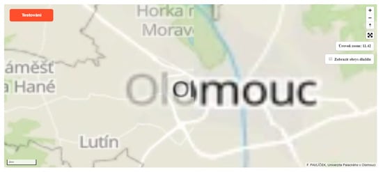
Figure 14.
Visual appearance of raster tiles during fast zoom interaction.
The second negative aspect a user may notice is partially missing labels located at the edge of a tile (Figure 15). This phenomenon only occurs with raster tiles and is a problem associated with tiles generated from the OpenMapTiles project. Vector tiles do not solve this problem since the description is rendered as a separate object above the map data. Furthermore, it is based on a sophisticated algorithm that calculates which labels should be displayed and where to avoid overfilling the map.
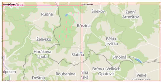
Figure 15.
Incomplete labelling on the edge of the raster tile.
5. Results
Testing was conducted on eight pilot applications to measure the differences in speed and loading between raster and vector tiles using different formats and backend technologies. For this purpose, semi-automatic testing was designed to simulate a user’s handling of a map. In addition to initial loading, the design consisted of four interactions: zooming in on a specific building simulating a point of interest (Department of Geoinformatics building); panning the map to the main square; zooming out three zoom levels; and zooming out one zoom level for comparative purposes. Testing was conducted and recorded in the Google Chrome Console environment, which allows all interactions with the map to be recorded. The data were then exported to a list in HAR format. For each application, ten measurements were recorded on slow (12 MBit/s) and fast (400+ MBit/s) Internet connections at two different times of day. Five measurements were recorded in the morning (7:30–8:30) and five in the afternoon (18:00–19:00). Five attributes were measured in all interactions: total map loading time, number of hits, number of hits successfully completed, average download time per tile, and download size.
The first step was to verify whether the samples collected in the morning and evening differed statistically. To achieve this, an additional 30 measurements were made on the slow Internet connection at both times of day in the application created in Mapbox Studio. Values were obtained for all five interactions, and an F-test of data dispersion was conducted on all interactions to compare the results of the morning and evening measurements. Hypothesis H0 was defined according to the variations of both statistical sets being identical. The results showed that three of the five interactions were statistically different. The other two interactions (“Zoom in on the Department” and “Pan to the Square”) also showed a statistically significant difference. After visual analysis, this difference was discovered to be mainly due to the greater number of extreme values in one of the time periods. Based on these test results, the median of the measured data was therefore selected as the mean value in order to avoid the effect of extreme values on the presented results. The measurements from the morning and evening were also therefore not further differentiated and considered independent for data evaluation purposes.
The testing results were grouped according to the individual metrics examined. Five metrics in total (four measurable and one non-measurable) were performed and evaluated. Table 4 summarizes the general indications of whether raster or vector tiles provided better results in each metric.
Table 4.
Summary of the test results.
The first metric examined was the total map loading time for each interaction. This metric can be partially affected by setting the duration. Duration time was therefore specified (Table 2). Pre-generated raster tiles (except the “Pan to the Square” interaction) showed the best results in this metric. However, applications with raster tiles generated on request were significantly slower. In the case of zooming out three levels, applications with raster tiles were up to five times slower. Fonts and map labels had a large impact in vector-based solutions and extended the total map loading time by up to 2500 ms. If font loading were quicker, vector tile applications would outperform even pre-generated raster tiles.
Due to the above-described effect, the average download speed of one tile was therefore also measured. For vector tiles, the font loading speed for tile labels also had an effect. The average tile download rates in the two categories were comparable to the other categories, except in “Zoom in on the Department” (downloading vector tiles was approximately twice as slow as the pre-generated raster). Raster tiles generated on demand again showed significantly worse results, especially the PNG format. The WebP format was quicker (on a slow connection, up to twice as fast), but still lagged when compared to other applications. For zooming out three levels, the average download time of one tile was up to ten times greater than raster tiles generated on demand.
The third metric examined was the number of requests on the server. This was presented along with the number of requests, resulting in a tile download. The results of this metric showed that vector tile applications downloaded fewer tiles for most interactions than raster tile applications. The most noticeable difference was the “Pan to the Square” interaction, where 1–2 tiles were downloaded for vector, while 40 tiles were downloaded for raster. Due to the long duration of server-side rasterization performed on raster tiles generated on demand, the number of requests for these applications was generally lower than for pre-generated tiles. However, the effect of this on the resulting application speed was negligible. The high number of requests for some vector tile applications that did not end up downloading the tile was due to the amount of data in the second tile file. The boundary and airport layers were not visible on most of the tiles, and the server responded with notifications of successful requests without downloading any data.
The final measured metric was the size of the downloaded data for each interaction. In most cases, the most data required was in applications with pre-generated tiles in PNG format. An application with WebP tiles downloaded about three times less data than PNG. For the “Zoom in on the Department” interaction, the vector tile applications mostly downloaded 4–6 MB of data, while the raster tile applications, except for the pre-generated PNGs, only needed 1–3 MB. For other interactions, the volumes already measured were comparable. The best results from this comparison were almost all the interactions in the WebP tiles, irrespective of pre-generated or on-demand tiles.
In the final testing, the non-measurable aspects of browsing the applications, which included user and technical aspects, were described. The examples recorded while browsing maps demonstrated different loading methods and described problems with raster tiles. These aspects play an aesthetic role in using the map, though may be an important factor for users in selecting which map application to use.
6. Discussion
The authors believe that the testing design and sequence comprehensively covered the major load metrics. It follows the related studies [53] and [54], in which loading time and data size were typically used. The basic metrics included in this article were supplemented by others to cover the most expected metrics from server-end and network testing. Elementary cross-browser and cross-device comparisons were made. Hardware configuration and diverse format/libraries were not involved since the comparisons were primarily not aimed at user-end testing, which is a potential shortcoming of this study. Ad hoc testing showed that the combination of software (browser engines) and hardware (memory) parameters impacted the results significantly. This comparative study has several advantages (+) and disadvantages (−), as follows:
- (+) comparative study as comprehensive performance testing;
- (+) differences between raster and vector tile implementation;
- (+) implementation of the most used metrics;
- (+) technology/format/data storage comparison;
- (+) workflow/metrics/results as recommendations for further studies; and
- (+) testing reflects Internet connections (slow and fast connections; morning and evening).
- (−) only Mapbox Vector Tiles specification (for vector tiles);
- (−) minor metrics not implemented;
- (−) fluctuations in Internet connection not considered; and
- (−) computer performance (different software and hardware configuration) not considered.
The obtained results show that vector tiles may not be suitable for all types of data. The primary challenge is in dataset styles for differing zoom levels. For instance, the default Mapbox Streets style contains about 120 layers that require rendering. Processing and optimizing style during zooming affects the amount of transferred data as well as the time of all the metrics. The difference between raster and vector tiles in generating raster tiles in PNG and WebP formats proved crucial. In certain applications, tiles for the Czech Republic are only stored up to a zoom level of 14. Beyond this level, no more tiles are available, and the last available tile is blurred. The reason is the hardware required to generate raster tiles at higher levels. A total of 55,490 tiles cover the Czech Republic at level 14. At each level, it is four times greater. For example, at level 15, it is 221,960 tiles. In the 15–21 zoom range, there are a total of 1,212,123,560 tiles to cover the Czech Republic only. Tiles were therefore only generated and tested up to level 14, as with the vector tiles.
An in-depth analysis of the results could reveal the causes for the difference between the methods in this study. Some recommendations for web application design were given according to the findings. One of the tested metrics was loading time. Obviously, for both technologies (raster, vector) the loading time of pre-generated tiles was significantly less than the loading time of tiles generated on-demand (generation on the server takes additional time compared to tiles only downloaded from storage). The main reason for using tiles generated on-demand is saving disk space. It appears to be ideal to use a combination of both methods. For low zoom levels and highly frequented areas, it is better to use pre-generated tiles. Detailed zoom levels and peripheral regions (oceans, forests), however, can use pre-generated tiles satisfactorily.
Another metric examined was the size of the downloaded data. If a user frequently changes the zoom level, vector tiles have the advantage of not needing to be re-downloaded and the client browser is able to change their resolution. On the other hand, if a user browses the map at the same zoom level, less data are downloaded with raster tile maps. According to the amount of downloaded data metrics, the better method is vector tile maps. For specialized maps with only a few zoom levels, using raster tiles appears to be better.
The speed of the Internet connection has a significant effect on convenience in working with maps. Faster Internet connections allow maps to be loaded more quickly, but another factor is also affected by Internet connection speed. With faster Internet connection speeds, more requests can be sent by the server, allowing tiles from a larger surrounding area of the currently displayed area to be downloaded. As a result, maps are much smoother to browse due to the use of a cache populated with more downloaded tiles.
The original objective was to use the Leaflet library, which is one of the most popular web mapping libraries. However, it became apparent that the possibilities of working with vector tiles via the Leaflet library are too much limited. Still, at least two other libraries support vector data by default: OpenLayers and ArcGIS API. There is little doubt that vector tile support will soon improve, and other map libraries initially designed to operate with raster tiles can only be expected to implement vector tile support in the future.
More effects on the measured values than simply the applied technology and Internet connection speed can be assumed. Typically, moving applications to an HTTPS server instead of HTTP could have a beneficial effect on download time.
7. Conclusions
The rapid development of web applications has also changed how background maps are rendered. Raster tiles can currently be considered as a regular solution, while the use of vector tiles is becoming more widespread. The main objective of this work was to conduct a study on load metrics by comparing different methods for raster and vector tiles. Testing showed that vector tiles did not always load more quickly than raster tiles. However, their main advantages are in reducing server load and the amount of downloaded data and providing a more user-friendly experience for browsing map applications. Since libraries place labels over maps dynamically, labels as a result do not overlap and maps do not become denser, which is more efficiently adapted for mobile devices. The results of our load testing indicated that the process of generating raster tiles on demand is several times slower than displaying pre-generated tiles. For applications to achieve at least a similar performance to vector tile applications, tiles in the display area must be generated before the user request. These tests showed that in most cases, vector tiles had a better loading time. Raster tiles may be more suitable for applications where access is assumed from sites with a slow Internet connection. As raster tiles are the de facto standard for basemaps today, vector tiles, being similarly popular in the very near future can be expected.
Author Contributions
Rostislav Netek was responsible for the concept, methodology, and analysis. Jan Masopust wrote the article. Frantisek Pavlicek conducted pilot studies and tests. Vilem Pechanec was responsible for overall leading and mentoring. All authors have read and agreed to the published version of the manuscript.
Funding
This research received no external funding.
Acknowledgments
This paper was created within the project "Innovation and application of geoinformatic methods for solving spatial challenges in the real world." (IGA_PrF_2020_027) with the support of Internal Grant Agency of Palacky University Olomouc.
Conflicts of Interest
The authors declare no conflict of interest.
References
- Sample, J.T.; Ioup, E. Tile-Based Geospatial Information Systems. Principles and Practices; Springer: Berlin/Heidelberg, Germany, 2010. [Google Scholar]
- Stefanakis, E. Map Tiles and Cached Map Services. GoGeomatics. Magazine of GoGeomatics Canada. 2015. Available online: http://www2.unb.ca/~estef/papers/go_geomatics_stefanakis_december_2015.pdf (accessed on 5 March 2019).
- Leaflet/Providers Preview. Available online: http://leaflet-extras.github.io/leaflet-providers/preview/ (accessed on 13 December 2019).
- Goodchild, M.F. Tiling Large Geographical Databases; Springer: Berlin/Heidelberg, Germany, 1990; pp. 135–146. ISBN 9783540469247. [Google Scholar]
- Peterson, M.P. Maps and the Internet; Elsevier: London, UK, 2003; ISBN 978-0-08-044201-3. [Google Scholar]
- Jiang, H.; Van Genderen, J.; Mazzetti, P.; Koo, H.; Chen, M. Current status and future directions of geoportals. Int. J. Digit. Earth 2019. [Google Scholar] [CrossRef]
- Veenendaal, B.; Brovelli, M.A.; Li, S. Review of Web Mapping: Eras, Trends and Directions. ISPRS Int. J. Geo-Inf. 2017, 6, 317. [Google Scholar] [CrossRef]
- Zalipynis, R.A.R.; Pozdeev, E.; Bryukhov, A. Array DBMS and Satellite Imagery: Towards Big Raster Data in the Cloud. In Proceedings of the International Conference on Analysis of Images, Social Networks and Texts, Moscow, Russia, 5–7 July 2018; Springer: Cham, Germany, 2018; Voulme 10716, pp. 267–279. [Google Scholar]
- Villar-Cano, M.; Jiménez-Martínez, M.J.; Marqués-Mateu, Á. A Practical Procedure to Integrate the First 1:500 Urban Map of Valencia into a Tile-Based Geospatial Information System. ISPRS Int. J. Geo-Inf. 2019, 8, 378. [Google Scholar] [CrossRef]
- Yao, X.C.; Li, G.H. Big spatial vector data management: A review. Big Earth Data 2018, 2, 108–129. [Google Scholar] [CrossRef]
- Wan, L.; Huang, Z.; Peng, X. An Effective NoSQL-Based Vector Map Tile Management Approach. ISPRS Int. J. Geo-Inf. 2016, 5, 215. [Google Scholar] [CrossRef]
- Zouhar, F.; Senner, I. Web-Based Visualization of Big Geospatial Vector Data. In Proceedings of the The Annual International Conference on Geographic Information Science, Limassol, Cyprus, 17–20 June 2019; Kyriakidis, P., Hadjimitsis, D., Skarlatos, D., Mansourian, A., Eds.; Springer: Cham, Germany, 2020. [Google Scholar] [CrossRef]
- Li, L.; Hu, W.; Zhu, H.; Li, Y.; Zhang, H. Tiled vector data model for the geographical features of symbolized maps. PLoS ONE 2017, 12, e0176387. [Google Scholar] [CrossRef] [PubMed]
- Yang, C.; Goodchild, M.F.; Huang, Q.; Nebert, D.; Raskin, R.; Xue, Y.; Bambacus, M.; Faye, D. Spatial cloud computing: How can the geospatial sciences use and help shape cloud computing? Int. J. Digit. Earth 2011, 4, 305–329. [Google Scholar] [CrossRef]
- Stefanakis, E. Web mercator and raster tile maps: Two cornerstones of online map service providers. Geomatica 2017, 71, 100–109. Available online: http://www.nrcresearchpress.com/doi/10.5623/cig2017-203 (accessed on 5 March 2019). [CrossRef]
- MapTiler. Tiles á la Google Maps: Coordinates, Tile Bounds and Projection. 2018. Available online: https://www.maptiler.com/google-maps-coordinates-tile-bounds-projection/ (accessed on 5 March 2019).
- OpenGIS Web Map Tile Service Implementation Standard. Available online: https://www.opengeospatial.org/standards/wmts (accessed on 5 March 2019).
- Zavadil, F. Software pro zobrazování mapových dlaždic. Ph.D. Thesis, České vysoké učení technické, Praha, Czech Republic, 2013. [Google Scholar]
- Peterson, M.P. The Tile-Based Mapping Transition in Cartography; Springer: Berlin/Heidelberg, Germany, 2012; pp. 151–163. Available online: http://link.springer.com/10.1007/978-3-642-19522-8_13 (accessed on 5 March 2019).
- Fu, P.; Sun, J. Web GIS: Principles and Applications; ESRI Press: Redlands, CA, USA, 2011; ISBN 978-1-58948-245-6. [Google Scholar]
- Noskov, A. Computer Vision Approaches for Big Geo-Spatial Data: Quality Assessment of Raster Tiled Web Maps for Smart City Solutions. In 7th International Conference on Cartography and GIS; Bulgarian Cartographic Association: Sofia, Bulgaria, 2018; pp. 296–305. [Google Scholar] [CrossRef]
- Antoniou, V.; Morley, J.; Haklay, M.M. Tiled Vectors: A Method for Vector Transmission over the Web. In Proceedings of the International Symposium on Web and Wireless Geographical Information Systems, Maynooth, Ireland, 7–8 December 2009; Springer: Berlin/Heidelberg, Germany, 2009; pp. 56–57. Available online: http://link.springer.com/10.1007/978-3-642-10601-9_5 (accessed on 5 March 2019).
- Gaffuri, J. Toward Web Mapping with Vector Data. In Proceedings of the The Annual International Conference on Geographic Information Science, Columbus, OH, USA, 18–21 September 2012; Springer: Berlin/Heidelberg, Germany, 2012; pp. 87–101. Available online: http://link.springer.com/10.1007/978-3-642-33024-7_7 (accessed on 5 March 2019).
- Shang, X. A Study on Efficient Vector Mapping with Vector Tiles based on Cloud Server Architecture. Ph.D. Thesis, University of Calgary, Calgary, AB, Canada, 2015. [Google Scholar]
- Netek, R.; Brus, J.; Tomecka, O. Performance Testing on Marker Clustering and Heatmap Visualization Techniques: A Comparative Study on JavaScript Mapping Libraries. ISPRS Int. J. Geo-Inf. 2019, 8, 348. [Google Scholar] [CrossRef]
- Netek, R.; Dostalova, Y.; Pechanec, V. Mobile Map Application for Pasportisation of Sugar Beet Fields. Listy Cukrovarnické. a Řepařské 2015, 131, 137–140. [Google Scholar]
- Bertolotto, M.; Egenhofer, M.J. Progressive Transmission of Vector Map Data over the World Wide Web. GeoInformatica 2001, 5, 345–373, ISSN 1573-7624. [Google Scholar] [CrossRef]
- Mapbox Documentation. Available online: https://docs.mapbox.com/ (accessed on 5 March 2019).
- Korotkiy, M. Implementations of Mapbox MBTiles spec. 2018. Available online: https://github.com/mapbox/mbtiles-spec/wiki/Implementations (accessed on 5 March 2019).
- OPENMAPTILES. Open Vector Tile Schema for OpenStreetMap Layers. 2019. Available online: https://openmaptiles.org/schema/ (accessed on 5 March 2019).
- Mapbox Studio. Available online: https://www.mapbox.com/mapbox-studio/ (accessed on 13 December 2019).
- JSON Schema–Specification. Available online: https://json-schema.org/specification.html (accessed on 13 December 2019).
- Mapbox, G.L. JS-API Reference. Available online: https://docs.mapbox.com/mapbox-gl-js/api/ (accessed on 13 December 2019).
- Tileserver, G.L. Available online: http://tileserver.org/ (accessed on 13 December 2019).
- Maputnik Editor. Available online: https://maputnik.github.io/editor/ (accessed on 13 December 2019).
- Amazon Web Services: Amazon EC2. Available online: https://aws.amazon.com/ec2/ (accessed on 13 December 2019).
- Github: Tileserver PHP. Available online: https://github.com/maptiler/tileserver-php (accessed on 13 December 2019).
- Github: Tippecanoe. Available online: https://github.com/mapbox/tippecanoe (accessed on 13 December 2019).
- MDN. Cross-Origin Resource Sharing (CORS)–HTTP. 2019. Available online: https://developer.mozilla.org/en-US/docs/Web/HTTP/CORS (accessed on 5 March 2019).
- Netek, R. Interconnection of Rich Internet Application and Cloud Computing for Web Map Solutions. In Proceedings of the 13th SGEM GeoConference on Informatics, Geoinformatics and Remote Sensing, Albena, Bulgaria, 16–22 June 2013; Volume 1, pp. 753–760, ISBN 978-954-91818-9-0; ISSN 1314-2704. [Google Scholar]
- García, R.; de Castro, J.P.; Verdú, E.; Verdú, M.J.; Regueras, L.M. Web Map Tile Services for Spatial Data Infrastructures: Management and Optimization. In Cartography-A Tool for Spatial Analysis; IntechOpen: London, UK, 2012. [Google Scholar] [CrossRef]
- Fábry, J.; Feciskanin, R. Publikovanie geodát vo forme vektorových dlaždíc a porovnanie výkonu s rastrovými dlaždicami. Geografický Časopis, Bratislava, Slovakia 2019, 71, 283–293. [Google Scholar] [CrossRef]
- Fujimura, H.; Sanchez, O.M.; Ferreiro, D.G.; Kayama, Y.; Hayashi, H.; Iwasaki, N.; Mugambi, F.; Obukhov, T.; Motojima, Y.; Sato, T. Design and Development of the un Vector Tile Toolkit. Int. Arch. Photogramm. Remote Sens. Spatial Inf. Sci. 2019, XLII-4/W14, 57–62. [Google Scholar] [CrossRef]
- Kefaloukos, P.K.; Vaz Salles, M.; Zachariasen, M. TileHeat: A framework for tile selection. In Proceedings of the ACM International Symposium on Advances in Geographic Information Systems, Beach, CA, USA, 6–9 November 2012; pp. 349–358. [Google Scholar]
- Ingensand, J.; Nappez, M.; Moullet, C.; Gasser, L.; Ertz, O.; Composto, S. Implementation of Tiled Vector Services: A Case Study. Available online: https://pdfs.semanticscholar.org/d6ed/d2656c0efbcc12d357fee0571398c7415f45.pdf (accessed on 30 December 2019).
- Braga, V.G.; Corr, S.L.; Rodrigues, V.J.d.S.; Cardoso, K.V. Characterizing User Behavior on Web Mapping Systems Using Real-World Data. In Proceedings of the IEEE Symposium on Computers and Communications (ISCC), Natal, Brazil, 25–28 June 2018; pp. 1056–1061. [Google Scholar] [CrossRef]
- Pridal, P. Tile Based Map Publishing with WMTS TileServer, MapTiler and TileMill. FOSSGIS 2013. Available online: https://fossgis-konferenz.de/2013/programm/events/604.en.html (accessed on 30 December 2019).
- What are Vector Tiles and Why You Should Care. Available online: https://www.maptiler.com/blog/2019/02/what-are-vector-tiles-and-why-you-should-care.html (accessed on 30 December 2019).
- Improve the Performance of Mapbox GL JS Maps. Available online: https://docs.mapbox.com/help/troubleshooting/mapbox-gl-js-performance/ (accessed on 30 December 2019).
- Github: Improve’ Perceived Performance’ by Preloading Lower Zoom Level Tile. Available online: https://github.com/mapbox/mapbox-gl-js/issues/2826 (accessed on 30 December 2019).
- Github: Performance Testing. Available online: https://github.com/maptiler/tileserver-gl/issues/9 (accessed on 30 December 2019).
- Github: Slow Carto Tile Performance. Available online: https://github.com/openstreetmap/operations/issues/268 (accessed on 30 December 2019).
- Cadell, W. Map Tile Performance. Maptik. 2015. Available online: https://maptiks.com/blog/map-tile-performance/ (accessed on 30 December 2019).
- GIScloud: Realtime Map Tile Rendering Benchmark: Vector Tiles Vs. Raster Tiles. Available online: https://www.giscloud.com/blog/realtime-map-tile-rendering-benchmark-rasters-vs-vectors/ (accessed on 30 December 2019).
- Adamec, L. Vector tiles in web cartography. Ph.D. Thesis, Masaryk University, Brno, Czech Republic, 2016. [Google Scholar]
- Schön, O. Česko si Pohoršilo v Rychlosti Připojení k Internetu, Mobilní sítě jsou ale Nadprůměrné. 2017. Available online: https://tech.ihned.cz/internet/c1-65993950-cesko-si-pohorsilo-v-rychlosti-pripojeni-k-internetu-mobilni-site-jsou-ale-nadprumerne (accessed on 5 March 2019).
- MDN: Introduction to Cross Browser Testing. Available online: https://developer.mozilla.org/en-US/docs/Learn/Tools_and_testing/Cross_browser_testing/Introduction (accessed on 30 December 2019).
- ZDNet: Microsoft’s Chromium-based Edge Browser to be Generally Available 15 January 2020. Available online: https://www.zdnet.com/article/microsofts-chromium-based-edge-browser-to-be-generally-available-january-15-2020/ (accessed on 30 December 2019).
- Brychtova, A.; Popelka, S.; Dobesova, Z. Eye-tracking methods for investigation of cartographic principles. In Proceedings of the 12th International Multidisciplinary Scientific Geoconference, Albena, Bulgaria, 17–23 June 2012; Volume 4, pp. 1041–1048. [Google Scholar]
© 2020 by the authors. Licensee MDPI, Basel, Switzerland. This article is an open access article distributed under the terms and conditions of the Creative Commons Attribution (CC BY) license (http://creativecommons.org/licenses/by/4.0/).