A Novel Indoor Structure Extraction Based on Dense Point Cloud

Abstract

Herein, we propose a novel indoor structure extraction (ISE) method that can reconstruct an indoor planar structure with a feature structure map (FSM) and enable indoor robot navigation using a navigation structure map (NSM). To construct the FSM, we first propose a two-staged region growing algorithm to segment the planar feature and to obtain the original planar point cloud. Subsequently, we simplify the planar feature using quadtree segmentation based on cluster fusion. Finally, we perform simple triangulation in the interior and vertex-assignment triangulation in the boundary to accomplish feature reconstruction for the planar structure. The FSM is organized in the form of a mesh model. To construct the NSM, we first propose a novel ground extraction method based on indoor structure analysis under the Manhattan world assumption. It can accurately capture the ground plane in an indoor scene. Subsequently, we establish a passable area map (PAM) within different heights. Finally, a novel-form NSM is established using the original planar point cloud and the PAM. Experiments are performed using three public datasets and one self-collected dataset. The proposed plane segmentation approach is evaluated on two simulation datasets and achieves a recall of approximately 99%, which is 5% higher than that of the traditional plane segmentation method. Furthermore, the triangulation performance of our method compared with the traditional greedy projection triangulation show that our method performs better in terms of feature representation. The experimental results reveal that our ISE method is robust and effective for extracting indoor structures.

1. Introduction

Recently, the generation of three-dimensional (3D) models of the environment has garnered significant interest in various fields, e.g., building renovation [1], indoor navigation [2], architecture [3], and facility management [4,5]. With the availability of mature technology for data collection, rich environment information can be captured through many platforms such as light detection and ranging [6], RGB-D cameras [7], and stereo cameras [8]. Subsequently, efficient and robust structure extractions based on acquired data became a popular research topic. The purpose of indoor structure extraction (ISE) is to capture the salient structure and to provide a robust description of the interior layout. Traditional manual ISE is tedious and requires excessive manual intervention. Compared with the structure extraction of the outdoor environment [9,10], ISE is more challenging in terms of three aspects: it requires (a) a higher quantity of clutter, (b) a more complex geometry, and (c) a more uneven-distributed occlusions.

According to the data type, ISE methods are generally classified into two major categories: (1) ISE based on image data using formatted images and small data memory, subject to illumination changes, for which some studies based on image data have been performed [11,12,13], and (2) ISE based on point cloud data using an unstructured point cloud, favorable spatial topology, and a large memory footprint, for which studies have also been performed [14,15,16,17]. Furthermore, methods combining image and point clouds have been proposed [18,19,20], and video has been exploited [21,22,23].

Moreover, the resulting form of ISE can be classified into three types: feature structure map (FSM), semantic structure map (SSM), and navigation structure map (NSM). An FSM is constructed based on one or more types of indoor structures. Robust indoor structures can be represented accurately; however, topological associations of features are not considered. An SSM is generated using a semantic feature from an indoor scene. The major indoor layout or structure primitives can be reconstructed; however, a detailed description of some structures is insufficient and some semantic features are inessential for location and navigation. The NSM is mainly used to emphasize obstacle target detection, topological relations, and passable areas in indoor spaces; however, the indoor structure is not organized in a unified and reasonable form.

Herein, we propose a novel ISE method based on a point cloud. The result of our ISE comprises an FSM and an NSM. To construct the FSM, a novel two-stage region growing plane segmentation algorithm was used to extract planar features (the original planar point cloud) with better integrity. Subsequently, planar inliers were simplified using a quadtree-based segmentation algorithm. Finally, two triangulation strategies in the boundary and interior were used to reconstruct the planar structure. To construct the NSM, we used a novel NSM comprising a passable area map (PAM) within different heights and the original planar point cloud. Moreover, our NSM was constructed based on the Manhattan world assumption, which pertains to the statics of the city and indoor scenes. It states that an indoor scene is built on a Cartesian grid where surpatches in the world are aligned with one of three dominant directions. Our main contributions are four-fold: (1) The proposed two-stage region growing plane segmentation algorithm improves the integrity of the plane and the robustness of the FSM. (2) The quadtree simplification method can significantly reduce data memory, and the proposed triangulation strategy can emphasize the connection between the boundary and interior structure. (3) For NSM construction, our method can capture the ground well from indoor point clouds without additional prior constraints. (4) The proposed novel NSM form not only can indicate a passable area for path planning but also can serve as a reference feature map to improve the efficiency and robustness of indoor robot navigation.

The remainder of the paper is organized as follows. Related studies are reviewed in Section 2. Our ISE method is introduced in detail in Section 3. The experimental details are presented in Section 4. The experimental results are discussed and analyzed in Section 5. The conclusions are provided in Section 6.

2. Related Studies

To date, a few studies regarding ISE based on indoor point cloud data have been performed.

• (A) FSM

An FSM is used to identify and model the dominant visible structural components of an indoor environment. Some researchers have optimized the reconstruction of certain structure types and decimated redundant information. Other researchers automatically recovered the architectural components in some extreme conditions, such as those involving occlusion and many clusters. Some researchers used the triangulation method based on extracted features to reconstruct the indoor structure. Ma et al. [24] presented a method for the efficient triangulation and texturing of planar surfaces in a large point cloud. Point- and polygon-based triangulation methods are used to yield an accurate and robust planar triangulation. This technology involves random sample consensus (RANSAC)-based plane segmentation. The detected plane structure is decimated using a quadtree-based method. Each decimated plane segment is partitioned into the boundary and interior, point-based triangulation is performed between the ordered boundary and interior points, and polygon-based triangulation is performed directly on the inner vertices. Finally, textures of plane segments are generated by projecting the vertex colors of the dense planar segment onto a two-dimensional (2D) RGB texture. Feichter and Hlavacs [25] extracted planar features using RANSAC. Subsequently, the boundary of the plane was detected using the alpha shape boundary algorithm and the plane was triangulated with constrained Delaunay triangulation. Furthermore, some researchers used the Hough transform to detect indoor robust structures and to reconstruct indoor FSMs based on extracted structures, such as wall surfaces [26,27]. Other methods have been proposed for indoor FSM reconstruction, such as a novel coarse-to-fine planar shape segmentation method [28], graph-cut optimization [29], employment of regularities existing on facades [30], a flatness-based algorithm [31], and carving [32]. Recently, some unsupervised segmentation methods for feature extraction have been presented, such as region growing based on geometrical continuities [33], voxel-based semantic segmentation [34], over-segmentation using spatial connectivity and geometric features [35], and region growing based on Octree [36].

• (B) SSM

Armeni et al. [37] utilized geometric priors acquired from parsing and reincorporating detected elements to update the spaces discovered. Ochmann et al. [38] constructed a probabilistic model to estimate the updated soft assignments of points to room labels. Kwadjo et al. [39] proposed a novel 2D matrix template representation of walls that eased operations, such as the room layout and opening detection in polynomial time. Yang et al. [40] defined three types of structural constraints (semantic, geometric, and topological constraints) of architectural components in scene representation. Shi et al. [41] used a minimum graph cut algorithm in room clusters to detect wall-surface objects. Wang et al. [42] proposed a novel semantic line framework-based modeling building method to optimize line structures detected using the proposed conditional generative adversarial nets. Xiong and Huber [43] used a conditional random field model to discover contextual information to aid the construction of a 3D semantic model. Some machine learning methods have been proposed for learning unique features of different structure types and labeling structures [44,45].

• (C) NSM

Researchers have proposed the construction of navigation graphs based on certain semantic-based models [46,47]. Some flexible space subdivision (FSS) frameworks have been presented to account for advanced constraints during navigation or for identifying the spaces for indoor navigation [48,49]. Zlatanova et al. [50] presented a framework that specifically emphasized physical and conceptual subdivisions of indoor spaces for supporting indoor localization. Taneja et al. [51] presented algorithms for the automated generation of three different types of navigation models, i.e., centerline-based network, metric-based, and grid-based navigation models, for map-matching of indoor positioning data. Flikweert et al. [52] constructed an indoor navigation graph based on the IndoorGML structure, where nodes were placed in spaces, doors, slopes, and stairs and the connectivity relationships among them was determined from a node-relation graph. Boguslawski et al. [53] proposed a novel automated construction of the variable density network to determine egress paths in dangerous environments. Li et al. [54] designed a deep network combining PointNet with the Markov random field to identify single objects from the point cloud more precisely for indoor navigation. Nakagawa and Nozaki [55] proposed a method that included object classification, navigable area estimation, and navigable path estimation to construct a geometrical network model for indoor navigation. Liu et al. [56] designed an indoor spatial navigation model to support navigation and logical models from floor plans. Abdullah et al. [57] proposed an enhanced IndoorGML conceptual model (Unified Modelling Language (UML) class diagram) to avoid misunderstanding; the conceptual model can map the classes of the standard more effectively. Based on Milner’s bigraphical models, Walton et al. [58] designed bigraphs to provide formal algebraic specifications that independently represented the agent as well as the place locality (e.g., building hierarchies) and connectivity (e.g., path-based navigation graphs).

However, some issues are present in ISE based on point clouds: (1) some ISE methods using machine learning require a large amount of diverse learning sample data, and currently, the labeling data of the point cloud are less than that of the image. The performance of the method is subject to tedious model training, which may compromise the efficiency of ISE. (2) Some ISE methods are performed under significant manual intervention, and they are affected by irrational parameter settings. Excessive manual operations and irregular parameter settings will significantly impair the applicability of the algorithm; (3) although ISE can extract the structure with high accuracy, the integrity of the structure is not guaranteed. The complete structure is essential and beneficial to ISE.

Our ISE method does not require a labeled point cloud, and the result is a hybrid extraction including an FSM and an NSM. The method can complete model representation of an indoor prominent planar structure robustly and can indicate an indoor passable area. Furthermore, it can effectively manage the salient planar structure for indoor localization. Owing to the superiority of the hybrid result form, our ISE result can be applied to more fields. Through the effective management of parameters, massive manual labor is not required for FSM construction. For NSM construction, our method can capture the ground plane robustly without other additional constraints.

3. Method

A flowchart of the proposed ISE method is shown in Figure 1. The input is a raw dense non-structured point cloud, and the output comprises an FSM and an NSM. The processing pipeline comprises four stages:

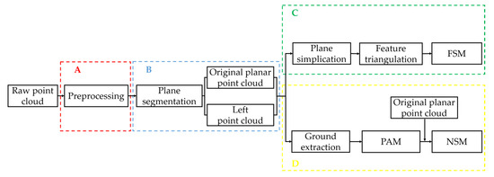
Figure 1. The overall processing pipeline of the proposed method.

• Preprocessing: the raw point cloud data are processed to eliminate invalid and noise points. Subsequently, the data volume is reduced significantly via downsampling.
• Plane segmentation: The planar structure is captured through a hybrid two-staged region-growing algorithm. Subsequently, the preprocessing point cloud is classified into the original plane and left point clouds.
• FSM construction: After plane segmentation, each planar point cloud is classified into inliers and boundaries. Subsequently, different triangulation strategies are adopted in the two parts. Finally, an FSM (e.g., a planar mesh model) based on a planar structure is generated.
• NSM construction: A novel ground plane is proposed based on indoor structure analysis under the Manhattan world assumption. Subsequently, an obstacle map within different heights and initial passable areas are constructed. Finally, a novel NSM comprising an original planar point cloud and a PAM is generated.

3.1. Preprocessing

The preprocessing comprises three steps: invalid point removal, statistical filtering, and voxel filtering. First, the invalid data type, “NAN”, is removed in the raw point cloud and $Ma{p}^I$ is obtained. Subsequently, some error and noise points generated during scanning or stitching are eliminated via statistical filtering using Equation (1), and $Ma{p}^S$ is acquired. Finally, voxel filtering with voxel size ($r\ast r\ast r$), a downsampling method, is performed to leverage the data memory. In addition, the sampling point cloud data $Ma{p}^V$ is preserved.

$$\{pt\to noise | pt \in Ma{p}^I, nad\left(pt\right)>\epsilon \ast \overline{d} \},$$

(1)

where $nad\left(pt\right)$ is the distance average between $pt$ and $n_k$ neighbor points in $Ma{p}^I$, $\epsilon$ is a scale coefficient ($\epsilon =3$), and $\overline{d}$ is the average distance of all points and their neighbor points in $Ma{p}^I$.

3.2. Two-Staged Region Growing Plane Segmentation

In indoor scenes, piecewise planar structures overwhelm other surface structures. Therefore, we reconstructed the indoor structure based on a planar feature. Two prominent approaches exist for plane segmentation: model fitting and region growing. The model fitting method is implemented on a predefined mathematical model. Two widely used models are random sample consensus (RANSAC) [59] and the Hough transform [60]. In the model fitting method, the spatial topology cannot be considered in a 3D space; hence, discontinuities may occur in the planar feature. The existing region growing method is sensitive to the computation accuracy of the growing conditions, which may impair the integrity of the planar feature. Therefore, we proposed a hybrid two-staged region growing plane segmentation to manage the boundary structure details more effectively. Our method comprises point-based region growing (stage 1) and plane-based region growing (stage 2).

3.2.1. Point-Based Region Growing

In Algorithm 1, the point-based region growing is illustrated. The algorithm uses $Ma{p}^V$ as input and generates a preliminarily segmented plane $P{l}^A$. The growing conditions, including the normal angle requirement and point-to-plane distance constraint, are adopted. In the growing analysis, the neighbor points with qualified normal are preserved in candidate seeds. In Equation (2), the point-to-plane distance is further calculated for points with unqualified normal. Points with a point-to-plane distance less than the distance threshold ${\delta }_1$ will be preserved in the growing planar segment but not for the candidate seeds. The point cloud $Ma{p}^V$ is partitioned into the preliminary plane $P{l}^A$ and the remaining points $Rp$ after the point-based region grows.

$$d_{ptp}=\frac{\left|⟨p_s,n_t⟩ + d_t\right|}{\sqrt{{\left(n_t\right)}_x^2+{\left(n_t\right)}_y^2+ {\left(n_t\right)}_z^2}},$$

(2)

where $p_s$ is the query point, ($n_t$,$d_t$) is the parameter of the plane equation, and $n_t$ is the normal to the plane.

Algorithm 1 Point-based region growing (Stage 1)

1: Input: Point cloud $Ma{p}^V \left\{p{t}_i\right| p{t}_i \in Ma{p}^V\}$, neighbor finding function $\mathsf{\Omega }(.)$, angle threshold

2: ${\theta }_1$ distance threshold ${\delta }_1$.

3: Output: Preliminary segmented plane point cloud {$P{l}^A$}

4: Initialize: $\mathrm{Plane}\mathrm{point}\mathrm{cloud}\mathrm{label}i{d}_{plane}\leftarrow 0$,$\mathrm{point}\mathrm{neighbors}\left\{Nb{d}_i\right\} \leftarrow \{\varnothing \}$, point normals

5: $\left\{Nm{l}_i\right\}\leftarrow$ $\{\varnothing \}$, point curvature {${\mathrm{Cv}}_i$}$\leftarrow \{\varnothing \}$, region label $\left\{Rl\right\}$ $\leftarrow$ {$R{l}_i$| $R{l}_i= -1, i= 0,1\dots$

6: $\mathrm{size}\left(Map\right)$}, {$Nb{d}_i$}$\leftarrow \mathsf{\Omega }\left(p{t}_i\right)$,$\left\{Nm{l}_i\right\}\leftarrow$ PCA ($Nb{d}_i$),${\mathrm{Cv}}_i\leftarrow$ EVD ($Nb{d}_i$), point order

7: $\left\{\mathrm{Po}\right\}\leftarrow$ sort points according to curvature in ascending order.

8: Candidate seeds $\left\{S_c^A\right\}\leftarrow \{\varnothing \}$, insert the minimum curvature point in $\left\{Po\right\}$ to $\left\{S_c^A\right\}$

9: if there is still $R{l}_i$ equals to −1

10: while $\left\{S_c^A\right\}$ is not empty do

11:   current seed $Cs\leftarrow$ the first element in $\left\{S_c^A\right\}$, remove $Cs$ from $\left\{S_c^A\right\}$

12:   for $\mathrm{idx} \in \left\{Nb{d}_i\right\}\mathrm{of}Cs$

13:    angle $\leftarrow$ compute angle between $\left\{Nm{l}_i\right\} \mathrm{of} idx \mathrm{and}\left\{Nm{l}_i\right\} \mathrm{of} Cs$

14:    if angle < ${\theta }_1$

15:     insert $\mathrm{idx}$ to $\left\{S_c^A\right\}, R{l}_{idx}\leftarrow i{d}_{plane}$

16:    end if

17:    else

18:     dist $\leftarrow$ compute distance between $p{t}_{idx}$ and the fitting local plane of $Cs$

19:     if $\mathrm{dist}<{\mathsf{\delta }}_1$

20:      $R{l}_{idx}\leftarrow i{d}_{plane}$

21:     end if

22:     else

23:      $R{l}_{idx}\leftarrow$−2

24:     end else

25:    end else

26:   end for

27:  end while

28:  $i{d}_{plane}$ increases by 1

29: end if

30: if $R{l}_i$ > −1

31:  Assemble $p{t}_i$ to $P{l}_i^A$ according to $R{l}_i$

32: end if

Where PCA is principal component analysis, and EVD is eigenvalue decomposition.

3.2.2. Plane-Based Region Growing

After the point-based region growing, some plane points, $Rp$, such as the boundary points, remained unclassified owing to the limitation of the growing condition. Plane-based region growing was adopted to further process unclassified plane points.

(1)

Remaining point updates

As shown in Equation (3), we adopted a point quantity threshold ${\zeta }_1$ to filter small planes $P{l}^{ti}$ and to scatter them back into $Rp$. Subsequently, the updated remaining point cloud $R{p}^u$ is obtained.

$$R{p}^u=Rp+ P{l}^{ti}, P{l}^{ti}= \left\{P{l}_i^A\right|n\left(P{l}_i^A\right)< {\zeta }_1\},$$

(3)

where $n\left(P{l}_i^A\right)$ denotes the point quantity of plane point cloud $P{l}_i^A$.

(2)

Plane Growing

Neighbor points $N{p}_i^B$ for all points of $P{l}_i^A$ are established in $R{p}^u$, and repetitive points in $N{p}_i^B$ are removed. A growing process similar to stage 1 was performed on $N{\mathrm{p}}_i^B$ and $R{p}^u$. However, only the distance growing condition was considered. In Equation (4), each plane point cloud $P{l}_i^B$ comprises qualified unclassified points $P{t}^{qua}$ and the corresponding preliminary plane $P{l}_i^A$ after the plane-based region grows.

$$P{l}_i^B=P{l}_i^A+ P{t}^{qua},P{t}^{qua}= \{pt |d\left(pt, P{l}_i^A\right)< {\delta }_2, pt \in N{p}_i^B\},i=0,1,2,\dots ,np\left(P{l}_i^A\right),$$

(4)

where $d\left(pt, P{l}_i^A\right)$ is the distance from point $pt$ to plane $P{l}_i^A$, ${\delta }_2$ is the distance threshold, and np($P{l}_i^B$) is the plane quantity of $P{l}_i^A$.

Original planar point clouds $P{l}^B$ and updated remaining point clouds $R{p}^u$ were obtained after growing the plane-based region. Some of the plane segmentation results of our proposed two-stage region growing method are shown in Figure 2. The red points represent the remaining unclassified points, whereas the points with other colors represent different planes. As shown in Figure 2, a few red unclassified points appeared around the intersection of the yellow and gray walls. Two main aspects are involved in handling the boundary information: (1) In point-based region growing, the points around the boundary are classified into plane, but not the candidate seeds leveraging on the distance condition. This avoids early ceasing before reaching the boundary vicinity; (2) in plane-based region growing, boundary points in $Rp$ are further classified into planes based on the distance. This further reduces the quantity of unclassified points around the vicinity of the boundary.

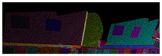
Figure 2. Segmentation plane point cloud.

3.3. Plane Simplification

Although most planar structures have been captured using our plane segmentation method, considerable redundancy still existed. We adopted a quadtree segmentation based on cluster fusion to simplify the planar feature. The advantage of this method is that the image can be efficiently partitioned into regular, square clustering regions. The plane simplification pipeline is shown in Figure 3. In the algorithm, different strategies were adopted in the boundary and interior of the plane. The boundary points were maintained to guarantee the overall distribution of the planar structure. Some new points were generated in the interior to reconstruct the characteristics of the planar structure.

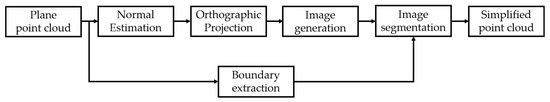
Figure 3. The pipeline of plane simplification.

3.3.1. Orthographic Projection

For each extracted plane point cloud $P{l}_i^B$, the plane normal $N{o}_i\left({\omega }_x,{\omega }_y,{\omega }_z\right)$ was estimated based on the least square. The rotation matrix $Rot$ in Equation (5) was obtained; then, the direction-corrected planar point cloud $P{l}_i^{dc}$ was acquired by rotating $P{l}_i^B$ with $Rot$. Subsequently, we obtained the projected point cloud $P{l}_i^{pr}$ in Equation (6).

$$Rot=I+{\rm K} \sin \theta + {{\rm K}}^2\left(1-\cos \theta \right), K=\left(\begin{array}{ccc}0& -{\omega }_z& {\omega }_y\\ {\omega }_z& 0& -{\omega }_x\\ -{\omega }_y& {\omega }_x& 0\end{array}\right)$$

(5)

$$P{l}_i^{pr}=\{p| p.x =q.x, p.y=q.y,p.z=0,q\in P{l}_i^{dc}\},$$

(6)

where $\theta$ is the angle between $N{o}_i$ and $\mathcal{Z}$ (0, 0, 1).

3.3.2. Image Generation

The boundary point cloud $Bd$ of $P{l}_i^{pr}$ was extracted using the alpha shape boundary method [61]. Subsequently, using Equation (7), we mapped $P{l}_i^{pr}$ to a grayscale image $I{g}_i$ using function $\Lambda$. Next, we set the height and width of $I{g}_i$ in Equation (8) to be equivalent to prepare for the subsequent segmentation.

$$\{\begin{array}{l} point cloud \stackrel{ \mathit{\Lambda } }{\to } Ig, Ig\stackrel{ {\mathit{\Lambda }}^{-}}{\to }point cloud\\ \mathit{\Lambda }: r= \frac{y^{max}- y}{res} , c= \frac{x - x^{min}}{res} \end{array}$$

(7)

$$w=h=\{2^s | 2^s>\max \left(b{r}_w, b{r}_h\right)> 2^{s-1}, s\in N\},$$

(8)

where x and y are the coordinates X and Y of each point in $P{l}_i^{pr}$, respectively; $r$ and $c$ are the row and column of each pixel in $Ig$, respectively; $res$ is the image pixel resolution; $b{r}_w$ and $b{r}_h$ are the width and height of the minimum bounding rectangle of $P{l}_i^{pr}$, respectively; and $w$ and $h$ are the width and height of $Ig$, respectively.

3.3.3. Quadtree Segmentation

The pixels in $I{g}_i$ are classified into exterior ($Ep)$, boundary ($Bp$), and interior ($Ip$). In Figure 4, the principle of quadtree segmentation is illustrated, where $I{g}_i$ is partitioned into four square regions each time. The segmentation process does not terminate until all elements are the same in each partitioned region. Subsequently, all $Bp$ and interior squares ($Is$) that contain $Ip$ are preserved. The four corners in $Bp$ and $Is$ are converted into point clouds $Bp{p}_i^S$ and $Is{p}_i^S$ through function ${\mathit{\Lambda }}^{-}$. Finally, for each $P{l}_i^B$, a simplified plane point cloud $P{l}_i^s$ comprising $Bp{p}_i^S$ and $Is{p}_i^S$ is obtained.

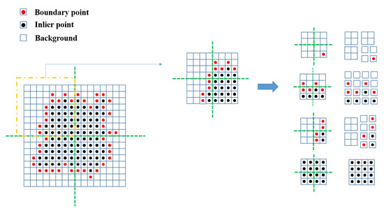
Figure 4. The quadtree segmentation based on cluster fusion.

The simplified planar point cloud is shown in Figure 5. The result (Figure 5b) shows the boundary points accurately. As shown in Figure 5c, the grayscale values for $Ep$, $Bp$, and $Ip$ in $I{g}_i$ were set to 0, 100, and 240, respectively, for distinction. For the planar simplified result (Figure 5d), the outline of the planar segments was preserved, and the interior redundant points were removed.

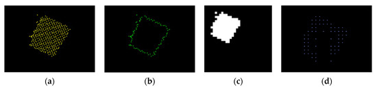
Figure 5. Simplification results of plane point cloud: (a) original plane point cloud, (b) boundary point cloud in green, (c) grayscale image, and (d) simplified plane point cloud ($P{l}_i^s$).

3.4. Feature Triangulation

After the planar simplification, we reconstructed the model representation of the planar feature using different triangulation strategies in the interior and boundary of each $P{l}_i^s$. In the interior, a simple triangulation was performed, in which two triangles were directly generated based on the four corners of $Is{p}_i^S$. At the boundary, a vertex-assignment triangulation (Figure 6) was performed, and four rules were proposed for the triangulation process.

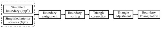
Figure 6. Flow chart of vertex-assignment triangulation.

3.4.1. Boundary Assignment

The proposed boundary triangulation uses $Bp{p}_i^S$ and $Is{p}_i^S$ as inputs and generates the feature triangulation. Figure 7 shows our proposed distance rule. Figure 7a shows two types of relative positions between the points and edges as well as the proposed distance rule for calculating the distance from a point to an edge. Figure 7b shows the calculation of the distances from $bp{p}_j$($bp{p}_j \in Bp{p}_i^S$) to the four edges in $is{p}_k\left(is{p}_k\in Is{p}_i^S\right)$. $e_m$, i.e., the edge with the minimum distance to $bp{p}_j$, was determined, and the corresponding minimum distance was regarded as the distance from $bp{p}_j$ to $is{p}_k$. Subsequently, $bp{p}_j$ was categorized into the collected point set $Ps$ of $e_m$. In Figure 7b, $d_1$ is the minimum distance and $e_1$ is the $e_m$. Finally, the $Ps$ for all edges of $is{p}_k$ was obtained.

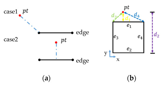
Figure 7. Distance rule: (a) two sorts of relative position between point and edge and (b) determination of the closest edge. $pt$ refers to a $bpp$ point. ${\mathrm{e}}_{1-4}$ represent four edges of $is{p}_k$. $d_{1-4}$ represent the distance from a $bpp$ point to four edge in $is{p}_k$.

3.4.2. Boundary Sorting

For the non-empty $Ps$ on one edge, the projection point ${\vartheta }_{pt}$ of $bp{p}_j$ on the corresponding edge was calculated. Figure 8 shows the proposed sorting for sorting the boundary points in each $Ps$. The sorting rule was based on the coordinates of ${\vartheta }_{pt}$. The x- or y-coordinates were utilized to sort the boundary points based on the direction of the edge. Y and X were selected for the vertical and horizontal directions, respectively.

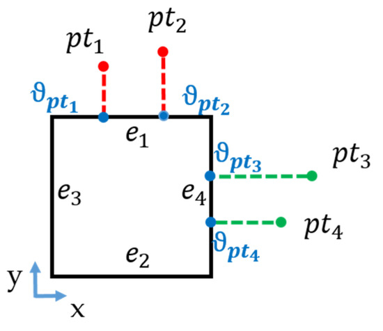
Figure 8. Sorting rule: ${\vartheta }_{p{t}_{1-4}}$ are the projection points. $p{t}_1$ and $p{t}_2$ are sorted according to the x coordinate of ${\vartheta }_{p{t}_1}$ and ${\vartheta }_{p{t}_2}$. $p{t}_3$ and $p{t}_4$ are sorted according to the y coordinate of ${\vartheta }_{p{t}_3}$ and ${\vartheta }_{p{t}_4}$.

3.4.3. Triangle Connection

After boundary sorting, we proposed a connection rule to construct the triangle preliminarily, as shown in Figure 9. For every non-empty $Ps$ point on one edge, we connected triangles through two neighbor boundary points. Four types of triangle connections were summarized based on the relative position between the edge and two neighbor points. In Figure 9, $p{t}_1$ and $p{t}_2$ represent two $bpp$ points. Type 1 (Figure 9a) involves two points outside the same side of the edge; type 2 (Figure 9b) involves one point inside the edge and another point outside the edge; type 3 (Figure 9c) involves two points inside the edge; and type 4 (Figure 9d) involves two points outside the different sides of the edge. In type 4, a midpoint between two boundary points is generated to assist the connection of triangles.

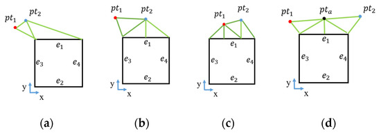
Figure 9. Connection rule: (a) type 1, (b) type 2, (c) type 3, and (d) type 4. $p{t}_a$ is the midpoint of two neighbor $bpp$ points.

3.4.4. Triangle Adjustment

After the preliminary triangle connection, some irrational triangles that intersect with other squares must be modified. Therefore, an adjustment rule was proposed to modify the inappropriate triangles, as shown in Figure 10. Figure 10a shows triangle ($l_1$, $l_2$, $e_4$) intersecting with square $S_2$. Figure 10b shows the original triangle modified as follows: First, the intersection edge $l_1$, intersection square $S_2$, and the edge to which it belonged ($e_4$) were determined. Subsequently, the projection point ${\vartheta }_{pt}$ on $e_4$ was calculated. Finally, the vertex closest to ${\vartheta }_{pt}$ in $S_2$ was selected, and a new triangle ($l_1$, $l_3, l_4$) was used to replace triangle ($l_1$, $l_2$, $e_4$).

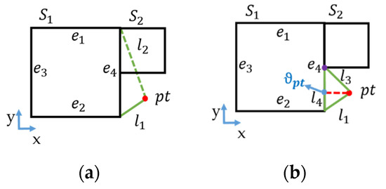
Figure 10. Adjustment rule: (a) triangle intersecting with square and (b) triangle after modification. $pt$ means a $bpp$ point. $S_{1-2}$ represent two interior squares. $l_{1-4}$ mean the edges of the triangle. ${\vartheta }_{pt}$ is the projection point. The purple point is the vertex point closest to ${\vartheta }_{pt}$ in $S_2$.

The feature triangulation of the planar point cloud is shown in Figure 11. In Figure 11a, every $bbp$ is connected to a certain edge of $isp$, and the relation between the boundary and interior in the plane is strengthened for each $P{l}_i^s$. The result visually preserves the outline of the planar feature. Interior triangulation using the simplified square corner significantly decreased the number of triangles. Subsequently, we constructed a triangulated FSM in all extracted planar point clouds $P{l}^B$. Our FSM in mesh form is shown in Figure 11b–d.

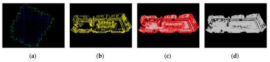
Figure 11. Feature triangulation: (a) triangulation of one planar point cloud, (b) all preserved vertices of triangulation, (c) the adjacency of the triangulation, and (d) the mesh model.

3.5. NSM

In robot navigation, an appropriate navigation map is necessary and favorable. Our NSM comprises an original planar point cloud $P{l}^B$ and a PAM. Compared with the existing NSM, the obstacles and passable area in our NSM are represented using points with coordinate dimension reduction, and the complex three-dimensional information is disregarded. Moreover, our NSM integrates $P{l}^B$, a structure with a unified feature. The extracted $P{l}^B$ can be regarded as a feature reference map in an indoor location based on a point cloud. The constructed PAM can serve as indoor navigation and path planning. As shown in Figure 12, the flow chart of the NSM construction comprises ground extraction and map construction. The method uses $R{p}^u$ and $P{l}^B$ as inputs and generates a hybrid NSM.

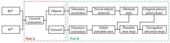
Figure 12. The flow chart of navigation structure map (NSM) construction.

3.5.1. Ground Extraction

The processing pipeline of the PAM is shown in Figure 13. The input comprises $P{l}^B$ and $R{p}^u$. In indoor scenes, typical assumptions include piecewise planar permanent structures and Manhattan world scenes in three orthogonal directions: two for the walls and one for the floors and ceilings [31]. The pipeline of the ground extraction included the following steps.

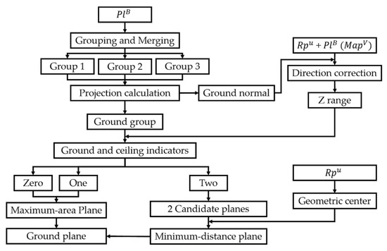
Figure 13. Pipeline of ground extraction.

(1)

Plane Grouping and Merging

$P{l}^B$ was grouped based on the normal direction to the plane and merged based on the distance expressed in Equation (9). Three dominant plane groups $gr{p}^i\left(i=0,1,2\right)$ were selected based on the plane quantity. Furthermore, the direction $di{r}_i$ of $gr{p}^i$ was determined using Equation (10).

$$d_{pl}=k_1\ast \frac{⟨p_s,n_t⟩ + d_t}{\sqrt{{\left(n_t\right)}_x^2+{\left(n_t\right)}_y^2+ {\left(n_t\right)}_z^2}}+k_2\ast \frac{⟨p_t,n_s⟩ + d_s}{\sqrt{{\left(n_s\right)}_x^2+{\left(n_s\right)}_y^2+ {\left(n_s\right)}_z^2}}$$

(9)

$$di{r}_i=\{nr{l}_i | j\stackrel{max}{\leftarrow }np\left(gr{p}_j^i\right), j=0,1,2\dots \mathrm{n}\left(gr{p}^i\right)\},$$

(10)

where $k_1$ and $k_2$ are two weight coefficients set to 0.5, $gr{p}_j^i$ is the jth plane in the ith plane group, $nrl$ is the normal to plane $gr{p}_j^i$, $np\left(gr{p}_j^i\right)$ is the point quantity of $gr{p}_j^i$, and $n\left(gr{p}^i\right)$ is the plane quantity of $gr{p}^i$.

(2)

Direction Correction

In Equation (11), the plane group containing the ground, $gr{p}^g$, was detected using the projection area. The correction matrix was obtained with $di{r}_g$, which is the direction of $gr{p}_g$, using Equation (5). The corrected point cloud $Ma{p}^C$ was obtained by rotating $Ma{p}^V$. Subsequently, the z-range ($z_{min}, z_{max}$) of $Ma{p}^C$ was calculated.

$$gr{p}_g=\{gr{p}_i | i\stackrel{max}{\leftarrow }are{a}^i,are{a}^i\stackrel{max}{\leftarrow }pa\left(gr{p}_j^i\right), i=0,1,2, j=0,1,\dots ,np\left(gr{p}^i\right)\},$$

(11)

where $pa\left(gr{p}_j^i\right)$ is a function to compute the projection area of the jth plane in $gr{p}_i$, the projection area is approximated using the area of the minimum bounding rectangle of the projection point cloud, $are{a}^i$ is the maximum projection area of the planes in $gr{p}_i$, and $np\left(gr{p}^i\right)$ is the plane quantity in the ith plane group.

(3)

Indicator Calculation

In Equation (12), the two z-ranges $\left(z_{min}^d, z_{min}^u\right)$ and $\left(z_{max}^d, z_{max}^u\right)$ were determined using scale parameter $\kappa$ and the z range ($z_{min}, z_{max}$). Two sets of planes, $se{t}^1$ and $se{t}^2$, for which the z coordinates were within $\left(z_{min}^d, z_{min}^u\right)$ and $\left(z_{max}^d, z_{max}^u\right)$, respectively, were selected from $gr{p}^g$. Subsequently, $p{l}_1^c$ and $p{l}_2^c$, two candidate planes with maximum areas, were extracted from $se{t}^1$ and $se{t}^2$, respectively. The ground and ceiling indicators were obtained using Equation (13). They comprised three states (0, 1, 2), where (a) state 0 indicates that neither the candidate ground nor ceiling is detected, (b) state 1 means that only one type is detected in the candidate ground and candidate ceiling, and (c) state 2 means that both the candidate ceiling and ground are detected. In states 0 and 1, the plane with the maximum area in $gr{p}^g$ is directly identified as the ground as we assume that the ceiling does not exist in this case and that the ground is the most significant plane. In state 2, the two selected candidate planes can be considered as the ground and ceiling. As both the ground and ceiling exist in the data, objects in the scene are closer to the ground than the ceiling. Furthermore, the $p{l}_k^c$ (k = 1, 2) that is closer to the geometric center in $R{p}^u$ is identified as the ground. Finally, the ground plane extraction results are shown in Figure 14.

$$\{\begin{array}{l}d= \kappa \ast \left({\mathrm{z}}_{max}- {\mathrm{z}}_{min} \right)\\ \left(z_{min}^d, z_{min}^u\right)=\left({\mathrm{z}}_{min}-d,{\mathrm{z}}_{min}+d\right)\\ \left(z_{max}^d, z_{max}^u\right)=\left({\mathrm{z}}_{max}-d,{\mathrm{z}}_{max}+d\right)\end{array}$$

(12)

$$indicator=\{ \begin{array}{l}0,\nexists z_i^p\in \left(z_{min}^d, z_{min}^u\right)and \nexists z_j^p\in \left(z_{max}^d, z_{max}^u\right)\\ 1, \exists z_i^p\in (z_{min}^d,z_{min}^u)or \exists z_i^p\in (z_{max}^d,z_{max}^u)\\ 2, \nexists z_i^p\in \left(z_{min}^d, z_{min}^u\right)and \nexists z_j^p\in \left(z_{max}^d, z_{max}^u\right), \end{array}$$

(13)

where $z_i^p$ is the average z coordinate of the ith plane in $gr{p}^g$, and i and j are the ith and jth planes, respectively, in $gr{p}^g$.

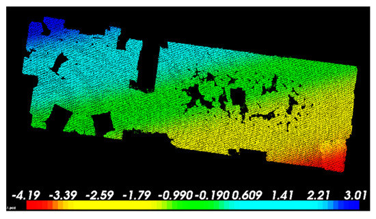
Figure 14. Ground extraction result.

3.5.2. Map Construction

(1)

Initial Passage Area Construction

$Ma{p}^V$ was segregated into a ground plane and space obstacles after ground extraction. They were corrected by aligning the ground with the XOY plane, and the direction-corrected ground is shown in Figure 15a. As shown in Figure 15b, Euclidean clustering was adopted to remove trivial points in the spatial obstacles. All areas were passable when no objects were above the ground. The holes in the ground were filled with contour filling in the image. As shown in Figure 15c, a binary image $I_{grd}$ based on the ground was generated based on function $\Lambda$ in Equation (7). As shown in Figure 15d, the contours of the ground were extracted and filled, and then, the initial passable area in the image format was constructed.

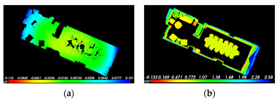
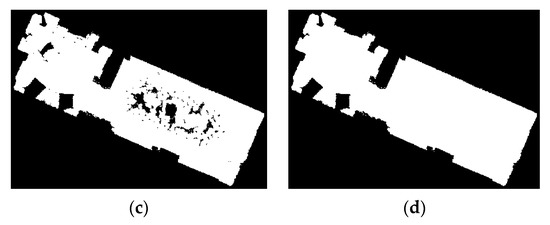
Figure 15. Initial passable area map (PAM) and space obstacles: (a) direction-corrected ground, (b) space obstacles, (c) binary image ($I_{grd}$), and (d) initial PAM in image format.

(2)

PAM Construction

Because the volume of the indoor robot varied, the obstacle maps within different heights were constructed. Several obstacle maps $I_{obj}$ with different heights in the image format were generated. Subsequently, $I_{pass}$, the PAM in image format, was constructed within different heights based on Equation (14). Next, a PAM in the point cloud format was generated using ${\Lambda }^{-}$.

$$I_{pass}= {\complement }_{I_{grd}}^{I_{grd} {\displaystyle \cap } I_{obj}}$$

(14)

We constructed a PAM for five height ranges (0–0.4, 0–0.8, 0–1.2, 0–1.6, and 0–2.0). A map with height range (0–1.2) is shown in Figure 16. Different areas are shown in different colors (green and red represent the passable and obstacle areas, respectively). The PAM can visually depict the position of the objects.

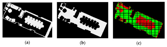
Figure 16. PAM with height range (0–1.2): (a) the obstacle map in binary format, (b) PAM in image format, and (c) PAM in point cloud format.

(3).

Construction of NSM

The NSM comprises the original planar point cloud described in Section 3.2 and the PAM presented Section 3.5. In robot navigation, we typically construct a global feature reference map in advance. Subsequently, the features collected in real time are exploited to match those extracted in the global feature reference map to accomplish navigation. In our study, the extracted feature is a planar structure. The PAM can be used to indicate the passable area for path planning.

4. Experiment

4.1. Platform and Data Description

As shown in Figure 17, two types of datasets were utilized in our experiment. Two simulation datasets (Figure 17a,b) were used to evaluate the performance of our proposed two-stage plane segmentation method. Four real datasets (Figure 17c–f) were used in our ISE method test. We obtained real datasets 1–3 from Park et al. [62], whereas we collected real dataset 4 using a Faro scanner. All four real datasets were collected in the connected indoor space because our method was intended for representing the indoor structure, not the space partition. Real dataset 1 was a boardroom dataset comprising a conference space and rest space. It was filled with cluttered chairs, closets, and wall structures. Real dataset 2 was an apartment dataset comprising more rooms, and real dataset 3 was a bedroom dataset with a relatively small space. Real dataset 4 was a neat exhibition room dataset with excellent planar structures. Real datasets 1–3 comprised the ground but not the ceiling; however, both structures existed in real dataset 4. A laptop with an Intel Core i7-5500U CPU @2.40 GHz/2.39 GHz and 8.0 GB of RAM was applied in our experiment.

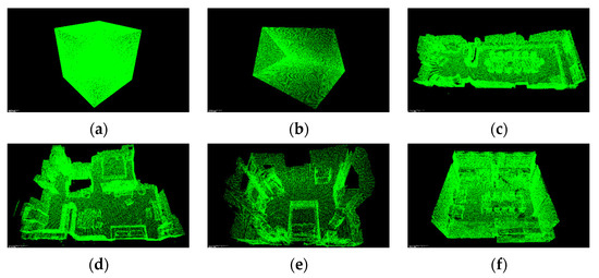
Figure 17. Experimental datasets: (a) simulation dataset 1, (b) simulation dataset 2, (c) real dataset 1, (d) real dataset 2, (e) real dataset 3, and (f) real dataset 4.

4.2. Parameter Setting

The parameter settings for our ISE method are shown in Table 1. The parameters were classified based on to the stages of our method. (a) In preprocessing, $n{k}_1$ and $r$ were empirically determined based on the point cloud density to process the raw point cloud. (b) In FSM construction, the parameters were set to improve the accuracy of the extracted structure and to preserve the structural details of the FSM. Figure 18 shows some of the parameters used in detail;${\delta }_1$ and ${\delta }_2$ were approximated using Equations (15) and (16), respectively. (c) In NSM construction, the parameters used were mainly for ground extraction and PAM construction. The parameter setting in our method offers two advantages: (1) it is applicable to typical indoor dense point clouds and is independent of the scale of the scene, and (2) small changes in the parameters do not significantly affect the overall experimental result.

Table 1. Overview of parameters in proposed method.

Stage		Parameter	Value
Preprocessing	Statistical filtering	Neighbor points $n{k}_1$	50
	Voxel filtering	Voxel size $r$/m	0.02
FSM construction	Plane segmentation	Angle threshold ${\theta }_1$/°	3
		Distance threshold ${\delta }_1$/m	0.03
		Distance threshold ${\delta }_2$/m	0.004
		Point quantity threshold ${\zeta }_1$	100
	Plane simplification	Neighbor points $n{k}_2$	50
		Image pixel resolution ${\partial }_1/\mathrm{m}$	0.03
NSM construction	Ground extraction	Plane group angle threshold ${\theta }_2/°$	10
		Plane merge distance threshold ${\delta }_3/\mathrm{m}$	0.05
		Indicator ratio $\kappa$	0.2
	Map construction	Minimum point number of cluster $\nu$	70
		Image pixel resolution ${\partial }_2/\mathrm{m}$	0.03

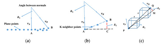
Figure 18. Parameter setting description: (a) region growing neighborhood, (b)${\delta }_1$, and (c) ${\delta }_2$.

$${\delta }_1\approx BC= r\ast k\ast {\theta }_1$$

(15)

$${\delta }_2\approx 2\sqrt{3}r\ast {\theta }_1$$

(16)

4.3. Experimental Results

The experimental results of four real datasets are shown in this section. The results of our proposed ISE method included an FSM and an NSM. The FSM was a mesh model generated from a plane feature. The NSM comprised a PAM and the original planar point cloud, where the PAM mainly served as obstacle indication and path planning, whereas the original planar feature point cloud was considered the localization reference. Moreover, our PAM was represented in two formats: point cloud and binary image. Some quantitative statistics of the results are listed in Table 2.

Table 2. Statistical indicators of four real datasets.

Real Dataset	Number of Points in Original Dataset	Number of Planar Segments	Number of Patches in Mesh
1. Boardroom	9,268,856	563	142,055
2. Apartment	8,560,872	384	130,924
3. Bedroom	5,318,546	339	94,627
4. Reading room	67,906,207	377	127,563

4.3.1. Real Dataset 1

Real dataset 1 was a boardroom dataset with a relatively large connection space and some clustered objects. It included some salient plane features such as a ground, conference table, wall, and cupboard. A total of 142,055 patches were constructed in the FSM (Figure 19a). The original planar point cloud (Figure 19b) contained 563 planes. The constructed PAM is shown in Figure 19c. Our NSM was composed of the original planar point cloud and the PAM. A similar display form for the NSM of real datasets 2–4 is shown in Figure 20, Figure 21 and Figure 22, respectively. The PAM between height ranges 1 and 2 differed significantly, and the change among PAMs 2–5 was insignificant. The constructed PAM conformed visually to the indoor layout.

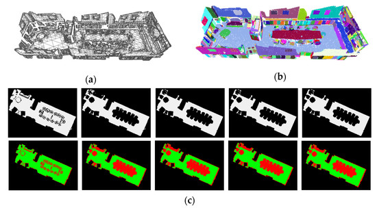
Figure 19. Indoor structure extraction (ISE) result of real dataset 1: (a) feature structure map (FSM) result, (b) original planar point cloud, and (c) PAM.

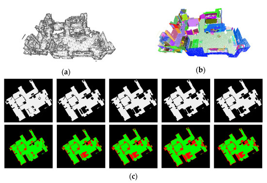
Figure 20. ISE result of real dataset 2: (a) FSM result, (b) original planar point cloud, and (c) PAM.

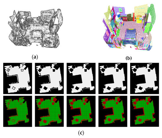
Figure 21. ISE result of real dataset 3: (a) FSM result, (b) original planar point cloud, and (c) PAM.

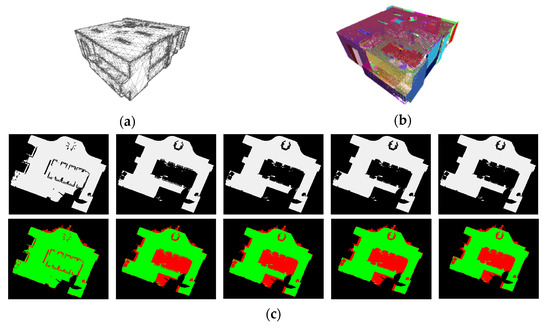
Figure 22. ISE result of real dataset 4: (a) FSM result, (b) original planar point cloud, and (c) PAM.

4.3.2. Real Dataset 2

Real dataset 2 was an apartment dataset comprising four connected room spaces and plenty of wall structures. Compared with real dataset 1, the wall structure was more dominant. A total of 130,924 patches were constructed in the FSM (Figure 20a). The original planar point cloud (Figure 20b) contained 384 planes. Although the number of extracted planes was small, those planes had a larger area and higher integrity. As the height range increased, the bed appeared as an obstacle in the PAM, as shown in Figure 20c.

4.3.3. Real Dataset 3

Dataset 3 was a small-area bedroom dataset with one connected room space. Most of the plane features were small planar segments from the ground, wall, wardrobe, and bed. The FSM (Figure 21a) contained 94,627 patches. The original planar point cloud (Figure 21b) contained 339 planes. To accommodate the purpose of the bedroom, few obstacles were present, and the constructed PAM (Figure 21c) did not differ significantly.

4.3.4. Real Dataset 4

Dataset 4 was a reading room dataset that we collected using a Faro scanner. The merged dataset contained dense points, and the salient plane features were similar to those of real dataset 1. The most obvious difference between this dataset and real datasets 1–3 was that the former contained a large ceiling. The constructed mesh model (Figure 22a) contained 127,563 patches. The original planar point cloud (Figure 22b) contained 377 planes. As shown in Figure 22c, the two most significant obstacles in the PAM were the conference table and exhibition stand.

5. Discussion

5.1. Performance of Plane Segmentation

As show in Figure 23, both the simulation and real datasets were used to compare the plane segmentation performances between the proposed two-staged region growing and traditional region growing algorithm (TRG). Two simulation datasets (Figure 17a,b) were used for the quantitative evaluation. Simulation dataset 1 was a cube with a 0.01-m point resolution and 90,000 points on each surface. Simulation dataset 2 was a triangular prism with a 0.02-m point resolution, where each rectangle and triangle comprised 60,000 and 17,421 points, respectively. Part of real dataset 1 was used to compare the results visually.

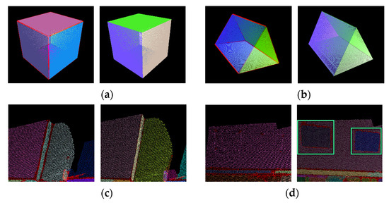
Figure 23. Comparison of plane segmentation: (a) simulation dataset 1, (b) simulation dataset 2, and (c,d) part of real dataset 1. Red points mean unclassified points. Other color points mean different planes. In each panel, the left image is the result from traditional region growing (TRG) and the right image is the result from our method.

As shown in Figure 23, some unclassified red points appeared near the boundary or intersection of the planes in the TRG results. However, the number of unclassified points reduced visually in the results obtained using our method. Moreover, some concave and convex structures on the wall (green rectangle in Figure 23d) were not identified in the TRG but were captured successfully using our method.

The recall of the extracted plane result was estimated using Equation (17). The quantitative performance of plane segmentation for the two simulation datasets is shown in Table 3. The integrity of all the planes increased, and the average planar integrity of the two simulation datasets in our method was higher than those in the TRG, i.e., approximately 4% for the square and 6% for the triangular prism.

$$Recall = \frac{Point{s}_{recon} {\displaystyle \cap } Point{s}_{true}}{Point{s}_{true}},$$

(17)

where $Point{s}_{recon}$ are the extracted plane points and $Point{s}_{true}$ are the real plane points.

Table 3. Performance of plane segmentation for simulation datasets.

Surface Id	Simulation Dataset 1 (Square)			Simulation Dataset 2 (Triangular Prism)
	Point Number	Point Number/ (Recall/%)		Point Number	Point Number/ (Recall/%)
	Original Dataset	TRG	Our method	Original Dataset	TRG/	Our Method
1	90,000	85,849(95.39)	89,920(99.91)	60,000	56,154(93.59)	59,542(99.24)
2	90,000	85,849(95.39)	89,880(99.87)	60,000	56,155(93.59)	59,980(99.97)
3	90,000	85,849(95.39)	89,850(99.83)	60,000	56,155(93.59)	59,274(98.79)
4	90,000	86,436(96.04)	89,401(99.33)	17,421	15,826(90.84)	16,969(97.41)
5	90,000	86,436(96.04)	89,401(99.33)	17,421	16,078(92.29)	17,162(98.51)
6	90,000	86,436(96.04)	89,401(99.33)	-	-	-
Sum	540,000	516,855(95.71)	537,853(99.60)	214,842	200,368(93.26)	212,927(99.11)

5.2. Triangulation Performance

The constructed FSM was compared with that obtained using the traditional greedy projection triangulation (GPT) for further evaluation. In Equations (18)–(20), three statistical metrics, area mean value ($Mean$), area standard deviation ($Stdev$), and area range ($Range$) for the patches in the mesh model, were selected to analyze the algorithm performance. These geometric attributes included the area concentration trend ($Mean$), area variation intensity ($Stdev$), and area variation range ($Range$) of the triangular patches in the FSM. The large-volume indoor data differed from the airborne terrestrial point cloud data; it contained plenty of large-area artificial surfaces such as walls, cylinders, and related surfaces. However, a few small obstacles were present for robot localization. Therefore, the $Mean$ of the triangular surface area was relatively larger, and more significantly, $Stdev$ and $Range$ were larger. The three statistical metrics for an excellent ISE based on the point cloud should be relatively large, and they can better quantify the geometric attributes for the constructed FSM compared with the traditional data reduction ratio [25].

Moreover, the quantity of triangular patches ($Quantity$) was used in the evaluation. A comparison of the four statistics is shown in Figure 24. As shown, the $Mean$, $Stdev$, and $Range$ of our method were significantly higher, whereas the $Quantity$ of our method was lower than that of the GPT. Our FSM attempted to capture the outline information describing the distribution of the structure and disregarded some redundant feature information. Hence, using a few large patches inside the plane and massive small patches around the boundary can not only reduce the data memory but also ensure the structure details.

$$Mean=\frac{{\sum }_i^{N}Ar\left(f_i\right) }{N}$$

(18)

$$Stdev=\frac{{\sum }_i^N{\left(Ar\left(f_i\right)- Mean\right)}^2 }{N-1}$$

(19)

$$Range= Ar{\left(f_i\right)}^{max}- Ar{\left(f_i\right)}^{min},$$

(20)

where N is the number of triangular patches in the FSM; $f_i$ is the ith triangular patch; $Ar\left(f_i\right)$ is the area of $f_i$; and $Ar{\left(f_i\right)}^{max}$ and $Ar{\left(f_i\right)}^{min}$ are the maximum and minimum areas of $f_i$ respectively.

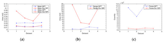
Figure 24. Statistics of patches in the mesh model: (a) $Mean$ and $Stdev$, (b) $Range$, and (c) $Quantity$. The $Mean$ and $Stdev$ from greedy projection triangulation (GPT) were enlarged by 100 times for visual display effect.

Compared with the traditional GPT, our method processed the boundary better, improved the integrity of the planar structure, and enhanced the recall of feature segmentation. As our method can successfully capture the details of the scene structure, ISE was more robust and the appearance of the FSM was more exquisite.

6. Conclusions

Herein, we proposed a novel ISE method based on a dense unstructured point cloud that can automatically reconstruct an FSM based on a planar structure, resulting in a robust and exquisite FSM. Compared with the TRG method, our two-stage region growing method demonstrated a higher integrity of the planes. Automation of the process was improved through a logical parameter setting. The quadtree segmentation based on cluster fusion reduced redundancy. The proposed vertex assignment triangulation preserved the compact structure information around the boundary of the plane compared with GPT. The generated mesh can be applied to CAD or other software. The constructed mesh provides several functions: (1) indoor reconstruction—for some indoor complex scenes, the indoor structures should be analyzed; (2) structural repair—it strengthens the representation of the boundary feature of the structure and can serve as a basic model to preliminarily repair indoor structures; and (3) reduction in data memory—using the quadtree segmentation method, the structure of the plane point cloud can be represented with less data memory. Our ISE method can automatically reconstruct a novel form of NSM comprising the original planar point cloud and a PAM. It can identify the ground effectively in a clustered indoor scene and is not subject to the scanning coordinate, i.e., the XOY plane in the coordinate system does not need to be horizontal. In the PAM, the location of the obstacles within different heights was indicated using the points after coordinate dimension reduction. Moreover, the hybrid form of the ISE results rendered our method more applicable than the traditional single form of the ISE result.

In this study, we discovered a few challenges in the real indoor scenes: (1) our method was performed based on a dense point cloud collected using a 3D scanner or aligned via several scans. Our method may be subject to the accuracy of the original scan data; (2) the NSM result can serve as a reference feature map, and the efficiency of the construction process before real-time robot navigation can be improved; (3) movable objects in the indoor spaces must be considered; and (4) navigation may be applied to larger spaces with more rooms and corridors.

In future studies, several issues must be addressed, as follows: (1) Our ISE method only exploited the plane structure to construct the FSM; however, many types of structures exist in indoor scenes. Therefore, an FSM based on more types of structures must be investigated. (2) We should apply our NSM to real-time robot navigation using real-time perception systems in future studies. (3) A learning semantic annotation method may be investigated to label and locate the indoor structure to verify whether the constructed map results must be updated. Movable and non-movable objects in the indoor spaces must be discriminated and provided with different weights during navigation. (4) An FSS framework may be required to facilitate the use of our method for indoor robot navigation in larger spaces containing more rooms and corridors.

References

- Österbring, M.; Thuvander, L.; Mata, É.; Wallbaum, H. Stakeholder Specific Multi-Scale Spatial Representation of Urban Building-Stocks. ISPRS Int. J. Geo-Inf. 2018, 7, 173. [Google Scholar] [CrossRef]
- Lehtola, V.V.; Kaartinen, H.; Nüchter, A.; Kaijaluoto, R.; Kukko, A.; Litkey, P.; Honkavaara, E.; Rosnell, T.; Vaaja, M.T.; Virtanen, J.-P.; et al. Comparison of the Selected State-Of-The-Art 3D Indoor Scanning and Point Cloud Generation Methods. Remote Sens. 2017, 9, 796. [Google Scholar] [CrossRef]
- Piccinni, G.; Avitabile, G.; Coviello, G.; Talarico, C. Modeling of a Re-Configurable Indoor Positioning System Based on Software Defined Radio Architecture. In Proceedings of the 2018 New Generation of CAS (NGCAS), Valletta, Malta, 20–23 November 2018; pp. 174–177. [Google Scholar] [CrossRef]
- Davis, J.; Marschner, S.R.; Garr, M.; Levoy, M. Filling holes in complex surfaces using volumetric diffusion. In Proceedings of the Symposium on 3D Data Processing, Visualization, and Transmission (3DPVT), Padova, Italy, 19–21 June 2002; pp. 428–441. [Google Scholar] [CrossRef]
- Kim, C.; Moon, H.; Lee, W. Data management framework of drone-based 3D model reconstruction of disaster site. In Proceedings of the 23rd International Archives of the Photogrammetry, Remote Sensing and Spatial Information Sciences Congress (ISPRS), Prague, Czech Republic, 12–19 July 2016; pp. 31–33. [Google Scholar] [CrossRef]
- Samad, S.; Lim, S.; Sara, S. Implementation of Rapid As-built Building Information Modeling Using Mobile LiDAR. In Proceedings of the 2014 Construction Research Congress (CRC): Construction in a Global Network, Atlanta, GA, USA, 19–21 May 2014; pp. 209–218. [Google Scholar] [CrossRef]
- Chiabrando, F.; Di Pietra, V.; Lingua, A.; Cho, Y.; Jeon, J. An Original Application of Image Recognition Based Location in Complex Indoor Environments. ISPRS Int. J. Geo-Inf. 2017, 6, 56. [Google Scholar] [CrossRef]
- Gupta, T.; Li, H. Indoor mapping for smart cities—An affordable approach: Using Kinect Sensor and ZED stereo camera. In Proceedings of the 2017 International Conference on Indoor Positioning and Indoor Navigation (IPIN), Sapporo, Japan, 18–21 September 2017; pp. 1–8. [Google Scholar] [CrossRef]
- Lan, Z.; Yew, Z.J.; Lee, G.H. Robust Point Cloud Based Reconstruction of Large-Scale Outdoor Scenes. In Proceedings of the 2019 IEEE/CVF Conference on Computer Vision and Pattern Recognition (CVPR), Long Beach, CA, USA, 15–20 June 2019; pp. 9682–9690. [Google Scholar] [CrossRef]
- Skuratovskyi, S.; Gorovyi, I.; Vovk, V.; Sharapov, D. Outdoor Mapping Framework: From Images to 3D Model. In Proceedings of the 2019 Signal Processing Symposium (SPSympo), Krakow, Poland, 17–19 September 2019; pp. 296–399. [Google Scholar] [CrossRef]
- Debaditya, A.; Kourosh, K.; Stephan, W. BIM-PoseNet: Indoor camera localisation using a 3D indoor model and deep learning from synthetic images. ISPRS J. Photogramm. Remote Sens. 2019, 150, 245–258. [Google Scholar] [CrossRef]
- Liu, M.; Zhang, K.; Zhu, J.; Wang, J.; Guo, J.; Guo, Y. Data-Driven Indoor Scene Modeling from a Single Color Image with Iterative Object Segmentation and Model Retrieval. IEEE Trans. Vis. Comput. Graph. 2020, 26, 1702–1715. [Google Scholar] [CrossRef] [PubMed]
- Liu, M.; Zhang, Y.; He, J.; Guo, J.; Guo, Y. Image-Based 3D Model Retrieval for Indoor Scenes by Simulating Scene Context. In Proceedings of the 25th IEEE International Conference on Image Processing (ICIP), Athens, Greece, 7–10 October 2018; pp. 3658–3662. [Google Scholar] [CrossRef]
- Tran, H.; Khoshelham, K. Procedural Reconstruction of 3D Indoor Models from Lidar Data Using Reversible Jump Markov Chain Monte Carlo. Remote Sens. 2020, 12, 838. [Google Scholar] [CrossRef]
- Pang, M.; Luo, C.; Mei, X.; Lin, H. Acceleration of Shadowing Detection with Octree and Improved Specular Model for Indoor Propagation Using Point Cloud Data. In Proceedings of the 2018 IEEE International Conference on Computational Electromagnetics (ICCEM), Chengdu, China, 26–28 March 2018; pp. 1–3. [Google Scholar] [CrossRef]
- Kim, B.K. Indoor localization and point cloud generation for building interior modeling. In Proceedings of the 2013 IEEE RO-MAN, Gyeongju, Korea, 26–29 August 2013; pp. 186–191. [Google Scholar] [CrossRef]
- Poux, F.; Neuville, R.; Nys, G.-A.; Billen, R. 3D Point Cloud Semantic Modelling: Integrated Framework for Indoor Spaces and Furniture. Remote Sens. 2018, 10, 1412. [Google Scholar] [CrossRef]
- Díaz-Vilariño, L.; Martínez-Sánchez, J.; Lagüela, S.; Armesto, J.; Khoshelham, K. Door recognition in cluttered building interiors using imagery and lidar data. In Proceedings of the ISPRS Technical Commission V Symposium, Riva del Garda, Italy, 23–25 June 2014; pp. 203–209. [Google Scholar] [CrossRef]
- Dumitru, R.-C.; Nüchter, A. Interior reconstruction using the 3D Hough transform. In Proceedings of the 3D Virtual Reconstruction and Visualization of Complex Architectures (3D-ARCH), Trento, Italy, 25–26 February 2013; pp. 65–72. [Google Scholar]
- Li, J.; He, X.; Li, J. 2D LiDAR and camera fusion in 3D modeling of indoor environment. In Proceedings of the NAECON 2015—IEEE National Aerospace and Electronics Conference, Dayton, OH, USA, 15–19 June 2015; pp. 379–383. [Google Scholar] [CrossRef]
- Yang, L.; Cheng, H.; Su, J.; Li, X. Pixel-to-Model Distance for Robust Background Reconstruction. IEEE Trans. Circuits Syst. Video Technol. 2019, 26, 903–916. [Google Scholar] [CrossRef]
- Pollefeys, M.; Nister, M.; Frahm, J.M.; Akbarzadeh, A.; Mordohai, P.; Clipp, B.; Engels, C.; Gallup, D.; Kim, S.J.; Merrell, P.; et al. Detailed real-time urban 3D reconstruction from video. Int. J. Comput. Vis. 2008, 78, 143–167. [Google Scholar] [CrossRef]
- Wang, H.; Wang, J.; Wang, L. Online Reconstruction of Indoor Scenes from RGB-D Streams. In Proceedings of the 2016 IEEE Conference on Computer Vision and Pattern Recognition (CVPR), Las Vegas, NV, USA, 27–30 June 2016; pp. 3271–3279. [Google Scholar] [CrossRef]
- Ma, L.; Whelan, T.; Bondarev, E.; de With, P.H.N.; McDonald, J. Planar simplification and texturing of dense point cloud maps. In Proceedings of the 2013 European Conference on Mobile Robots, Barcelona, Spain, 25–27 September 2013; pp. 164–171. [Google Scholar] [CrossRef]
- Feichter, S.; Hlavacs, H. Planar Simplification of Indoor Point-Cloud Environments. In Proceedings of the 2018 IEEE International Conference on Artificial Intelligence and Virtual Reality (AIVR), Taichung, Taiwan, 10–12 December 2018; pp. 274–281. [Google Scholar] [CrossRef]
- Adan, A.; Huber, D. 3D Reconstruction of Interior Wall Surfaces under Occlusion and Clutter. In Proceedings of the 2011 International Conference on 3D Imaging, Modeling, Processing, Visualization and Transmission (3DIMPVT), Hangzhou, China, 16–19 May 2011; pp. 275–281. [Google Scholar] [CrossRef]
- Oesau, S.; Lafarge, F.; Alliez, P. Indoor Scene Reconstruction using Feature Sensitive Primitive Extraction and Graph-cut. ISPRS J. Photogramm. Remote Sens. 2014, 90, 68–82. [Google Scholar] [CrossRef]
- Shui, W.; Liu, J.; Ren, P.; Maddock, S.; Zhou, M. Automatic planar shape segmentation from indoor point clouds. In Proceedings of the 15th ACM SIGGRAPH Conference on Virtual-Reality Continuum and Its Applications in Industry, VRCAI, Zhuhai, China, 3–4 December 2016; pp. 363–372. [Google Scholar] [CrossRef]
- Georgios-Tsampikos, M.; Renato, P. Bayesian graph-cut optimization for wall surfaces reconstruction in indoor environments. Vis. Comput. 2017, 33, 1347–1355. [Google Scholar] [CrossRef]
- Zhou, K.; Gorte, B.; Zlatanova, S. Exploring Regularities for improving façade reconstruction from point clouds. In Proceedings of the 23rd International Archives of the Photogrammetry, Remote Sensing and Spatial Information Sciences Congress (ISPRS), Prague, Czech Republic, 12–19 July 2016; pp. 749–755. [Google Scholar] [CrossRef]
- Ma, L.; Favier, R.; Do, L.; Bondarev, E.; de With, P.H.N. Plane segmentation and decimation of point clouds for 3D environment reconstruction. In Proceedings of the 2013 IEEE 10th Consumer Communications and Networking Conference (CCNC), Las Vegas, NV, USA, 11–14 January 2013; pp. 43–49. [Google Scholar] [CrossRef]
- Turner, E.; Zakhor, A. Watertight Planar Surface Meshing of Indoor Point-Clouds with Voxel Carving. In Proceedings of the 2013 International Conference on 3D Vision, Seattle, WA, USA, 29 June–1 July 2013; pp. 41–48. [Google Scholar] [CrossRef]
- Dimitrov, A.; Golparvar-Fard, M. Segmentation of building point cloud models including detailed architectural/structural features and MEP systems. Autom. Constr. 2015, 51, 32–45. [Google Scholar] [CrossRef]
- Poux, F.; Billen, R. Voxel-based 3D point cloud semantic segmentation: Unsupervised geometric and relationship featuring vs deep learning methods. ISPRS Int. J. Geo-Inf. 2019, 8, 213. [Google Scholar] [CrossRef]
- Papon, J.; Abramov, A.; Schoeler, M.; Worgotter, F. Voxel cloud connectivity segmentation—Supervoxels for point clouds. In Proceedings of the 2013 IEEE Conference on Computer Vision and Pattern Recognition (CVPR), Portland, OR, USA, 23–28 June 2013; pp. 2027–2034. [Google Scholar] [CrossRef]
- Vo, A.V.; Truong-Hong, L.; Laefer, D.F.; Bertolotto, M. Octree-based region growing for point cloud segmentation. ISPRS J. Photogramm. Remote Sens. 2015, 104, 88–100. [Google Scholar] [CrossRef]
- Armeni, I.; Sener, O.; Zamir, A.R.; Jiang, H.; Brilakis, I.; Fischer, M.; Savarese, S. 3D Semantic Parsing of Large-Scale Indoor Spaces. In Proceedings of the 2016 IEEE Conference on Computer Vision and Pattern Recognition (CVPR), Las Vegas, NV, USA, 27–30 June 2016; pp. 1534–1543. [Google Scholar] [CrossRef]
- Ochmann, S.; Vock, R.; Wessel, R.; Tamke, M.; Klein, R. Automatic generation of structural building descriptions from 3D point cloud scans. In Proceedings of the 9th International Conference on Computer Graphics Theory and Applications, Lisbon, Portugal, 5–8 January 2014; pp. 120–127. Available online: https://cg.cs.uni-bonn.de/aigaion2root/attachments/GRAPP_2014_54_CR.pdf (accessed on 17 June 2020).
- Tchuinkou Kwadjo, D.; Tchinda, N.; Bobda, C.; Menadjou, N.; Fotsing, C.; Nziengam, N. From PC2BIM: Automatic Model generation from Indoor Point Cloud. In Proceedings of the 13th International Conference on Distributed Smart Cameras, Trento, Italy, 9–11 September 2019; pp. 1–6. [Google Scholar] [CrossRef]
- Yang, F.; Li, L.; Su, F.; Li, D.; Zhu, H.; Ying, S.; Zuo, X.; Tang, L. Semantic decomposition and recognition of indoor spaces with structural constraints for 3D indoor modelling. Autom. Constr. 2019, 106, 319–339. [Google Scholar] [CrossRef]
- Shi, W.; Ahmed, W.; Li, N.; Fan, W.; Xiang, H.; Wang, M. Semantic Geometric Modelling of Unstructured Indoor Point Cloud. ISPRS Int. J. Geo-Inf. 2019, 8, 9. [Google Scholar] [CrossRef]
- Wang, C.; Hou, S.; Wen, C.; Gong, Z.; Li, Q.; Sun, X.; Li, J. Semantic line framework-based indoor building modeling using backpacked laser scanning point cloud. ISPRS J. Photogramm. Remote Sens. 2018, 143, 150–166. [Google Scholar] [CrossRef]
- Xiong, X.; Huber, D. Using Context to Create Semantic 3D Models of Indoor Environments. In Proceedings of the 2010 21st British Machine Vision Conference, Aberystwyth, Wales, UK, 31 August–3 September 2010; pp. 45.1–45.11. [Google Scholar] [CrossRef]
- Cui, Y.; Li, Q.; Yang, B.; Xiao, W.; Chen, C.; Dong, Z. Automatic 3-D Reconstruction of Indoor Environment With Mobile Laser Scanning Point Clouds. IEEE J. Sel. Top. Appl. Earth Obs. Remote Sens. 2019, 12, 3117–3130. [Google Scholar] [CrossRef]
- Xiong, X.; Adan, A.; Akinci, B.; Huber, D. Automatic Creation of Semantically Rich 3D Building Models from Laser Scanner Data. Autom. Constr. 2013, 31, 325–337. [Google Scholar] [CrossRef]
- Yang, L.; Worboys, M. Generation of navigation graphs for indoor space. Int. J. Geogr. Inf. Sci. 2015, 29, 1737–1756. [Google Scholar] [CrossRef]
- Brawn, G.; Nagel, C.; Zlatanova, S.; Kolbe, T. Modelling 3D Topographic Space against Indoor Navigation Requirements. In Proceedings of the 7th International Workshop on 3D Geoinformation, Quebec City, QC, Canada, 16–17 May 2012; pp. 1–22. [Google Scholar] [CrossRef]
- Nikoohemat, S.; Diakité, A.; Zlatanova, S.; Vosselman, G. Indoor 3D Modeling and Flexible Space Subdivision from Point Clouds. In Proceedings of the 4th ISPRS Geospatial Week, Enschede, The Netherlands, 10–14 June 2019; pp. 285–292. [Google Scholar] [CrossRef]
- Diakité, A.A.; Zlatanova, S. Spatial subdivision of complex indoor environments for 3D indoor navigation. Int. J. Geogr. Inf. Sci. 2018, 32, 213–235. [Google Scholar] [CrossRef]
- Zlatanova, S.; Liu, L.; Sithole, G. A conceptual framework of space subdivision for indoor navigation. In Proceedings of the 5th ACM SIGSPATIAL International Workshop on Indoor SpatialAwareness, Orlando, FL, USA, 5 November 2013; pp. 37–41. [Google Scholar] [CrossRef]
- Taneja, S.; Akinci, B.; Garrett, J.; Soibelman, L. Algorithms for automated generation of navigation models from building information models to support indoor map-matching. Autom. Constr. 2016, 61, 24–41. [Google Scholar] [CrossRef]
- Flikweert, P.; Peters, R.; Díaz-Vilariño, L.; Voûte, R.; Staats, B. Automatic Extraction of A Navigation Graph Intended for IndoorGML From An Indoor Point Cloud. In Proceedings of the 4th ISPRS Geospatial Week, Enschede, The Netherlands, 10–14 June 2019; pp. 271–278. [Google Scholar] [CrossRef]
- Boguslawski, P.; Mahdjoubi, L.; Zverovich, V.; Fadli, F. Automated construction of variable density navigable networks in a 3D indoor environment for emergency response. Autom. Constr. 2016, 72, 115–128. [Google Scholar] [CrossRef]
- Li, F.; Wang, H.; Akwensi, P.H.; Kang, Z. Construction of Obstacle Element Map Based on Indoor Scene Recognition. In Proceedings of the 4th ISPRS Geospatial Week, Enschede, The Netherland, 10–14 June 2019; pp. 819–825. [Google Scholar] [CrossRef]
- Nakagawa, M.; Nozaki, R. Geometrical Network Model Generation Using Point Cloud Data for Indoor Navigation. In Proceedings of the 2018 ISPRS TC IV Mid-Term Symposium on 3D Spatial Information Science—The Engine of Change, Delft, The Netherlands, 1–5 October 2018; pp. 141–146. [Google Scholar] [CrossRef]
- Liu, L.; Zlatanova, S. Generating Navigation Models from Existing Building Data. In Proceedings of the 2013 ISPRS Acquisition and Modelling of Indoor and Enclosed Environments, Cape Town, South Africa, 11–13 December 2013; pp. 19–25. [Google Scholar] [CrossRef]
- Abdullah, A.; Sisi, Z.; Peter, V.; Ki-Joune, L. Improved and More Complete Conceptual Model for the Revision of IndoorGML. In Proceedings of the 10th International Conference on Geographic Information Science (GIScience 2018), Melbourne, Australia, 28–31 August 2018. [Google Scholar] [CrossRef]
- Walton, L.A.; Worboys, M. A Qualitative Bigraph Model for Indoor Space. In Proceedings of the 7th International Conference on Geographic Information Science (GIScience 2012), Columbus, OH, USA, 18–21 September 2012; pp. 226–240. [Google Scholar] [CrossRef]
- Schnabel, R.; Wahl, R.; Klein, R. Efficient RANSAC for point-cloud shape detection. Comput. Graph. Forum 2007, 26, 214–226. [Google Scholar] [CrossRef]
- Okorn, B.E.; Xiong, X.; Akinci, B.; Huber, D. Toward automated modeling of floor plans. In Proceedings of the Symposium on 3D Data Processing, Visualization and Transmission, Paris, France, 17–20 May 2010; Available online: https://ri.cmu.edu/pub_files/2010/5/2009%203DPVT%20plan%20view%20modeling%20v13%20(resubmitted).pdf (accessed on 23 June 2020).
- Li, M.; Wonka, P.; Nan, L. Manhattan-world urban reconstruction from point clouds. In Proceedings of the European Conference on Computer Vision (ECCV), Amsterdam, The Netherlands, 11–14 October 2016; pp. 54–69. [Google Scholar] [CrossRef]
- Park, J.; Zhou, Q.; Koltun, V. Colored point cloud registration revisited. In Proceedings of the 2017 IEEE International Conference on Computer Vision (ICCV), Venice, Italy, 22–29 October 2017; pp. 143–152. [Google Scholar] [CrossRef]
Publisher’s Note: MDPI stays neutral with regard to jurisdictional claims in published maps and institutional affiliations. |
© 2020 by the authors. Licensee MDPI, Basel, Switzerland. This article is an open access article distributed under the terms and conditions of the Creative Commons Attribution (CC BY) license (http://creativecommons.org/licenses/by/4.0/).