Abstract
This article aims at testing the possibilities of applying hierarchical spatial autoregressive models to create land value maps in urbanized areas. The use of HSAR (Hierarchical Spatial Autoregressive) models for spatial differentiation of prices in the property market supports the multilevel diagnosis of the structure of this phenomenon, taking into account the effect of spatial interactions. The article applies a two-level hierarchical spatial autoregressive model, which will permit the evaluation of interactions and control spatial heterogeneity at two levels of spatial aggregation (general and detailed). The results of the research include both the evaluation of the impact of location on prices (taking into account non-spatial factors) and the creation of the average land price map, taking into consideration the spatial structure of the city. In empirical studies, the HSAR model was compared with classic LM (Linear Model), HLM (Hierarchical Linear Model), and SAR (Spatial Autoregressive) models to perform comparative analyses of the results.
1. Introduction
The urban space zone is a multilayer spatial structure gathering people and products of their activities in nearby places. Urban space has multiple functions such as economic [1,2], social [3,4], industrial [5], transport [6], cultural [7], administrative [8], and housing [9,10]. The intensity and the direction of urbanization processes is determined in large extend by local demographic, economic and administrative conditions. As a rule, valuation of urban space is strictly related to the basic economic good, i.e., land. In this meaning, modelling of the spatial distribution of land value, expressed by the prices of urbanized land intended for housing development, makes a significant element for supporting a series of decisions in the property management system. The issue of urban space valuation, in the form of land value map generation, has been a subject of a series of studies [11,12,13,14,15,16] demonstrating that the relations between the price and the neighborhood reveal the features of both spatial and non-spatial relations [17,18].
The methods for developing land value maps are based first of all on relations between the prices of land and selected reference points in urban space. Liu et al. [19] analyzed development of prices and values in relation to the distance from CBD (Central Business District), elements of social infrastructure, schools etc. In a similar manner, Bugs [20] suggests that the value map should be developed on the basis of distance, e.g., from the city center, main streets, places particularly affecting the value, as well as areas at risk of flood. As a result of spatial analysis with the use of GIS tools, maps of urban space valuation are created, which also reflect land value. In a slightly different trend of research in land value map development, hedonic maps play a particular role, taking into consideration selected features of properties, such as price determinants [21,22,23,24,25,26]. The application of GIS tools and geostatistical methods to model the area presenting the land value appear particularly interesting [27]. Fik et al. [28] suggest the use of hedonic models together with surface trends for LVS (location value signature) evaluation. In a similar vein, Bourassa et al. [29] postulate the application of hedonic models and geostatistical methods in conjunction. Geostatistical methods can be treated as a natural supplement of the traditional statistical analysis, taking into account spatial distribution of the phenomenon under analysis.
Both theory and practice indicate that models that do not take into consideration autocorrelation and spatial heterogeneity can provide inaccurate results [30,31,32]. In the spatial econometrics literature, the negative consequences of ignoring the presence of spatial autocorrelation and/or spatial heterogeneity are well-known, therefore numerous publications postulate the application of spatial models for market analyses and price prediction [29,33]. Spatial effects can be taken into account in many ways. They may be taken into account either directly, so that they become part of the modeling structure, or indirectly, so they are pre-treated prior to build the model. Among the models that take these effects into account directly, we can indicate, among others, the spatial econometric model [30,34], spatially switching regression [35], random coefficient models [36], and geographically weighted regression [37,38].
In recent years, increasingly more attention is given to the synergy between hierarchical and spatial modelling, which forms the basis for constructing hierarchical spatial models [39,40,41,42]. Some studies also concern the use of hierarchical spatial models in the analysis of the real estate market [42,43,44]. This paper presents the results of research on methodological bases for constructing land value maps in Olsztyn, Poland. The aim of the study was to demonstrate that the two-level hierarchical spatial autoregressive models can provide a significant alternative for models typically applied for the construction of land value maps: LM: Linear Model, HLM: Hierarchical Linear Model, and SAR: Spatial Autoregressive Model. The paper is structured as follows. After the introduction to the research, a description of hierarchical spatial autoregressive models is given in Section 2 together with an overview of previous results published in the field and the theoretical basis for the performed research. Section 3 presents the data description, procedure of applied methodology and a discussion of the obtained results. Section 4 presents the conclusions drawn from this work.
2. Theoretical Basic of Conducted Research
Spatial factors (e.g., neighborhood attractiveness) affecting the property market are relatively difficult to describe with the use of mathematical models [10,45]. Their analytical depiction leads only to partial explanation of relations affecting the events in the form of, e.g., the occurrence of a transaction in property in a given location, characterized by a precise set of attributes and price. The specificity of the property market is the occurrence of spatial relations at the individual and group level.
The individual level is created by point objects of known geographical coordinates (properties) and the group level can be obtained by classifying properties into territorial units—e.g., housing estates, districts, cities, communes or regions. Multilevel consideration can also be applied to spatial data concerning the level of land value, e.g., the value of individual properties (level I), or values of land in individual zones or sections (level II) and at the level of city districts (level III). Multilevel structure of real estate market data provided a direct motivation to undertake the subject of applying hierarchical spatial autoregressive models, (HSAR: Hierarchical Spatial Autoregressive), for the needs of creating land value maps.
The analysis of market data requires taking into account spatial effects typical for the specificity of the property market in the form of heterogeneity and spatial dependencies which, in turn, provide reasons to apply multilevel models. The term of heterogeneity can be applied to all changes in the distribution of a given phenomenon, of a continuous or discrete nature. The sources of data heterogeneity can be seen in the absence of spatial stationarity and it is demonstrated by the instability of relations between phenomena in geographical space and/or their lack of uniformity in spatial distribution [30,34,46]. In case of data located geographically, uncontrolled heterogeneity can have a negative effect in the form of inaccurate conclusions concerning the examined relations. Instability of structural parameters in the regression model can be a continuous or discrete change. If the value of the parameter is subject to change along with the change of the object location coordinates, instability in the form of a continuous change occurs. In such a case, the value of the parameter is functionally related to the location of the object. This is quite common in the models of hedonic regression of property prices [47], which make it possible to analyze the relation between the value of the property and its features.
Another form of spatial heterogeneity is heteroskedasticity of the random factor. Grouping (clustering) the value of the random factor is most frequently the effect of omitting a significant (one or many) explaining variable or the result of model specification errors. In the case of spatially located data, it is difficult to expect the feature distribution in geographical space to be even and regular. It is also difficult to identify and to quantify all factors responsible for the existing irregularities and heterogeneities. In effect, models estimated on spatial data quite frequently demonstrate a lack of homogeneity of the random component [34,48,49].
Spatial interactions for spatially located data can refer to the endogenous variable, the explaining variables, or to the random component. If these interactions concern the endogenous variable, then spatial autoregression is involved. This means that the values of this variable from other locations affect the development of this value in the analyzed location. If interactions concern the random component, the phenomenon of spatial autocorrelation of the random component of the model occurs. Depending on the type of spatial interaction, two basic models of spatial regressions are most frequently used: The spatial lag model and the spatial error model [35,50,51,52]. Intergroup differentiation, estimated based on a multilevel model, ignoring the presence of spatial relations, is overestimated. As a result, this may lead to incorrect conclusions concerning the scale of the heterogeneity of the phenomenon, while the analyzed process is marked by spatial autocorrelation.
In traditional spatial econometric models, the presence of spatial interactions is understood as the occurrence of relations between each (or selected) pair of observations i and i’, always forming only one level of the phenomenon analysis [53]. In multilevel models, the level of observation is one of possible levels of the analysis. If level II and subsequent were obtained through spatial aggregation of geographically located data, then spatial interactions can exist either at one or several levels of the analysis, e.g., the individual or group level, or at the individual and group level at the same time [54,55,56]. A hierarchical spatial autoregressive model (HSAR) can provide an alternative to previous spatial interaction methods, making it possible to analyze complex forms of heterogeneity. The tools explored so far, based on spatial modelling of the property market are directed mainly towards identification and interpretation of interactions between objects. Spatial dependencies were considered at an individual level, typically without taking into account intergroup effects, understood as connections between random group means [56].
An additional problem related to the price level analysis is related to limiting the space to be evaluated and drawing conclusions concerning broader spatial systems based on a limited area, situated in the direct neighborhood of the examined area. The evaluation of the place through the prism of the nearest neighbor is more evident when a larger spatial structure is subject to evaluation. In practice, this can mean that the level of property value will be the resultant of partial evaluations attributed to spatial units, e.g., a district, a housing estate, etc., and it will therefore reflect the intuitively understood spatial hierarchy. Due to this fact, the multilevel approach seems to be an adequate method for modelling the area representing the land value. This results from the possibility of controlling heterogeneity at several levels of spatial aggregation at the same time, without the need to introduce ten to twenty binary variables, and consequently, without the results in the form of reduction of the degree of freedom, just like in fixed effect models [57]. Therefore, the land value level, its differentiation between territorial units occupying a higher position in spatial hierarchy, modelled as random effect variation, is subject to adjustment for diversification observed between territorial units occupying a lower position in this hierarchy.
An additional advantage of multilevel analysis is the possibility to introduce context variables, i.e., those for which the available data are only accessible for levels of aggregation higher than the level at which the explained variable is considered. However, this is also possible using the traditional OLS-estimator but in that case we can expect biased results [58]. Therefore, the level of land value analyzed at the individual level, can be successfully explained not only with variables characterizing the given unit, but also variables reflecting the features of the environment.
The above arguments justify the attempt to apply hierarchical spatial autoregressive models both for analysis of spatial diversification of prices in the property market and for creating land value maps. Linking all above-mentioned aspects concerning research on the level of prices and land value encourages the search for such models that will allow the control of both the multilevel structure of the phenomenon and spatial interactions. Those requirements can be satisfied by HSAR models, the structure of which is predestined to simultaneous identification of both types of spatial effects. Taking into account heterogeneity and spatial interactions using the HSAR model can therefore be an extension of analysis and statistical modelling in property market studies. Therefore, the main aim of this study is to present the concept and principles of spatial analyses using hierarchical spatial autoregressive models as a substantive basis for developing land value maps. Additionally, it identifies the possibilities for applying HSAR class models in research concerning the development of land value maps (price prediction).
The basic model used in spatial econometrics is the spatial autoregressive model (SAR), used for explaining processes characterized by spatial autocorrelation. In multilevel modelling, the highest role is played by the traditional hierarchical (multilevel) model (HLM) with random effects for a higher level, which can be also applied to explain processes characterized by spatial heterogeneity [58]. Including both hierarchy and spatial heterogeneity in one model provides a basis for spatial multilevel modelling [39,40,42]. The class of HSAR models was described in detail by, e.g., References [42,56]. Those models extend the typical SAR model to include the hierarchical data structure.
Many spatial data sets demonstrate a hierarchical structure, e.g., the property situated in a district located in the urban area [59]. According to the literature on multilevel modelling, individual objects being the subject of the measurement create a lower level, while objects aggregated in the form of, e.g., regions, belong to a higher level [58]. The main assumption of multilevel modelling is the existence of differences between the objects at the higher level and intergroup relations at the lower level. This means correlating the features of objects allocated to the lower level due to the effect of the same factors affecting the given region. This can be formulated as vertical group dependence. However horizontal dependence cannot be modelled using classical multilevel modelling. This is the type of relationship related to spatial econometric modelling of single level spatial data sets, and results from the interaction or penetration of spatial units due to the geographic proximity. If a spatial data set of a hierarchical structure is involved, we can expect both types of relations: vertical and horizontal. The former, concerning dependencies at the higher level, is related to regional (context) effects, while the latter concerns dependencies of the spatial autocorrelation type. In principle, we can distinguish between spatial interaction (at lower levels) and spatial heterogeneity (at the regional level). Group dependencies in the hierarchical spatial model mean that the allocation of objects to groups should have a geographical nature, while traditional hierarchical models usually do not consider spatial hierarchy [56].
The proposed model adds a spatial autoregressive element to the classical model of regression in the form of a spatially lagged element Wy, where y is vector n of observation of the explained variable, and W is a spatial weight matrix. Of course, the model can also be estimated without this component. In such case, the Wy element can be omitted and the model obtained in this situation would be equal to the HLM model (Hierarchical Linear Model) [60], although HSAR fits a simultaneous autoregressive (SAR) spatial random effect rather than a conditional autoregressive (CAR) spatial random effect.
Examples of the application of hierarchical spatial models were described, among others, by Dong and Harris [56], Páez and Scott [51], and Bivand et al. [57], who analyzed the market in a similar manner, with some covariates observed for each individual-level observation and some others observed only at the aggregated, district level. They estimated, among others, district level spatial random effects. Additionally, in the context of property market analyses, the hierarchical aspect of data was analyzed, e.g., by Chasco and Le Gallo [61] and Brunauer et al. [62]. In this case, the hierarchical spatial autoregressive model can be applied as it allows for spatially correlated random effects and spatial dependence among individuals.
The general formula of the HSAR model can be presented as follows [56,63]:
where:
- Y—is an N × 1 vector of dependent variable,
- ρ, λ—parameters of spatial interactions,
- W—spatial weight matrix at the individual level,
- β—parameter vector,
- X—matrix of explained variables,
- Δ—matrix demonstrating the classification of entities i to objects j,
- θ—vector of random effects for absolute term,
- u—vector of random group effects,
- ε—vector of a random component,
- M– spatial weight matrix at the group level.
If ρ = 0 and λ = 0, the model obtained will correspond to the two-level HLM model with a random absolute term. In order to estimate model parameters, Bayesian methods can be used, with a properly determined likelihood function. This function is described by the following equation [56]:
Statistical inference concerning a given parameter is based on the posterior distribution of this parameter. The Bayesian paradigm assumes as a basic principle that posterior distribution θ* = {ρ, λ, β, θ, σu2, σε2} is proportional to the product of the data and prior distributions [34]. For the k-element vector of β parameters, we consider the multidimensional normal distribution with the expected value Mβ and diagonal matrix of variance-covariance matrix Tβ. Therefore, the posterior distribution of β parameters will be as follows [56,63]:
Posterior distribution of the θ random effects will have the following form:
Posterior distribution of random component σε can be presented in the following way:
where IG(aε, bε) stands for reverse distribution gamma with the shape parameter aε and scale parameter bε. Posterior distribution of random effect variance σu2 will have the following form:
Knowing posterior distributions, random sampling is performed. To generate random sampling, Markov Chain Monte Carlo (MCMC) methods are used. Sample determination with the MCMC method makes it possible to use, e.g., Gibbs sampling [64].
For the ρ parameter, the posterior distribution of which cannot be approximated with any of the known distributions, the application of Gibbs sampling is not possible. Therefore, to determine the sample, the method of reverse distribution function was used. This method can be brought down to making numerical integration of the distribution of density, which can be expressed as [56]:
where C is a constant, while:
In a similar way, the distribution of the parameter of spatial interactions at the group level can be determined:
Detailed principles of model estimation are presented, e.g., in References [56,63].
3. Data Description
The conducted research concerns the market of undeveloped land properties, intended for residential development, situated in the city of Olsztyn in the Northeastern region of Poland. Approximately 180,000 inhabitants in an area of almost 90 km2 currently inhabit the city. The varied spatial structure of the city, numerous lakes and forests, as well as a quite strong planning intervention have resulted in significant spatial heterogeneity of property prices. Transaction data used for the analyses originate from the register of prices and values of real estate properties, held by the City Hall in Olsztyn. Overall, 520 data entries concerning undeveloped land property transactions, carried out in 2010–2017, were used for analyses. A similar number of transactions were assumed in many research carried out so far concerning, e.g., mass valuation (e.g., References [65,66,67]. The logarithm of the price per 1m2 was assumed as an explained variable. The assumption of the logarithm was dictated by a relatively large span of prices and a distribution demonstrating strong right-skewness. Each of the sold properties was additionally described in the form of a set of eleven features forming explaining variables, as presented in Table 1.

Table 1.
Description of variables.
Variables were selected in such a manner as to ensure that they reflect spatial conditions and location values to the highest extent. Due to the fact that the relations between explaining variables and the explained variable are non-linear, for area and distance from characteristic places, these values are presented as logarithms. The general numerical characteristics of variables are presented in Table 2 and the Appendix A.
Table 2.
General characteristics of variables assumed for analyses.
The prices in the property market, after a turbulent period of growth in the previous decade in 2006–2007, just like in other cities of Poland, demonstrated relative stabilization and even a slight decrease in the examined period. Preliminary studies demonstrated that no need adjustments due to the passage of time (Figure 1).
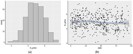
Figure 1.
Distribution of logarithms for unit prices (a) and trend of price change over time (b).
All observations assumed for analyses were grouped into two hierarchy levels. The first level refers to transactions and their attributes, while the second level concerns the location of the property in planning zones resulting from the division of the area into functional zones (Figure 2).
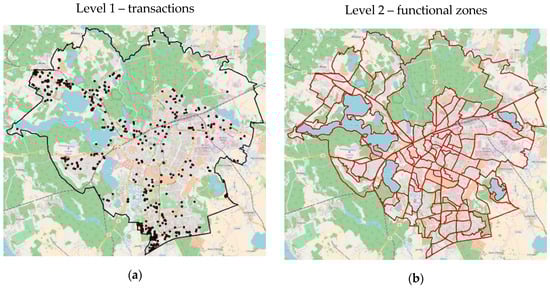
Figure 2.
Spatial location of transactions (a) and the layout of functional zones (b).
This division results, first of all, from planning documents (a study of conditions and directions for land development and a local zoning plan), as well as from natural conditions. The area in each distinguished zone is relatively uniform in terms of environment, the type of use and prevailing development. The administrative division was not used for the analysis due to the fact that, in this case, boundaries are imposed by formal considerations and not by market conditions. Therefore, an assumption was made that the adopted division into zones, which reflects location values, should also indicate areas that are relatively uniform in terms of prices and the factors affecting them. According to the assumptions made, this should result in a higher homogeneity of prices for properties situated in the same zone and at the same time, higher heterogeneity of properties situated in various zones.
4. Results and Discussion
This study was aimed not only at identification of spatial effects in the analysis of prices in the property market [56], but first of all at indicating the possibilities of applying the HSAR model to develop a land value map. Unquestionably, the use of the hierarchical data structure can contribute to improving the quality of obtained models [68]. The additional inclusion of spatial autocorrelation in the property market [31] makes it possible to construct a hierarchical spatial model, of not only a diagnostic [56], but also a predictive nature.
During the research period, apart from the HSAR model, three other models were constructed based on the same data set (LM: Linear Model, HLM: Hierarchical Linear Model, and SAR: Spatial Autoregressive Model), which made it possible to carry out a simple comparative analysis. Those models were then used to develop land value maps based on price prediction and residue analysis. The R environment with the packages HSAR, lme4, sp, spdep (among others) was used for statistical computing.
A classical multiple regression model (LM) provided a point of reference for further research and allowed a simple analysis of relations between assumed variables and the transaction price. Another model (SAR) was built based on the spatial autocorrelation phenomena. Detailed principles concerning the construction and testing of spatial autoregressive models are provided, among others, by [35] and [52]. A key issue can be, in this case, proper determination of the spatial weight matrix, reflecting mutual relations between objects located in space. During the studies, an assumption was made that mutual interaction between events in the property market (land prices) exponentially decreases along with the distance [56], while the range of similarity estimated on the basis of the variogram was about 2500 m. The estimated range confirms the results of previous analyses, e.g., References [69,70]. However, the threshold distance should also result from the spatial location of the transaction, and its values must be selected in such a way so as to ensure that each object is spatially related to other objects through the weight matrix. Therefore, the weight matrix was determined as [56]:
where d is the threshold value established based on data at 2,500 m. This matrix was then standardized with rows. Based on the Lagrange multiplier test [35], it was established that the proper model in this case would be the spatial lag model. In a subsequent model (HLM), fixed effects related to explained variables and random effects for the second hierarchy level were taken into account [71], without taking into consideration spatial dependencies. The identifier of property location in a given zone played the role of the second level hierarchy variable. The HSAR model assumes that the spatial weight matrix for the first level is the same as in the SAR model, while the weight matrix for the second level is based on the common threshold criterion (contiguity) of distinguished zones. The problem in this case was the emergence of islands, which means that some of the distinguished zones do not have any neighbour and therefore, a zero row occurs in the weight matrix. However, it means that the random effects for those zones in the HLM and HSAR model will be the same. The results of parameter estimation for individual models are presented in Table 3 and Table 4.
Table 3.
Results of estimation for LM and HLM models.
Table 4.
Results of estimation for SAR and HSAR models.
In the LM model, apart from the constant, six variables were proven to be statistically significant at a significance level of p < 0.05. The most significant variables were property right, distance from public transport stops and utilities network. Statistically insignificant variables included, among others, plot area and transaction date. The HLM model indicates four statistically significant variables. A comparison of both models indicates a slightly better fit of the HLM model. This is indicated by, among others, AIC. The residual standard deviation SEresid also proves the fact that the hierarchical model slightly better explains the price variability. In the SAR model, four variables proved statistically significant (property right, density of main roads, distance from public transport stops and utility network).
The coefficient of spatial autocorrelation ρ amounted to 0.551, which justifies application of a model using the spatial relations. In the HSAR model, six variables, as well as the constant for the model, is significant at the significance level of p < 0.05. Relatively high value AIC in HSAR model results from the effective number of parameters, which strongly depends on the variance of the group-level parameters [71]. In addition, a different method (Bayesian approach) was used to estimate the HSAR model, which may hinder the unambiguous interpretation of the common information criterion for all analysed models [64]. Therefore, when assessing the models, the criterion of minimizing errors was directed first of all. The value of the residual standard deviation was 0.361, which means that the average relative fit error is about 6.6% of the average transaction price logarithm. The value of spatial autocorrelation coefficient ρ is lower than in the SAR model, while autocorrelation specified for the second level in the hierarchy was 0.383, which proves moderate spatial dependency. The distribution of random effects for individual zones for the HLM and HSAR models is presented in Figure 3 and Figure 4. The distribution of random effects for both hierarchical models is very similar, which results from moderate spatial autocorrelation of prices at the level of zones. While those effects differ insignificantly, after converting logarithms into prices, it turns out that they can have a quite significant effect on the final land value map.
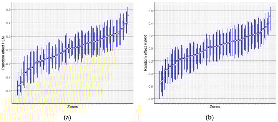
Figure 3.
Diagnostics of random elements of HLM (a) and HSAR (b) models (the chart presents random effects for individual zones, in the ascending order, specifying the confidence intervals for those effects).
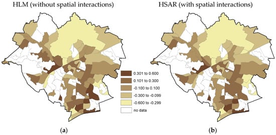
Figure 4.
Random effects for the second level (zone) for HLM (a) and HSAR (b) models.
Land value maps were generated by overlaying subsequent raster layers resulting from model coefficients, interpolated component ρWy (for SAR and HSAR models), random effects (for HLM and HSAR models) and the layer constructed based on the interpolation of residuals according to the scheme presented in Figure 5.
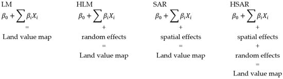
Figure 5.
Principles of overlaying layers while creating land value maps based on specific models.
Determination of a referential layer consisted in generating a raster, whose value corresponded to the model values created as a result of the sum of properly multiplied layers of explaining variables. It should be observed that seven variables among those assumed for the analyses can be referred to each point in the area under analysis. The beginning of 2018 was assumed as a date of study, ownership was assumed as the type of property rights and the assumed area was 1000 m2. In order to obtain the map of values, after overlaying individual layers, the obtained values in the form of logarithms were converted directly into the value in PLN. The value estimated on the basis of the LM model results from simple prediction, while the map generated on the basis of the SAR model required additional interpolation of the spatial lag (ρWy). Value maps developed on the basis of LM and SAR models are schematically presented in Figure 6.
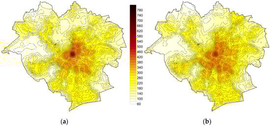
Figure 6.
Land value maps developed on the basis of LM (a) and SAR (b) models.
The distribution of values in both models is similar. Relatively high values prevail in the centre, decreasing when moving towards the city boundaries. Due to the fact that the developed maps are only of a demonstrative nature, water and forest areas were not excluded, although they should not be subject to the analysis.
For the HLM and HSAR models, random effects for zones also have to be taken into account. Therefore, the prediction of values was carried out as the first step, based on the fixed effects of the model and the mean value was then estimated for each of the zones, taking into account random effects. For the zones with no transactions, a zero value of random effect was assumed in the HLM model, while in the HSAR model, this value was obtained through interpolation. The obtained maps are schematically presented in Figure 7 and Figure 8.
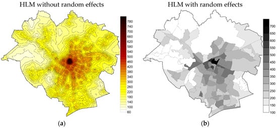
Figure 7.
Maps of land values developed based on HLM, (a) without random effect, and (b) with random effect.
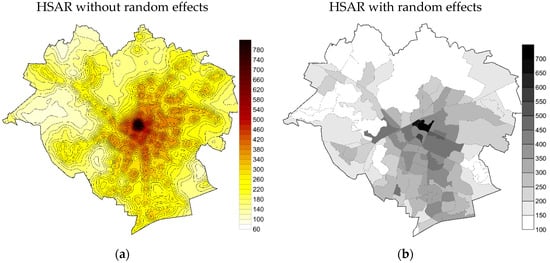
Figure 8.
Maps of land values developed based on HSAR, (a) without random effect, and (b) with random effect.
Differences in the estimation of land value obtained based on HLM and HSAR models are small and result from the assumption made with reference to spatial autocorrelation both at the first level (transactions) and the second level (zones). The similarity results first of all from the assumptions made concerning the effect of assumed factors on transaction prices.
The use of hierarchical spatial models can be an alternative or addition to the previously used methods for the development of land value maps. Geostatistics methods are commonly used in the development of such maps, which usually give satisfactory results [72,73]. However, it should be emphasized that hierarchical models can be particularly useful especially when we want to take into account the spatial hierarchy (e.g., division into districts or functional zones), which assumes rapid changes in value in space. Similar conclusions are drawn by, among others, Arribas et al. [68] used hierarchical models for price analysis in Alicante and Dong and Harris [42] who conducted research in Beijing.
5. Conclusions
The effect of value-forming factors on property prices can be modelled both with the use of classic regression models, as well as with models taking into account the spatial heterogeneity of prices and the hierarchical structure of market data. The study demonstrated that hierarchical models (HLM and HSAR) show a better fit to data than models not taking into account spatial hierarchy. This is proved, among others, by the value of the residual standard deviation. In the HSAR model, additionally taking spatial autocorrelation into account, a slightly lower level of SEresid errors was also found compared to the HLM model. Hierarchical spatial models, HSAR, take into account both micro-scale spatial effects and the context resulting from the location of specific observations at subsequent levels in the spatial hierarchy. Therefore, they carry greater informational content compared to classic models.
A significant effect of the research presented is the demonstration that HSAR models can be both diagnostic (identification of spatial effects) and predictive models (development of land value maps). Maps created with application of the HSAR model assume the constant nature of changes in land value inside the zone and discrete changes at the zone boundary. This corresponds to the actual situation, in which the urban space develops at the same time under the influence of strong planning intervention and the market demand for land, as determined by environmental values.
While the tradition of multilayer modelling has a long history, the role of this class of models still seems underestimated in spatial econometrics [70]. The studies conducted demonstrate that such models can be broadly applied in spatial management, in those places where phenomena of an economic nature are explicitly attributed to a specific location in space.
Author Contributions
Conceptualization, Radosław Cellmer and Katarzyna Kobylińska; Data preparation, Mirosław Bełej; Formal analysis, Radosław Cellmer and Katarzyna Kobylińska; Investigation, Mirosław Bełej; Methodology, Radosław Cellmer and Katarzyna Kobylińska; Visualization, Radosław Cellmer.
Funding
This research received no external funding.
Conflicts of Interest
The authors declare no conflict of interest.
Abbreviations
The following abbreviations are used in this manuscript:
| HLM | Hierarchical Linear Model |
| HSAR | Hierarchical Spatial Autoregressive |
| LM | Linear Model |
| SAR | Spatial Autoregressive |
Appendix A
Histograms and qq-plots of all investigated variables
| lnprice | 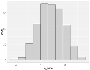 | 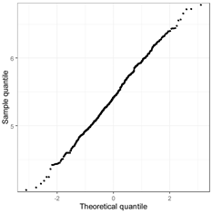 |
| date | 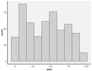 | 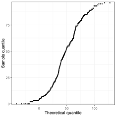 |
| right | 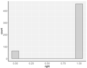 | 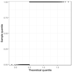 |
| lnarea | 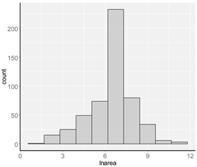 | 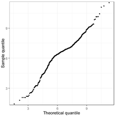 |
| type | 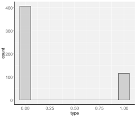 | 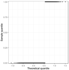 |
| lnlake | 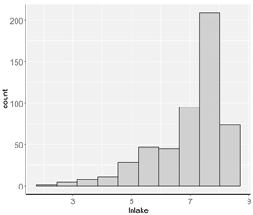 | 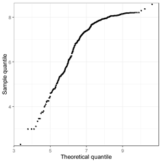 |
| lnforest |  | 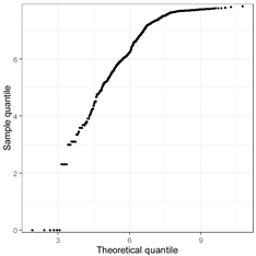 |
| densdev | 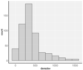 | 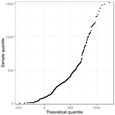 |
| densroad | 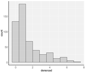 | 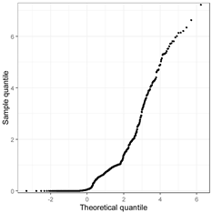 |
| lncentr | 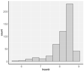 | 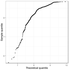 |
| lnbus | 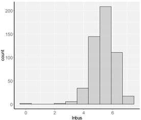 | 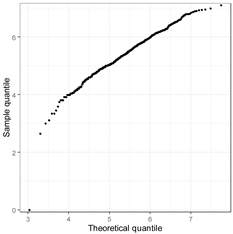 |
| utility | 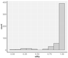 | 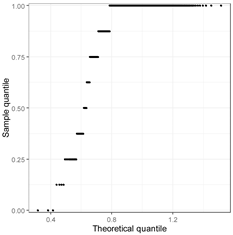 |
References
- Fujita, M.; Thisse, J.F. Economics of Agglomeration: Cities, Industrial Location, and Globalization; Cambridge University Press: Cambridge, UK, 2013. [Google Scholar]
- Sassen, S. Cities in a World Economy; Sage Publications: Thousand Oaks, CA, USA, 2018. [Google Scholar]
- Le Galès, P. European Cities: Social Conflicts and Governance; Oxford University Press: Oxford, UK, 2002. [Google Scholar]
- Hamnett, C. Social polarisation in global cities: Theory and evidence. Urban Stud. 1994, 31, 401–424. [Google Scholar] [CrossRef]
- Henderson, V.; Kuncoro, A.; Turner, M. Industrial development in cities. J. Political Econ. 1995, 103, 1067–1090. [Google Scholar] [CrossRef]
- Semanjski, I.; Gautama, S. Smart city mobility application—Gradient boosting trees for mobility prediction and analysis based on crowdsourced data. Sensors 2015, 15, 15974–15987. [Google Scholar] [CrossRef] [PubMed]
- García-Hernández, M.; de la Calle-Vaquero, M.; Yubero, C. Cultural heritage and urban tourism: Historic city centres under pressure. Sustainability 2017, 9, 1346. [Google Scholar] [CrossRef]
- Przybyła, K.; Kachniarz, M.; Hełdak, M. The Impact of Administrative Reform on Labour Market Transformations in Large Polish Cities. Sustainability 2018, 10, 2860. [Google Scholar] [CrossRef]
- Renigier-Biłozor, M.; Biłozor, A.; Wisniewski, R. Rating engineering of real estate markets as the condition of urban areas assessment. Land Use Policy 2017, 61, 511–525. [Google Scholar] [CrossRef]
- Brzezicka, J.; Wisniewski, R.; Figurska, M. Disequilibrium in the real estate market: Evidence from Poland. Land Use Policy 2018, 78, 515–531. [Google Scholar] [CrossRef]
- Colwell, P.F.; Munneke, H.J. Estimating a Price Surface for Vacant Land in an Urban Area. Land Econ. 2003, 79, 15–28. [Google Scholar] [CrossRef]
- Earnhart, D. Using Contingent-Pricing Analysis to Value Open Space and Its Duration at Residential Locations. Land Econ. 2006, 82, 17–35. [Google Scholar] [CrossRef]
- Haughwout, A.; Orr, J.; Bedoll, D. The Price of Land in the New York Metropolitan Area. Curr. Issues Econ. Financ. 2008, 14, 1–7. [Google Scholar]
- Bryan, K.A.; Sarte, P.G. Semiparametric Estimation of Land Price Gradients Using Large Data Sets. Fed. Reserve Bank Richmond Econ. Q. 2009, 95, 53–74. [Google Scholar]
- Źróbek, S.; Grzesik, K. Modern Challenges Facing the Valuation Profession and Allied University Education in Poland. Real Estate Manag. Val. 2013, 21, 14–18. [Google Scholar] [CrossRef]
- Wójciak, E. The Essence of Equivalent Markets in Determining the Market Value of Land Property for Variable Planning Factors. Real Estate Manag. Val. 2016, 24, 71–82. [Google Scholar] [CrossRef]
- Munroe, D.K. Exploring the Determinants of Spatial Pattern in Residential Land Markets: Amenities and Disamenities in Charlotte. Environ. Plan. B Plan. Des. 2007, 34, 336–354. [Google Scholar] [CrossRef]
- Ogryzek, M.; Wisniewski, R.; Kauko, T. On Spatial Management Practices: Revisiting the “Optimal” Use of Urban Land. Real Estate Manag. Val. 2018, 26, 24–34. [Google Scholar] [CrossRef]
- Liu, Y.; Zheng, B.; Huang, L.; Tang, X. Urban Residential Land Value Analysis: Case Danyang. Geo. Spat. Inf. Sci. 2007, 10, 228–234. [Google Scholar] [CrossRef]
- Bugs, G. Urban Land Value Map: A Case Study in Eldorado do Sul—Brazil, Erasmus Mundus Master of Science on Geospatial Technologies, Instituto Superior de Estatística e Gestão da Informação; Universidade Nova de Lisboa: Lisbon, Portugal, 2007. [Google Scholar]
- Benjamin, J.D.; Randall, S.; Guttery, R.S.; Sirmans, C.F. Mass Appraisal: An Introduction to Multiple Regression Analysis for Real Estate Valuation. J. Real Estate Pract. Educ. 2004, 7, 65–77. [Google Scholar]
- Noelwah, R.N. The Effect of Environmental Zoning and Amenities on Property Values: Portland, Oregon. Land Econ. 2005, 81, 227–246. [Google Scholar]
- Cotteleer, G.; Gardebroek, C.; Luijt, J. Market Power in a GIS-Based Hedonic Price Model of Local Farmland Markets. Land Econ. 2008, 84, 573–592. [Google Scholar] [CrossRef]
- Hannoen, M. Predicting urban land prices: A comparison of four approaches. Int. J. Strateg. Prop. Manag. 2008, 12, 217–236. [Google Scholar] [CrossRef]
- Páez, A. Recent research in spatial real estate hedonic analysis. J. Geogr. Syst. 2009, 11, 311–316. [Google Scholar] [CrossRef]
- Montero, J.M.; Larraz, B. Estimating Housing Prices: A Proposal with Spatially Correlated Data. Int. Adv. Econ. Res. 2010, 16, 39–51. [Google Scholar] [CrossRef]
- Ludiema, G.; Makokha, G.; Ngigi, M.M. Development of a Web-Based Geographic Information System for Mass Land Valuation: A Case Study of Westlands Constituency, Nairobi County. J. Geogr. Inf. Syst. 2018, 10, 283–300. [Google Scholar] [CrossRef]
- Fik, T.J.; Ling, D.C.; Mulligan, G.F. Modeling Spatial Variation in Housing Prices: A Variable Interaction Approach. Real Estate Econ. 2003, 31, 623–646. [Google Scholar] [CrossRef]
- Bourassa, S.C.; Cantoni, E.; Hoesli, M. Predicting House Prices with Spatial Dependence: A Comparison of Alternative Methods. J. Real Estate Res. 2010, 32, 139–160. [Google Scholar]
- Anselin, L. GIS Research Infrastructure for Spatial Analysis of Real Estate Markets. J. Hous. Res. 1998, 9, 113–133. [Google Scholar]
- Basu, S.; Thibodeau, T. Analysis of spatial autocorrelation in house prices. J. Real Estate Financ. 1998, 17, 61–85. [Google Scholar] [CrossRef]
- Tu, Y.; Sun, H.; Yu, S. Spatial autocorrelations and urban housing market segmentation. J. Real Estate Financ. Econ. 2007, 34, 385–406. [Google Scholar] [CrossRef]
- Bowen, W.M.; Mikelbank, B.A.; Prestegaard, D.M. Theoretical and Empirical Considerations Regarding Space in Hedonic Housing Price Model Applications. Growth Chang. 2001, 32, 466–490. [Google Scholar] [CrossRef]
- LeSage, J. Introduction to Spatial Econometrics; De Boeck Supérieur: Paris, France, 2010; pp. 19–44. [Google Scholar] [CrossRef]
- Anselin, L. Spatial Econometrics; Bruton Center School of Social Sciences; University of Texas at Dallas: Richardson, TX, USA, 1999. [Google Scholar]
- Longford, N.T. Random Coefficient Models. In Handbook of Statistical Modeling for the Social and Behavioral Sciences; Arminger, G., Clogg, C.C., Sobel, M.E., Eds.; Springer: Boston, MA, USA, 1993; pp. 519–570. [Google Scholar]
- Fotheringham, A.S.; Brunsdon, C.; Charlton, M.E. Geographically Weighted Regression: The Analysis of Spatially Varying Relationships; John Wiley & Sons: Hoboken, NJ, USA, 2003. [Google Scholar]
- Demetriou, D. The assessment of land valuation in land consolidation schemes: The need for a new land valuation framework. Land Use Policy 2016, 54, 487–498. [Google Scholar] [CrossRef]
- Corrado, L.; Fingleton, B. Where is the economics in spatial econometrics? J. Reg. Sci. 2012, 52, 210–239. [Google Scholar] [CrossRef]
- Baltagi, B.H.; Fingleton, B.; Pirotte, A. Spatial lag models with nested random effects: An instrumental variable procedure with an application to English house prices. J. Urban Econ. 2014, 80, 76–86. [Google Scholar] [CrossRef]
- Łaszkiewicz, E. Multiparametric and hierarchical spatialautoregressive models: The evaluation of the misspecification of spatial effects using a monte carlo simulation. Acta Univ. Lodz. Folia Oecon. 2014, 5, 63–75. [Google Scholar]
- Dong, G.; Harris, R.; Jones, K.; Yu, J. Multilevel Modelling with Spatial Interaction Effects with Application to an Emerging Land Market in Beijing. PLoS ONE 2015, 10, 1–18. [Google Scholar] [CrossRef]
- Liu, B.; Mavrin, B.; Niu, D.; Kong, L. House Price Modeling over Heterogeneous Regions with Hierarchical Spatial Functional Analysis. In Proceedings of the IEEE 16th International Conference on Data Mining (ICDM), Barcelona, Spain, 12–15 December 2016. [Google Scholar] [CrossRef]
- Moreira de Aguiar, M.; Simões, R.; Braz Golgher, A. Housing market analysis using a hierarchical–spatial approach: The case of Belo Horizonte, Minas Gerais. Braz. Reg. Stud. Reg. Sci. 2014, 1, 116–137. [Google Scholar] [CrossRef]
- Kulesza, S.; Bełej, M. Local Real Estate Markets in Poland as a Network of Damped Harmonic Oscillators. Acta Phys. Pol. A 2015, 127, 99–102. [Google Scholar] [CrossRef]
- Krause, A.L.; Bitter, C. Spatial econometrics, land values and sustainability: Trends in real estate valuation research. Cities 2012, 29, 19–25. [Google Scholar] [CrossRef]
- Osland, L. An application of spatial econometrics in relation to hedonic house price modeling. J. Real Estate Res. 2010, 32, 289–320. [Google Scholar]
- Bhat, C.R. A heteroscedastic extreme value model of intercity travel mode choice. Transp. Res. Part B Methodol. 1995, 29, 471–483. [Google Scholar] [CrossRef]
- Greene, W.H.; Hensher, D.A. Heteroscedastic control for random coefficients and error components in mixed logit. Transp. Res. Part E Logist. Transp. Rev. 2007, 43, 610–623. [Google Scholar] [CrossRef]
- Wilhelmsson, M. Spatial Model in Real Estate Economics. Hous. Theory Soc. 2002, 19, 92–101. [Google Scholar] [CrossRef]
- Páez, A.; Scott, D.M. Spatial statistics for urban analysis: A review of techniques with examples. GeoJournal 2004, 61, 53–67. [Google Scholar] [CrossRef]
- Arbia, G. Spatial Econometrics: Statistical Foundations and Applications to Regional Convergence; Springer: Berlin, Germany, 2006. [Google Scholar]
- Vega, S.H.; Elhorst, J.P. The SLX Models. J. Reg. Sci. 2015, 55, 339–363. [Google Scholar] [CrossRef]
- Fotheringham, A.S.; O’Kelly, M.E. Spatial Interaction Models: Formulations and Applications; Kluwer Academic Pub: Dordrecht, The Netherlands, 1989. [Google Scholar]
- Diggle, P.; Heagerty, P.; Liang, K.Y.; Zeger, S. Analysis of Longitudinal Data; Oxford University Press: Oxford, UK, 2002. [Google Scholar]
- Dong, G.; Harris, R. Spatial Autoregressive Models for Geographically Hierarchical Data Structures. Geogr. Anal. 2015, 47, 173–191. [Google Scholar] [CrossRef]
- Bivand, R.; Sha, Z.; Osland, L.; Thorsen, I.S. A comparison of estimation methods for multilevel models of spatially structured data. Spat. Stat. 2017, 21, 440–459. [Google Scholar] [CrossRef]
- Goldstein, H. Multilevel Statistical Models; John Wiley & Sons: Hoboken, NJ, USA, 2011. [Google Scholar]
- Jones, K. Specifying and Estimating Multi-Level Models for Geographical Research. Trans. Inst. Br. Geogr. 1991, 16, 148–159. [Google Scholar] [CrossRef]
- Osland, L.; Thorsen, I.S.; Thorsen, I. Accounting for local spatial heterogeneities in housing market studies. J. Reg. Sci. 2016, 56, 895–920. [Google Scholar] [CrossRef]
- Chasco, C.; Le Gallo, J. Hierarchy and spatial autocorrelation effects in hedonic models. Econ. Bull. 2012, 32, 1474–1480. [Google Scholar]
- Brunauer, W.; Lang, S.; Umlauf, N. Modelling house prices using multilevel structured additive regression. Stat. Model. 2013, 13, 95–123. [Google Scholar] [CrossRef]
- Łaszkiewicz, E.; Dong, G.; Harris, R.J. The Effect Of Omitted Spatial Effects And Social Dependence In The Modelling Of Household Expenditure For Fruits And Vegetables. Comp. Econ. Res. 2014, 17, 155–172. [Google Scholar] [CrossRef]
- Gelman, A.; Carlin, J.B.; Stern, H.S.; Rubin, D.B. Bayesian Data Analysis, 2nd ed.; Chapman & Hall/CRC: London, UK, 2003. [Google Scholar]
- D’Amato, M. Comparing rough set theory with multiple regression analysis as automated valuation methodologies. Int. Real Estate Rev. 2007, 10, 42–65. [Google Scholar]
- García, N.; Gámes, M.; Alfaro, E. ANN + GIS: An automated system for property valuation. Neurocomputing 2008, 71, 733–742. [Google Scholar] [CrossRef]
- Kontrimas, V.; Verikas, A. The mass appraisal of real estate by computational intelligence. Appl. Soft Comput. 2011, 11, 443–448. [Google Scholar] [CrossRef]
- Arribas, J.; García, F.; Guijarro, F.; Oliver, J.; Tamošiūnienė, R. Mass Appraisal of Residential Real Estate Using Multilevel Modelling. Int. J. Strateg. Prop. Manag. 2016, 20, 77–87. [Google Scholar] [CrossRef]
- Gelfand, A.E.; Zhu, L.; Carlin, B.P. On the Change of Support Problem for Spatiotemporal Data. Biostatistics 2001, 2, 31–45. [Google Scholar] [CrossRef]
- Banerjee, S.; Carlin, B.P.; Gelfand, A.E. Hierarchical Modeling and Analysis for Spatial Data; CRC Press/Chapman & Hall. Monographs on Statistics and Applied Probability: Boca Raton, FL, USA, 2014; p. 562. [Google Scholar]
- Gelman, A.; Hwang, J.; Vehtari, A. Understanding predictive information criteria for Bayesian models. Stat Comput. 2014, 24, 997–1016. [Google Scholar] [CrossRef]
- Luo, J.; Wei, Y.D. A Geostatistical Modeling of Urban Land Values in Milwaukee, Wisconsin. Geogr Inf Sc. 2004, 10, 49–57. [Google Scholar] [CrossRef]
- Cellmer, R.; Źróbek, S. The Cokriging Method in the Process of Developing Land Value Maps. In Proceedings of the 2017 Baltic Geodetic Congress (BGC Geomatics), Gdansk, Poland, 22–25 June 2017. [Google Scholar] [CrossRef]
© 2019 by the authors. Licensee MDPI, Basel, Switzerland. This article is an open access article distributed under the terms and conditions of the Creative Commons Attribution (CC BY) license (http://creativecommons.org/licenses/by/4.0/).