Comprehensive Analysis of System Calibration between Optical Camera and Range Finder

Abstract

This paper describes the comprehensive analysis of system calibration between an optical camera and a range finder. The results suggest guidelines for accurate and efficient system calibration enabling high-quality data fusion. First, self-calibration procedures were carried out using a testbed designed for both the optical camera and range finder. The interior orientation parameters of the utilized sensors were precisely computed. Afterwards, 92 system calibration experiments were carried out according to different approaches and data configurations. For comparison of the various experimental results, two measures, namely the matching rate of fusion data and the standard deviation of relative orientation parameters derived after system calibration procedures, were considered. Among the 92 experimental cases, the best result (the matching rate of 99.08%) was shown for the use of the one-step system calibration method and six datasets from multiple columns. Also, the root mean square values of the residuals after the self- and system calibrations were less than 0.8 and 0.6 pixels, respectively. In an overall evaluation, it was confirmed that the one-step system calibration method using four or more datasets provided more stable and accurate relative orientation parameters and data fusion results than the other cases.

1. Introduction

In recent years, 3D modeling has been applied in various areas including public safety, virtual environments, fire and police planning, location-based services, environmental monitoring, intelligent transportation, structural health monitoring, underground construction, motion capturing, and so on [1]. In general, 3D modeling usually can be constructed through several procedures after acquiring the data from a sensor system. The systems for 3D modeling are largely divided into single-modal and multi-modal types. The single-modal system consists of one type of sensor: in most cases, multiple optical cameras. By contrast, the multi-modal system comprises at least two types of sensors, such as laser scanning sensors, optical cameras, and range finders [2]. More specifically, the single-modal system can be built at relatively low cost and has the advantage of data production with high-resolution RGB-D data (color and depth). As a disadvantage, however, when area images of areas with low levels of information on feature points or with repetitive similar textures are considered, the accuracy of the 3D model of the area is markedly lowered.

On the other hand, the multi-modal system generally consists of optical cameras providing color information and other sensors giving depth information, such as light detection and ranging (LiDAR), laser line scanners, and range finders [3]. The system has the advantage of the fact that the shapes of objects are reconstructed more accurately [3]. Also, the quality of data in areas lacking texture or with discontinuous depths is higher than in the single-modal system [4].

Because of the benefits of using the multi-modal system, various types of data acquisition systems with different sensors have recently been developed [3]. The sensor system comprised of optical cameras and range finders is one of the well-known multi-modal systems. An intensity image from the range finder can also be provided in the form of a 2D matrix, similar to an optical camera, and each image pixel has a depth value. Also, as range finders are relatively lower-priced than laser line scanners and LiDAR, the sensor system can be configured at lower cost.

On the other hand, the optical-range-finder system also has disadvantages attributable to the characteristics of range finders. In general, range finders have lower resolutions than LiDAR. Additionally, they enable obtainment of data only within short distances, and thus, when the distance to an object becomes longer than a certain threshold, the quality of 3D models will deteriorate. Moreover, since range finders measure depth information using infrared rays, they produce high levels of noise when encountering natural light (e.g., strong sunlight). In cases of data acquisition in indoor environments, the disadvantages of using the optical-range-finder system can be significantly reduced, since the distance to indoor objects or structures is sufficiently short, and the influences of sunlight are minimized.

In this context, this paper will discuss a multi-modal system comprised of an optical camera and a range finder to be utilized in indoor environments. This research will also focus on an analysis of the factors affecting the quality of fusion data (i.e., RGB-D data) and will provide guidelines for obtaining accurate fusion results.

The remainder of this paper is organized as follows. Section 2 reviews the latest research in self- and system calibrations that are essential for data fusion using a multi-modal system. Section 3 describes the sensor geometric functional models and testbed utilized for the present calibrations. Section 4 outlines the procedures of the calibration and evaluation strategy in detail. Section 5 presents the experimental results and a related discussion. Finally, Section 6 draws conclusions on the findings of this research and looks ahead to upcoming work.

2. Related Work

Self-calibration of each sensor as well as system calibration should be carried out as prerequisite procedures to merge different types of datasets acquired from different sensors. This will enable compilation of an accurate RGB-D dataset using the multi-modal system. Thus, in this section, the recent work on self-calibration and system calibration is presented and discussed.

More specifically, self-calibration is a procedure to determine the interior orientation parameters (IOPs: principal point coordinates, focal length, and distortion parameters) that express the characteristics of each sensor. The images of optical cameras include radial, and decentering lens distortions. And, the depth data of range finders include various noises such as signal-dependent shot noise, systematic bias, and random noise [5].

System calibration, on the other hand, determines the geometric relationship between the sensors employed in the data acquisition system. The geometric relationship usually can be expressed in the form of relative orientation parameters (ROPs) including 3 translation and 3 rotation parameters.

In this context, data fusion can be performed more accurately when self-calibration for each sensor is precisely rendered. In almost all cases, self-calibration is a prerequisite for system calibration.

In the case of self-calibration of optical cameras, the methods and accuracies have been sufficiently verified and well-established [6,7,8,9]. Meanwhile, various studies have been conducted on the self-calibration of range finders. In these studies, various self-calibration methods have been proposed and compared [10,11]. Lichti et al. [10] suggested a method of simultaneous adjustment of image points and range observations in range finders (SR3000 & SR4000). Lichti and Kim [11] conducted self-calibration of range finders using three different methods (i.e., one-step integrated, two-step independent, and two-step dependent methods), and performed a comparative evaluation of those approaches. Their results showed that using the one-step integrated method resulted in the highest accuracy. Lichti and Qi [12] improved the accuracy of self-calibration using depth information and measured distances between targets on a testbed. Jamtsho [13] derived distortion models and determined parameters for range finders by applying the Akaike information criterion method to range-finder calibration procedures. Westfeld et al. [14] obtained IOPs, and range-value calibration constants by performing self-calibration on range finders using a sphere-shaped testbed. Lindner and Kolb [15] calibrated the IOPs of intensity images using a chessboard-style testbed, and calibrated the range values using B-spline curves. Some researchers have used a lookup table for calibration of depth values. Shim et al. [3] calibrated range-finder depth values using a lookup table, and derived lens distortion parameters for each sensor prior to system calibration between optical cameras and time-of-flight (TOF) sensors. Zhu et al. [16], using a chessboard-type testbed, produced a lookup table for the calibration of depth values for each pixel in the TOF sensor. In their review of the previous studies on self-calibration, the authors noted that various self-calibration approaches, especially those for optical cameras and TOF sensors, have been verified through comparative evaluations. Therefore, they adopted one of those existing methods for implementation as a prerequisite to system calibration in the present research.

The methods of system calibration in the existing studies can be broadly divided into one-step and two-step methods. In the case of the one-step method, the locations of remaining sensors are calculated based on a reference camera. The exterior orientation parameters (EOPs) of the reference camera and the ROPs of the other cameras are set as unknown, and both the EOPs and ROPs are calculated simultaneously by a single bundle adjustment. On the other hand, the two-step method first calculates the EOPs of each sensor through separate bundle adjustments and then sequentially determines the ROPs between the sensors.

Mikhelson et al. [17] conducted self-calibration on the Kinect sensor and an optical-range finder, and performed the one-step system calibration. Van den Bergh and Van Gool [18] performed self-calibration of optical camera and TOF sensor using Matlab camera calibration tool box and checker board. Also, one-step system calibration was involved in that study. Afterwards, they used the system calibration results for the application of hand gesture interaction. However, they did not consider the calibration of the range distortions. Hansard et al. [19] and Zhu et al. [16] developed a system comprised of two optical cameras and one range finder, attempted to merge 3D information produced using RGB stereo images with the depth data of range finders, and calculated the ROP information through one-step system calibration. Hansard et al. [19] did not involve the calibration of the range distortions in their study. On the other hand, Zhu et al. [16] used a lookup table to get rid of the range distortions. Herrera et al. [20] simultaneously calibrated two optical cameras, a depth camera, and ROPs between the sensors. Corner and plane information from a checkerboard is utilized for calibrating the optical cameras and a depth camera, respectively. Also, they performed the one-step system calibration in that study. Wu et al. [21] first performed self-calibration of CCD camera and TOF intensity image using Matlab calibration tool box. The self-calibration results were then used for one-step system calibration. Range distortions were not considered in their research. Jung et al. [22] performed precise self-and system calibration for accurate color and depth data fusion. They, first, obtained the IOPs and distortion parameters of each sensor and calibrated the distance of the range finder for each pixel using 2.5D pattern testbed. Afterwards, one-step system calibration was performed with calibrated data. Vidas et al. [23] conducted one-step system calibration on multi-modal sensor system (comprised of the Kinect sensor and a thermal-infrared camera) for building interior temperature mapping. Prior to the system calibration, self-calibration was carried out only for the thermal infrared camera; not for the Kinect sensor. Before the system calibration process, image distortions of the thermal camera were removed. And, 2D and 3D lines were extracted from the thermal-infrared image and Kinect range data respectively; and they were utilized for the next step, the system calibration.

Alternatively, Shim et al. [3] conducted two-step system calibration for data fusion between optical camera and TOF sensor. In that study, prior to the system calibration, lens distortion parameters of sensors and a look-up table for range data calibration were calculated. And relative pose between the involved sensors was calculated by using each sensor’s EOPs calculated from respective bundle adjustments (i.e., two-step system calibration). One also should know that focal length estimation for the involved sensors was not considered in their research. Lindner et al. [24] performed two-step system calibration with pre-calibrated CCD camera and TOF sensor data. Self-and system calibration were conducted using a checker board style testbed and OpenCV library. The self-calibration scopes of two sensors included principal point coordinates, focal length, and distortion parameters; but, not range data distortions. Dorit et al. [25] carried out the calibration procedures for the multi-modal system comprised of a 3D laser scanner, a thermal camera, and a color camera. They first conducted the self-calibration of the optical and thermal sensors; but not the 3D laser scanner. Their two-step system calibration produced several pairs of ROPs, and they selected the best one which minimizes the re-projection error for all image pairs. Mattero et al. [26] generated a multi-modal sensor system for people tracking, and the system is based on multi-camera network composed by three Kinect sensors and three SR4500 TOF cameras. They utilized OpenPTrack software in the calibration steps. Only focal length, principal point coordinates, and lens distortions were considered in the self-calibration procedures. Also, two-step system calibration was carried out in that research.

After reviewing the latest studies relevant to optical-range-finder systems, we found that in terms of system calibration, most studies have proposed their own calibration methods and evaluations without any explanation or analysis of data acquisition configurations. Also, in most studies, there was no comparative analysis of different system calibration (especially, one-step and two-step) approaches. One-step system calibration approaches deal with only one set of ROPs (i.e., 3 translations and 3 rotations) between two sensors in all workflows. When many sensors are involved; however, the sensor geometric models will be more complicated. On the other hand, two-step system calibration approaches have relatively simple geometric models and it is easy to implement the approaches because the EOPs of each sensor will be treated separately. However, the ROPs between the sensors will be determined through the post-processing work using all the estimated EOPs.

Moreover, we also found that most of the previous studies on system calibration also included self-calibration as a prerequisite in their approaches. However, some of the studies simply used nominal values of IOPs provided by the sensor manufacturer in their system calibration procedures, without any correction [17]. Also, other studies did not consider some IOPs such as range distortion parameters ([17,21,24,25,26]) and focal length ([3]) in their self-calibration procedures. To minimize the effect of the self-calibration quality on the accuracy of system calibration and also the quality of RGB-D data produced, the proposed study considers all the involved sensors and their IOPs. At this stage, one should note that the self-calibration approaches of the optical and TOF cameras are well-established. Hence, the proposed study will adopt the existing self-calibration approaches in order to deal with all relevant parameters and thereby guarantee acceptable self-calibration results.

In this light, in the present research, (1) comparative evaluations of the different system calibration methods (i.e., one-step and two-step approaches) and (2) an analysis of the effects of the data acquisition configuration (i.e., different geometrical locations and numbers of datasets) on the quality of the final products (i.e., ROPs or fusion data) were performed. Finally, guidelines for accurate and efficient system calibration and high-quality data fusion were derived.

3. Sensor Geometric Functional Models and Calibration Testbed

3.1. Testbed Designed for Calibration Procedure

In this study, a testbed for the calibration procedure was constructed in consideration of the relevant optical camera and range finder characteristics (Figure 1). The testbed’s chessboard configuration and white circular patterns are used as control points (CPs) for the optical camera and the range finder, respectively. The configuration of the circular pattern target is adopted from [10,11,12] and the number of targets are slightly reduced since we have enough number of targets shown on the acquired images at the different distances. The white circle and its calculated centroid are very useful for the range finder, but not for the optical camera. To resolve this problem, additional targets with chessboard pattern were installed on the testbed plane for the optical camera (Figure 1b,c). The testbed dimensions are 4 m (height) by 4.9 m (width). As can be seen in the figure, the chessboard targets were arranged in different depths from the surface of the white circular patterns.

Figure 1. Testbed: (a) front view; (b) side view; (c) chessboard pattern target.

3.2. Sensors and Mathematical Models

The optical-range-finder system used in the experiment was configured through the installation of a Canon 6D DSLR camera (optical sensor) and a SR4000 range finder on a single aluminum frame (Figure 2). Figure 2a,b show the side view and front view of the installed optical-range-finder system, respectively. The produced sensor system provides, for each round of filming, RGB image data from the optical camera along with intensity and range data from the range finder. More detailed specifications of the sensors are shown in Table 1.

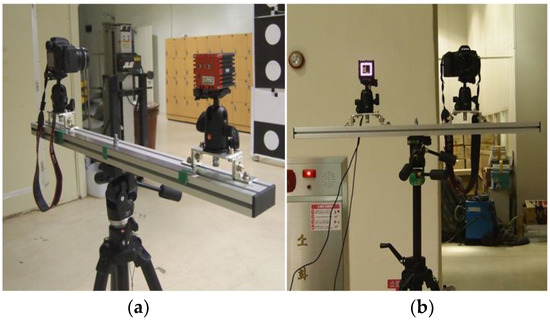
Figure 2. Installed optical-range-finder system: (a) side view; (b) front view.

Table 1. Specifications of sensors.

Sensor Type	Model Name	Image Size (Pixels)	Pixel Size (mm)	Focal Length (Nominal/mm)	Field of View
Optical camera	Canon 6D	5472 × 3648	0.00655	35	63°
Range finder	SR4000 (Mesa imaging)	176 × 144	0.04	5.8	69° (h) × 56° (v)

The imaging geometry for the RGB image data (acquired from the optical camera) and the intensity data (acquired from the range finder) are expressed in functional models based on the collinearity condition, as seen in Equations (1)–(3) ([27]). The range data (acquired from the range finder) are expressed in the Euclidean distance model, as seen in Equation (4).

$$x=x_p-f\frac{m11\left(X-X0\right)+m12\left(Y-Y0\right)+m13\left(Z-Z0\right)}{m31\left(X-X0\right)+m32\left(Y-Y0\right)+m33\left(Z-Z0\right)}+\Delta x$$

(1)

$$y=y_p-f\frac{m21\left(X-X0\right)+m22\left(Y-Y0\right)+m23\left(Z-Z0\right)}{m31\left(X-X0\right)+m32\left(Y-Y0\right)+m33\left(Z-Z0\right)}+\Delta y$$

(2)

$$Rotation matrix M\left(\omega ,\phi ,\kappa \right)=\left[\begin{array}{ccc}m11& m12& m13\\ m21& m22& m23\\ m31& m32& m33\end{array}\right]$$

(3)

$$\rho =\sqrt{{\left(X-X0\right)}^2+{\left(Y-Y0\right)}^2+{\left(Z-Z0\right)}^2}+\Delta \rho$$

(4)

In the equations, x and y are the image coordinates of the sensor data. ∆x and ∆y are the distortions of the image coordinates. x_p and y_p are the image coordinates of the principal point and f is the focal length. m₁₁ to m₃₃ are the components of the rotation matrix M. ω is the primary rotation along X-axis, $\phi$ is the secondary rotation along Y-axis, and κ is the tertiary rotation along Z-axis. X, Y, and Z are the ground coordinates of the control point. X0, Y0, and Z0 are three of the exterior orientation parameters of the sensor (sensor position). ρ is the measured range value, and ∆ρ is the distortion of the range value.

Standard lens distortion models, as seen in Equations (5)–(7), are utilized for the optical camera and range finder (refer to [6,7,8]). Also, the systematic range bias (∆ρ) model for the range finder is seen in Equations (8) (refer to [10,11,12]).

$$\Delta x=\overline{x}\left(K_1{r}^2+K_2{r}^4+K_3{r}^6\right)+P_1\left(r^2+2{\overline{\mathrm{x}}}^2\right)+2P_2\overline{x}\overline{y}+A_1\overline{x}+A_2\overline{y}$$

(5)

$$\Delta y=\overline{y}\left(K_1{r}^2+K_2{r}^4+K_3{r}^6\right)+2P_1\overline{x}\overline{y}+P_2\left(r^2+2{\overline{y}}^2\right)$$

(6)

$$\overline{x}=x-x_p,\overline{y}=y-y_p,\mathrm{r}=\sqrt{{\overline{x}}^2+{\overline{y}}^2}$$

(7)

$$\Delta \rho =d_0+d_1\rho +{\displaystyle \sum }_{k=1}^3\left[d_{2k}\sin \frac{2^k\pi }{U}\rho \right]+e_1\overline{x}+e_2\overline{y}+e_{3}r+e_r{r}^2+{\displaystyle \sum }_{m=2}^3{\displaystyle \sum }_{n=0}^m{e}_{3m+n-1}{\overline{x}}^{m-n}{\overline{y}}^n$$

(8)

In the equations, K₁, K₂, and K₃ are radial lens distortion parameters, P₁ and P₂ are the decentering lens distortion parameters, A₁ and A₂ are the electronic biases (affinity and shear), d₀ is the rangefinder offset, d₁ is the scale error, and d₂ to d₇ are the cyclic errors; U is the unit wavelength, e₁ and e₂ are clock skew errors, and e₃ to e₁₁ are empirical errors.

4. Calibrations and Comparative Evaluation Strategy

The experiments were conducted, as seen in Figure 3, in four phases: data acquisition, self-calibration, system calibration, and data fusion. First, in the data acquisition phase, optical and range-finder data were acquired for use in self-calibration and system calibration, respectively. The IOPs for the individual sensors were calculated through the self-calibration procedure. Afterwards, the estimated parameters were utilized for the system calibration procedure. The system calibration was performed by the one-step and two-step approaches. Finally, the fusion of optical and range-finder data was performed using ROPs calculated through the system calibration procedure. More detailed explanations of the approach are provided in the following sub-sections.

Figure 3. Calibration procedures proposed.

4.1. Self-Calibration

Since the self-calibration approaches for the individual sensors have been thoroughly reviewed and evaluated in existing studies, the present study carried out the self-calibration based on existing methods. The self-calibration of the optical sensor was first performed using the commonly used least square estimation method - bundle block adjustment [6,7,8,9]. The self-calibration of the range finder was also performed based on the one-step integrated method, which was found to be more accurate than other methods in a comparative evaluation [11].

The datasets for the self-calibration procedures were acquired using the optical-range-finder system (shown in Figure 2). They included optical camera images, range-finder intensity images, and range data for all pixels in the intensity images. Fifteen datasets were acquired for the self-calibration procedures; among them, three were obtained after vertically erecting the system to minimize the correlation between the IOPs and EOPs of the individual sensors. The locations of the data acquired for the self-calibration procedures are shown in Figure 4. The datasets were acquired at the center, left and right sides of the testbed in order to keep the images converged. After carrying out the self-calibration procedures to estimate the IOPs, the values were utilized in the system calibration procedures.

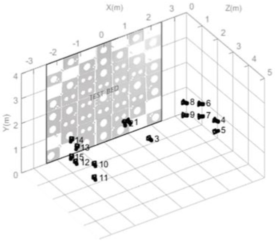
Figure 4. Data acquisition locations for self-calibration.

4.2. System Calibration

The system calibration experiments were initially carried out according to the expression of the geometrical relationship between the sensors (i.e., the one-step and two-step approaches).

More specifically, in the one-step approach, the geometric configurations of the sensors are expressed in the EOPs of the reference sensor (the optical sensor in the present study) and the ROPs between the sensors. In other words, when datasets obtained from n different locations are used for this one-step approach, the geometrical locations of the reference sensor are indicated with n different sets of EOPs (i.e., EOP1, EOP2,…, EOPn), and the locations of the range finder can be indicated with each set of EOPs and 1 set of ROPs which are constant between the optical sensor and the range finder (shown in Figure 5). The values of the EOPs and ROPs are derived directly through a bundle block adjustment procedure.

Figure 5. One-step system calibration.

On the other hand, in the two-step approach, the geometric configurations between the sensors are derived according to the EOPs of the individual sensors. More specifically, the geometrical locations of the sensor system are indicated as n sets of EOPs of the optical sensor and n sets of EOPs of the range finder (refer to Figure 6). These EOPs are derived through a bundle block adjustment procedure. Afterwards, n sets of ROPs are calculated using the derived sets of EOPs of the involved sensors. Finally, a single set of ROPs is calculated by averaging the n sets of ROPs.

Figure 6. Two-step system calibration.

The other important factor that should be considered in system calibration is the datasets’ configurations. First, 11 datasets were acquired using the optical-range-finder system, as seen in Figure 7a,b. The data acquisition locations for the system calibration were selected to have enough number of and even distribution of control points over an entire image. Figure 7a shows layout of data acquisition locations, and Figure 7b shows grouping of the locations. The locations were grouped by row (parallel direction to the testbed plane) and column (orthogonal direction to the testbed plane).

Figure 7. Data acquisition configuration for system calibration: (a) data acquisition locations of sensor system; (b) grouping of the locations.

Afterwards, 46 combinations from the 11 datasets were produced (as seen in Table 2). They are utilized to determine the effects of the number and locations of datasets on the accuracy of system calibration. Again, the datasets were selected while considering the number of datasets (i.e., ranging from 2 to 11 sets), the column selection (i.e., ranging from one column or more than one column), and the convergence (or symmetry) of the datasets. For example, in the case of 2-dataset selection from at least two columns, datasets 2 and 9 (in the second row) can be selected instead of datasets 2 and 5 or datasets 5 and 9.

Table 2. Combinations of datasets based on number and location.

Number of Datasets	Location of Selected Datasets
	One Column	Two or More Columns
2	8 cases (e.g., dataset 5, and 6)	4 cases (e.g., dataset 2, and 9)
3	5 cases (e.g., dataset 5, 6, and 7)	3 cases (e.g., dataset 2, 5, and 9)
4	2 cases (e.g., dataset 1, 2, 3, and 4)	7 cases (e.g., dataset 2, 3, 9, and 10)
5	-	6 cases (e.g., dataset 2, 3, 5, 9, and 10)
6	-	5 cases (e.g., dataset 2, 3, 5, 6, 9, and 10)
8	-	3 cases (e.g., dataset 2, 3, 4, 5, 6, 9, 10, and 11)
9	-	2 cases (e.g., dataset 2, 3, 4, 5, 6, 7, 9, 10, and 11)
11	-	1 case (all dataset)
total	15 cases	31 cases

4.3. Optical and Range-Finder Data Fusion

Using the IOPs and ROPs acquired from the procedures in Section 4.1 and Section 4.2, and together with the collinearity conditions (Equations (1) and (2)), RGB-D data can be created through the optical and range-finder data fusion procedure. More specifically, Figure 8 shows the conceptual idea of the data fusion method. In this figure, P_opt and P_RF are the respective data from the optical and range-finder data. The distortion-free 3D coordinates, (X_df, Y_df, Z_df), can be calculated after removing the range sensor lens distortions, and range distortions from the raw range datasets. Then, the 3-dimentional coordinates w.r.t. the range finder coordinate system can be transformed into the coordinates w.r.t. the optical camera coordinate system using Equation (9). Afterwards, the corresponding image coordinates of the optical camera data can be calculated using Equations (1) and (2) while considering lens distortion effects. Subsequently, the corresponding color (R, G, B) values can be determined for the image coordinates. In this way, RGB-D data can be generated from the optical-range-finder system.

$$\left[\begin{array}{c}{X}_{optic}\\ Y_{optic}\\ Z_{optic}\end{array}\right]=T_{rop}+{(R_{\mathrm{rop}})}^T\left[\begin{array}{c}{X}_{df}\\ Y_{df}\\ Z_{df}\end{array}\right]$$

(9)

where (X_df, Y_df, Z_df) are the coordinates of a certain point in the range finder data after removing distortions. T_rop and R_rop are translation and rotation matrices of ROPs between the optical camera and range finder coordinate systems. (X_optic, Y_optic, Z_optic) are the coordinates of the point w.r.t. the optical camera coordinate system.

Figure 8. Geometric relationship for data fusion using optical-range-finder system.

In this research, the authors dealt with 2 different ways of expressing the geometrical relationship between the sensors (i.e., the one-step and two-step approaches), and 46 combinations of datasets. Accordingly, 92 sets of ROPs and RGB-D datasets were produced from 46 cases with the one-step approach and 46 cases with the two-step approach.

4.4. Proposed Evaluation Strategies

The qualities of the 92 sets of ROPs estimation results were analyzed based on the standard deviations of the estimated parameters. For the case of data fusion results, a measure called matching rate is proposed and utilized in this research. In previous studies, the qualities of the data fusion results were mostly evaluated through visual inspection ([20,22,23,28,29,30]). We have 92 sets of fusion results to be compared each other, a qualitative measure is, therefore, critically necessary for the comparisons. Since the inaccurate data fusion results distinctly appear in the areas where different patches meet each other, the same color value is intentionally assigned into the same patches on the optical and range-finder data, and the color values of the corresponding points are compared. The proposed data fusion evaluation strategy can be explained in detail as follows. First, several regions suitable for quality evaluation were manually selected from the original intensity and optical data (Figure 9a,b). Then, the same color value (user-defined) was assigned for all pixels in the same region on the two images (Figure 9c,d). Lastly, data fusion was carried out with the user-defined color images according to the procedures described previously. In this step, the user-defined colors assigned for the corresponding points (i.e., P_opt and P_RF) were compared. At this stage, inaccurate data fusion will lead to an increased number of mismatching points (i.e., corresponding points with different color values, COLOR_opt ≠ COLOR_RF). The white color value was assigned for mismatching points in the visual investigation (see Figure 10). For quantitative assessment, all points in the evaluation regions and matching points were counted. Afterwards, the matching rate was calculated according to Equation (10).

$$Matching rate=\frac{{{\displaystyle \sum }}_{i=1}^{no of datasets}\frac{no of mathcing points in i^{th} dataset}{total no of points for evaluation in i^{th} dataset}}{no of datasets}$$

(10)

Figure 9. Three datasets for evaluation of data fusion results: (a) raw intensity images; (b) raw optical images; (c) intensity images with user-defined color values; (d) optical images with user-defined color values.

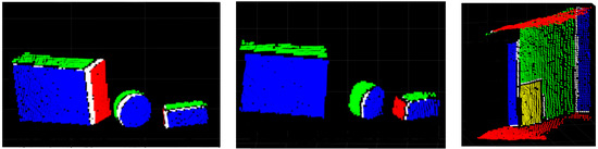
Figure 10. Examples of data fusion results for accuracy evaluation.

As seen in Figure 9 and Figure 10, three datasets were used for the evaluation of data fusion accuracy. These datasets consisted of two datasets in which various objects such as boxes and cylinders were placed and data acquisition locations were differentiated. The third dataset acquired in a corridor was selected for inclusion of indoor elements such as doors, windows, and pillars.

5. Experimental Results and Discussion

Experiments for self-calibration and system calibration for optical and range data fusion were carried out. More detailed explanations of the experimental results are provided in the following sub-sections.

5.1. Self-Calibration Results

Table 3 presents the estimated IOPs from the optical camera and range finder, and Table 4 shows the standard deviations of the estimated IOPs and residual accuracies. The root mean square (RMS) results of the residual values from a bundle adjustment showed 0.38 pixels (0.0025 mm) and 0.76 pixels (0.0305 mm) for the image data from the optical camera and range finder, respectively. The two RMS values for the image data were less than 0.8 pixels. The RMS value for the range data showed 6.84 mm which was better than the nominal value of 1 cm and the results from previous studies that used the same range finder [10,11]. The RMS values of 8.9 mm and 8.1 mm for the cases without and with distortion parameters were shown in [10], respectively. Also, the RMS values ranging from 12.1 mm to 13.0 mm were shown in Ref. [11]. The standard deviations of the estimated IOPs in Table 4 all showed very small amounts compared to the IOPs itself. This means that the precisions of the self-calibration parameters were high. As such, the estimated IOPs from the self-calibration procedure were accurate enough to be utilized in the system calibration.

Table 3. Estimated self-calibration parameters.

Sensors	Estimated IOPs
Optical camera	xp (mm)	yp (mm)	focal length (mm)
	−0.02850	0.01401	34.190
	K1	K2	K3	P1	P2	A1	A2
	−6.3×10−5	2.94×10−8	3.82×10−11	−2.1×10−5	1.5×10−5	−1.4×10−5	5.47×10−5
Range finder	xp (mm)	yp (mm)	focal length (mm)
	0.04607	−0.00513	5.7647
	K1	K2	K3	P1	P2	A1	A2
	0.001093	−0.00255	0.000145	0.000841	−0.0003	−0.00236	0.001952
	d0	d1	e1	e2
	−48.9753	0.022105	2.827089	3.428659

Table 4. Standard deviations of the estimated IOPs and residual accuracies.

Sensors	RMS of Residuals	Standard Deviations of the Estimated IOPs
Optical camera	0.0025 mm (0.38 pixels)	xp (mm)	yp (mm)	focal length (mm)
		0.0007	0.0006	0.0021
		K1	K2	K3	P1	P2	A1	A2
		2.61×10−7	1.23×10−9	1.73×10−12	3.40×10−7	2.69×10−7	6.10×10−6	7.07×10−6
Range finder	0.0305 mm (0.76 pixels)	xp (mm)	yp (mm)	focal length (mm)
		0.0044	0.0039	0.0644
		K1	K2	K3	P1	P2	A1	A2
		6.56×10−5	1.20×10−5	6.72×10−7	4.70e×10−6	5.15×10−6	3.21×10−5	3.19×10−5
	6.84 mm (range)	d0	d1	e1	e2
		2.37	0.0021	0.1823	0.1659

5.2. System Calibration Results

The analysis of the system calibration and data fusion results were performed in three ways: (i) two ROP calculation methods (i.e., one-step or two-step method); (ii) different geometrical locations of datasets (i.e., single or multiple columns); (iii) different numbers of datasets.

First of all, the mean, highest, and lowest values of matching rates were derived from all of the dataset cases while applying either the one-step or two-step method (in Table 5, where the standard deviations of the estimated ROPs also are shown). Overall, the one-step method showed better results than the two-step one in terms of matching rate and parameter precision (i.e., standard deviations of ROPs).

Table 5. Matching rates of fusion data and standard deviations of ROPs.

		Matching Rate (%)	Standard Deviations of ROPs
			X0 (mm)	Y0 (mm)	Z0 (mm)	ω (Degree)	ϕ (Degree)	κ (Degree)
One Step	Mean	97.85	3.27	4.00	1.78	0.07	0.06	0.10	From all 46 cases
	Highest rate	99.08	2.67	3.18	1.49	0.04	0.04	0.08	6 datasets used (from multiple columns)
	Lowest rate	94.7	7.22	8.03	2.86	0.14	0.13	0.15	2 datasets used (from single column)
Two step	Mean	97	22.1	19.93	49.33	0.31	0.40	0.26	From all 46 cases
	Highest rate	98.86	11.55	20.28	53.47	0.40	0.3	0.16	5 datasets used (from multiple columns)
	Lowest rate	92.8	20.00	51.21	0.76	0.53	0.23	0.09	2 datasets used (from single column)

Among the one-step cases, the highest matching rate came from the system calibration performed using six datasets in multiple columns (i.e., columns 1, 2, and 3, and rows 3, and 4; datasets 3, 4, 6, 7, 10, and 11 in Figure 7b). Moreover, this case was the most accurate one among all cases (i.e., 92 cases including the one-step and two-step approaches). The lowest rate was observed for the case using two datasets in a single column (i.e., column 2 and rows 3, and 4; datasets 6, and 7 in Figure 7b).

Considering the two-step cases only, the highest matching rate came from the case using five datasets in multiple columns (i.e., columns 1, 2, and 3, and rows 2, 3, and 4; datasets 3, 5, 6, 7, and 10 in Figure 7b). The lowest matching rate was observed for the same one-step case noted above. The most inaccurate result was shown when two-step calibration was performed using two datasets (i.e., column 1 and rows 2, and 3; datasets 2, and 3 in Figure 7b).

Secondly, the effects of the different geometrical locations of datasets on the matching rate were analyzed. In other words, the mean values and standard deviations of the matching rates derived from the single-column cases (i.e., 15 cases) were compared with those derived from the multiple-column cases (i.e., 14 cases). The comparison was carried out using the combinations having only 2 to 4 datasets, because there were no single-column cases having more than 4 datasets, as seen in Table 2.

As confirmed in Table 6 and Figure 11, the selection of datasets from multiple columns led to higher mean values regardless of the ROP calibration (i.e., one-step or two-step) method. Also, the standard deviations of the matching rates from the multiple columns were lower than those from the single columns.

Table 6. Matching rates according to data locations (single or multiple columns).

	Dataset Location	Matching Rate (%)
		Mean	Standard Deviation
One-step	single	96.72	0.83
	multiple	98.36	0.58
Two-step	single	95.69	1.35
	multiple	97.00	1.02

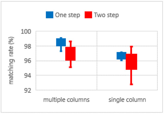
Figure 11. Comparisons of matching rates according to data acquisition locations.

Meanwhile, the standard deviations of the ROPs were derived from bundle adjustment for both the single-column cases (i.e., 15 cases) and multiple-column cases (i.e., 14 cases). Afterwards, the averaged standard deviations were calculated from the single- and multiple-column cases separately. These values are shown in Figure 12a,b; as is apparent, translation parameters (Figure 12a) and rotation parameters (Figure 12b) decreased when the number of columns was increased.

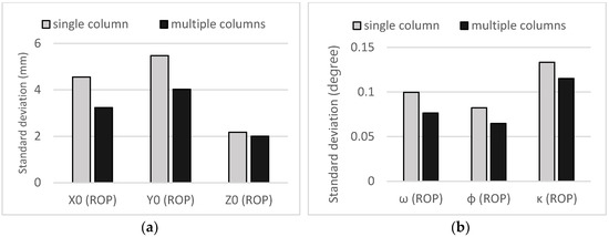
Figure 12. Comparisons of standard deviations of ROPs (results from one-step calibration) according to data acquisition locations: (a) translation (X0, Y0, and Z0); (b) rotation (ω, ϕ, and κ).

Thirdly, the relationship between the number of datasets used and the data fusion and system calibration accuracies was analyzed. At this stage, the combinations of datasets chosen only from the multiple columns (31 cases seen in Table 2) were used, since they showed better results in the previous analysis (in Table 6, Figure 11 and Figure 12).

The mean values and standard deviations of the matching rates according to the different numbers of datasets are shown in Table 7 and Figure 13. For example, 4 combination cases were used to produce a mean value and a standard deviation of matching rate for 2-dataset analysis. As seen in the table and the figure, the relationship between the number of datasets and the mean values of matching rates was not clear in the case of the one-step method. In other words, all of the cases with different numbers of datasets had similar mean values. On the other hand, the deviations of the matching rates showed a different tendency. More specifically, in most cases, the deviation values decreased as the number of datasets was increased, as seen in Table 7 and Figure 13. Using more than four datasets showed a clear trend of reducing standard deviations of matching rates.

Table 7. Mean values and standard deviations of matching rates according to number of datasets.

Number of Datasets (Only from Multiple Columns)		2	3	4	5	6	8+ (8~11)
Mean of matching rates (%)	one-step	98.25	98.31	98.45	98.41	98.38	98.48
	two-step	97.07	95.76	97.44	98.2	98.04	98.25
Standard deviation of matching rates (%)	one-step	0.64	0.76	0.55	0.45	0.48	0.30
	two-step	1.14	0.58	0.72	0.77	0.43	0.23

Figure 13. Comparison of matching rates according to number of datasets.

Meanwhile, firstly, the standard deviations of the ROPs were derived from bundle adjustment for all combination cases of multiple columns (i.e., 31 cases as seen in Table 2); afterwards, the averaged standard deviations were calculated for analysis of different numbers of datasets. For example, 4 combination cases were used to produce an averaged standard deviation for 2-dataset analysis. Figure 14a,b show such values according to the different number of datasets after application of the one-step system calibration approach. As seen in these figure, the increase of the number of datasets used led to a corresponding increase in precision (i.e., a decrease of the standard deviations of ROPs). A particularly notable point in Figure 14 is that the use of at least four datasets largely reduced the range of the standard deviations for the same number of datasets when compared with the use of two or three datasets.

Figure 14. Standard deviations of ROPs according to number of datasets (one-step approach): (a) translation (X0, Y0, and Z0); (b) rotation (ω, ϕ, and κ).

In the case of applying the two-step approach, the use of more than four datasets provided high and stable mean values of matching rate, as seen in Table 7 and Figure 13. Also, the standard deviation analysis of the ROPs (in Figure 15a,b) found that four or more datasets provided more stable standard deviations of ROPs. On the other hand, two and three dataset cases showed unstable results, as seen in Table 7, and Figure 13 and Figure 15. In the table and Figure 13, the mean of matching rates for the case of two dataset (i.e., 97.07%) was higher than the value for the case of three dataset (i.e., 95.76%), However, the standard deviations of the matching rates for these two cases were the other way around. In case of the standard deviations of ROPs as seen in Figure 15, there is discrepancy between the values for two and three dataset cases. The standard deviations for two dataset case were mostly higher than the values for three dataset case. Overall, the accuracy (i.e., matching rate) of the two dataset case is higher than the three dataset case; however, the precision (i.e., standard deviation) is vice versa. Such unstable results might come from low number of datasets and low number of combinations as well (i.e., two datasets with four combinations and three datasets with three combinations). Note that four or more dataset cases have either enough number of datasets or combinations compared to two and three dataset cases.

Figure 15. Standard deviations of ROPs according to number of datasets (two-step approach): (a) translation (X0, Y0, and Z0); (b) rotation (ω, ϕ, and κ).

Comparing Figure 14 and Figure 15, one can see that employing more datasets with the one-step approach has a more obvious positive effect on the standard deviations of ROPs than is the case with the two-step approach.

Additionally, four data fusion results among ninety-two cases were selected and illustrated in Figure 16. Table 5 already includes their matching rates and standard deviations of ROPs. The cases with the highest rate (99.08%) using one-step approach and 6 datasets in multiple columns, lowest rate (94.70%) using one-step approach and 2 datasets in single column, highest rate (98.86%) using two-step approach and 5 datasets in multiple columns, and lowest rate (92.80%) using two-step approach and 2 datasets in single column are shown in the figure. As expected, large white regions indicating mismatching points are shown in Figure 16d–f,j–l for the cases with the lowest matching rates. On the other hand, few numbers of white points are shown in Figure 16a–c,g–i for the cases with the highest matching rates.

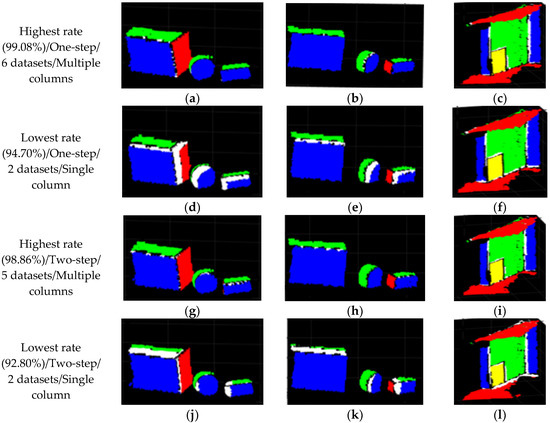
Figure 16. Four data fusion results among ninety-two cases: (a–c) highest rate using one-step approach and 6 datasets in multiple columns; (d–f) lowest rate using one-step approach and 2 datasets in a single column; (g–i) highest rate using two-step approach and 5 datasets in multiple columns; (j–l) lowest rate using two-step approach and 2 datasets in a single column.

6. Conclusions and Recommendations

This study provided and compared various system calibration results comprehensively according to the calibration approach (i.e., one-step or two-step) and the characteristics of the used datasets (i.e., different geometrical locations and number of datasets). Prerequisite accurate self-calibration procedures were performed before system calibration. Afterwards, 46 combinations of datasets were made with 11 datasets, and 92 sets of ROPs were calculated through the system calibration procedures. These sets of ROPs and their corresponding fusion data results were compared comprehensively. First of all, the matching rate and precision derived from the one-step system calibration were generally higher than those from the two-step one. Secondly, the datasets acquired from the converging configuration (i.e., multiple columns) provided better performance than did the other case (i.e., single column). Thirdly, we found that the number of datasets used was highly correlated with the precision of the calculated ROPs in cases where the one-step method was applied. In other words, the deviations of ROPs were decreased when the number of datasets used was increased. Additionally, for either the one- or two-step approach, the use of more than four datasets (from multiple columns) provided high and stable mean values of matching rates and stable standard deviations of ROPs.

Based on a comprehensive analysis of the various experimental results, we can conclude that highly accurate system calibration and data fusion results can be obtained through (1) the use of more than four datasets acquired in converging multiple directions and (2) the execution of one-step system calibration. We can also recommend that increasing the number of datasets (at least four datasets from converging multiple directions) will be advantageous to achieve relatively accurate fusion results.

Overall, this study was conducted in consideration of self-calibration, system calibration, and data acquisition configurations. Based on a comprehensive analysis of the experimental results, guidelines for accurate and efficient derivation of ROP and data fusion results are presented herein. In terms of the applications, the proposed methodology can be utilized for virtual reality, indoor modeling, indoor positioning, motion detection and reconstruction, and so on. Follow-up studies will be conducted to alleviate the range data problems arising from low resolution, noisy range data, multi-path effects, the ambiguity range, scattering problem, and other issues.

References

- Chow, J.C.; Lichti, D.D.; Hol, J.D.; Bellusci, G.; Luinge, H. Imu and multiple RGB-D camera fusion for assisting indoor stop-and-go 3D terrestrial laser scanning. Robotics 2014, 3, 247–280. [Google Scholar] [CrossRef]
- Salinas, C.; Fernández, R.; Montes, H.; Armada, M. A New Approach for Combining Time-of-Flight and RGB Cameras Based on Depth-Dependent Planar Projective Transformations. Sensors 2015, 15, 24615–24643. [Google Scholar] [CrossRef] [PubMed]
- Shim, H.; Adelsberger, R.; Kim, J.D.; Rhee, S.-M.; Rhee, T.; Sim, J.-Y.; Gross, M.; Kim, C. Time-of-flight sensor and color camera calibration for multi-view acquisition. Visual Comput. 2012, 28, 1139–1151. [Google Scholar] [CrossRef]
- Nair, R.; Ruhl, K.; Lenzen, F.; Meister, S.; Schäfer, H.; Garbe, C.S.; Eisemann, M.; Magnor, M.; Kondermann, D. A survey on time-of-flight stereo fusion. In Time-of-Flight and Depth Imaging. Sensors, Algorithms, and Applications; Springer: Berlin/Heidelberg, Germany, 2013; pp. 105–127. [Google Scholar]
- Zhang, L.; Dong, H.; Saddik, A.E. From 3D sensing to printing: A survey. ACM Trans. Multimed. Comput. Commun. Appl. (TOMM) 2016, 12, 27. [Google Scholar] [CrossRef]
- Beyer, H.A. Geometric and Radiometric Analysis of a CCD-Camera Based Photogrammetric Close-Range System; ETH Zurich: Zurich, Germany, 1992. [Google Scholar]
- Brown, D.C. Decentering distortion of lenses. Photogramm. Eng. Remote Sens. 1966, 3, 444–462. [Google Scholar]
- Fraser, C.S. Digital camera self-calibration. ISPRS J. Photogramm. Remote sens. 1997, 52, 149–159. [Google Scholar] [CrossRef]
- Remondino, F.; Fraser, C. Digital camera calibration methods: considerations and comparisons. Int. Arch. Photogramm. Remote Sens. Spat. Inf. Sci. 2006, 36, 266–272. [Google Scholar]
- Lichti, D.D.; Kim, C.; Jamtsho, S. An integrated bundle adjustment approach to range camera geometric self-calibration. ISPRS J. Photogramm. Remote Sens. 2010, 65, 360–368. [Google Scholar] [CrossRef]
- Lichti, D.D.; Kim, C. A comparison of three geometric self-calibration methods for range cameras. Remote Sens. 2011, 3, 1014–1028. [Google Scholar] [CrossRef]
- Lichti, D.D.; Qi, X. Range camera self-calibration with independent object space scale observations. J. Spat. Sci. 2012, 57, 247–257. [Google Scholar] [CrossRef]
- Jamtsho, S. Geometric Modelling of 3D Range Cameras and Their Application for Structural Deformation Measurement. Master’s Thesis, University of Calgary, Calgary, AB, Canada, 2010. [Google Scholar]
- Westfeld, P.; Mulsow, C.; Schulze, M. Photogrammetric calibration of range imaging sensors using intensity and range information simultaneously. Proc. Opt. 3-D Meas. Tech. IX 2009, 2, 1–10. [Google Scholar]
- Lindner, M.; Kolb, A. Lateral and depth calibration of PMD-distance sensors. In Proceedings of the International Symposium on Visual Computing, Las Vegas, NV, USA, 14–16 December 2006; Springer: Berlin/Heidelberg, Germany, 2006; pp. 524–533. [Google Scholar]
- Zhu, J.; Wang, L.; Yang, R.; Davis, J.E. Reliability fusion of time-of-flight depth and stereo geometry for high quality depth maps. IEEE Trans. Pattern Anal. Mach. Intell. 2011, 33, 1400–1414. [Google Scholar] [PubMed]
- Mikhelson, I.V.; Lee, P.G.; Sahakian, A.V.; Wu, Y.; Katsaggelos, A.K. Automatic, fast, online calibration between depth and color cameras. J. Vis. Commun. Image Represent. 2014, 25, 218–226. [Google Scholar] [CrossRef]
- Van den Bergh, M.; Van Gool, L. Combining RGB and ToF cameras for real-time 3D hand gesture interaction. In Proceedings of the 2011 IEEE Workshop on Applications of Computer Vision (WACV), Kona, HI, USA, 5–7 January 2011; IEEE: Piscataway, NJ, USA, 2011; pp. 66–72. [Google Scholar]
- Hansard, M.; Evangelidis, G.; Pelorson, Q.; Horaud, R. Cross-calibration of time-of-flight and colour cameras. Comput. Vis. Image Underst. 2015, 134, 105–115. [Google Scholar] [CrossRef]
- Herrera, D.; Kannala, J.; Heikkilä, J. Joint depth and color camera calibration with distortion correction. IEEE Trans. Pattern Anal. Mach. Intell. 2012, 34, 2058–2064. [Google Scholar] [CrossRef] [PubMed]
- Wu, J.; Zhou, Y.; Yu, H.; Zhang, Z. Improved 3D depth image estimation algorithm for visual camera. In Proceedings of the 2nd International Congress on Image and Signal Processing, CISP′09, Tianjin, China, 17–19 October 2009; IEEE: Piscataway, NJ, USA, 2009; pp. 1–4. [Google Scholar]
- Jung, J.; Lee, J.-Y.; Jeong, Y.; Kweon, I.S. Time-of-flight sensor calibration for a color and depth camera pair. IEEE Trans. Pattern Anal. Mach. Intell. 2015, 37, 1501–1513. [Google Scholar] [CrossRef] [PubMed]
- Vidas, S.; Moghadam, P.; Bosse, M. 3D thermal mapping of building interiors using an RGB-D and thermal camera. In Proceedings of the 2013 IEEE International Conference on Robotics and Automation (ICRA), Karlsruhe, Germany, 6–10 May 2013; IEEE: Piscataway, NJ, USA, 2013; pp. 2311–2318. [Google Scholar]
- Lindner, M.; Kolb, A.; Hartmann, K. Data-fusion of PMD-based distance-information and high-resolution RGB-images. In Proceedings of the International Symposium on Signals, Circuits and Systems, ISSCS 2007, Iasi, Romania, 13–14 July 2007; IEEE: Piscataway, NJ, USA, 2007; pp. 1–4. [Google Scholar]
- Borrmann, D.; Afzal, H.; Elseberg, J.; Nüchter, A. Mutual calibration for 3D thermal mapping. IFAC Proc. Vol. 2012, 45, 605–610. [Google Scholar] [CrossRef]
- Munaro, M.; Basso, F.; Menegatti, E. OpenPTrack: Open source multi-camera calibration and people tracking for RGB-D camera networks. Robot. Autonomous Syst. 2016, 75, 525–538. [Google Scholar] [CrossRef]
- Mikhail, E.M.; Bethel, J.S.; McGlone, J.C. Introduction to Modern Photogrammetry; John Wiley and Sons, Inc.: New York, NY, USA, 2001. [Google Scholar]
- Owens, J.L.; Osteen, P.R.; Daniilidis, K. MSG-cal: Multi-sensor graph-based calibration. In Proceedings of the 2015 IEEE/RSJ International Conference on Intelligent Robots and Systems (IROS), Hamburg, Germany, 28 September–2 October 2015; IEEE: Piscataway, NJ, USA, 2015; pp. 3660–3667. [Google Scholar]
- Shin, Y.-D.; Park, J.-H.; Bae, J.-H.; Baeg, M.-H. A study on reliability enhancement for laser and camera calibration. Int. J. Control Autom. Syst. 2012, 10, 109–116. [Google Scholar] [CrossRef]
- Wang, W.; Yamakawa, K.; Hiroi, K.; Kaji, K.; Kawaguchi, N. A Mobile System for 3D Indoor Mapping Using LiDAR and Panoramic Camera. Spec. Interest Group Tech. Rep. IPSJ 2015, 1, 1–7. [Google Scholar]
© 2018 by the authors. Licensee MDPI, Basel, Switzerland. This article is an open access article distributed under the terms and conditions of the Creative Commons Attribution (CC BY) license (http://creativecommons.org/licenses/by/4.0/).