Improved Jitter Elimination and Topology Correction Method for the Split Line of Narrow and Long Patches

Abstract

Extracting the split line of narrow and long patches is important for the generalization of land-use thematic data. There are two commonly used methods for extracting the split lines: One is based on Delaunay triangulation and the other is based on straight skeletons. However, it is difficult for the straight skeleton method to preserve geometric structure and topological consistency with the original data when dealing with polygons that have irregularity and complexity of junctions. Therefore, we propose an improved jitter elimination and topology correction method for split lines based on a constrained Delaunay triangulation. First, a split line adjustment algorithm based on the geometric structure of the polygon is proposed to eliminate the jitters. Second, a split line topology correction algorithm is proposed for nodes with degree 1 or degree 2, considering the boundary topological constraint. The reliability of the proposed method is verified by comparing it with the straight skeleton method using sample data and the superiority of the proposed method is verified by using actual data from China’s geographical conditions census in the Guizhou province.

1. Introduction

According to Van Oosterom [1] and Beard and Mackaness [2], split line plays an important role in maintaining the complete coverage and non-overlapping spatial characteristics of patch data before and after their generalization, because it is the key element in the collapse and dissolve operators for patch polygons. However, extracting the patch split line accurately and effectively is still a difficult problem [3], especially in the case of irregularly shaped patches, such as small patches as well as long and narrow patches. This study focuses on the extraction, jitter elimination, and topology correction algorithms for the split line of long and narrow patches.

A long and narrow patch refers to a polygon object with a rather large length and small width, such as slender rivers, low-grade roads and highways, and ridges and ditches. In general, a long and narrow patch connects patches of different land feature types and is an important map element for maintaining and ensuring connectivity among patches. According to the definition of fine bending given by Mitropoulos et al. [4], the width of long and narrow patches can be calculated by the following equation: $W=S/BL$, where W is the approximate average width of the patch, S is the patch area, and BL is the lengthwise baseline determined by the longest skeleton line in the patch. According to the roughness of the drawing pen and the resolution of the human eye, Muller [5] defines 0.4 mm as the minimum distance of the visual resolution on the map, so when the width W of a long and narrow patch, such as a road, river, canal, or trench, is under 0.4 mm, the planar patch can be treated as a long and narrow patch.

Splitting a long and narrow patch has been studied when generalizing land use data, with the skeleton line of the patch as the primary split line. There are many research works on the generation of skeleton lines, and skeleton line calculation algorithms based on basic geometric shapes, such as the Voronoi diagram and Delaunay triangulation, are very effective. However, although a split line is constructed based on the skeleton line, it is different from a skeleton line because it not only expresses the main shape of the objects but also takes into account the spatial structure and topological relations of the objects. As such, this paper proposes an improved jitter removal and topology correction method for split line of long and narrow patches. Our method optimizes the consistency of structural characteristics and the topological relationship to produce split lines in accordance with a human’s cognition.

The remainder of this paper is organized as follows. Section 2 reviews the related works on split line extraction. Section 3 analyzes the advantages and disadvantages of the straight skeleton method and its optimization. Section 4 describes our improved split line extraction method with the constrained Delaunay triangulation (CDT), achieving split line jitter removal and topology correction. Section 5 demonstrates the experiments and analyses. Section 6 presents the discussion and conclusions.

2. Related Works

Skeleton extraction operators may be divided into two types according to different source data: Raster-based and vector-based skeleton extraction methods. This study falls in the latter category. At present, three methods are used to extract the split lines in the long and narrow patch, namely rounded skeleton lines, straight skeleton lines, and triangulation-based skeleton lines.

• Rounded skeleton lines. Lee [6] and Montanari [7] proposed rounded skeleton line methods, i.e., medial axis splitting methods. These rounded skeleton lines are calculated using a Voronoi diagram of the polygon boundary and its vertices. Rounded skeleton lines consist of two parts, namely parabolas and straight lines. The parabolas make the lines smoother at polygon bends. However, this algorithm is considerably complex in design. Consequently, it is difficult to optimize the structural characteristics of the geographic features further.
• Triangulation-based skeleton lines. Owing to the excellent properties of Delaunay triangulation, such as proximity, optimality, regionality, and convexity polygons [8,9], scholars have performed considerable research [10,11,12] on the extraction of polygon skeleton lines based on Delaunay triangulation as well as the practical applications. DeLucia and Black [13] first proposed the extraction of polygon skeleton lines based on a CDT and classified the triangles in the triangular mesh into three categories based on the number of polygonal edges present at the three sides of a triangle. Skeleton line extraction for each type of triangle was described, and this formed the foundation for subsequent research.

Li [14] classified the skeleton nodes in Delaunay triangulation, and tracked the main skeleton line of the polygon to reflect the representative shape features and main extension direction of the polygon. Zou and Yan [15] used the CDT to construct the skeleton for polygons and proved that the method was effective. However, Morrison and Zou [16] supposed that the method proposed by Zou and Yan [15] sometimes produces triangles that do not represent the true nature of the underlying shape; therefore, they put forward an improved algorithm by inserting new triangulation points in strategic locations in end, normal, and junction triangles.

As noted by Penninga et al. [17], the direct extraction of skeleton lines with the boundary-CDT suffers from at least the following three drawbacks: (1) skeleton lines at the branch junctions appear to be sawtooth-like; (2) tiny bumps at the boundary lead to extraneous ‘spiked’ skeleton lines; (3) fewer boundary nodes result in the elongation and skewing of skeleton lines. To solve the third problem, Uitermark et al. [18] and Penninga et al. [17] suggested constructing a conformal constrained Delaunay triangulation (CCDT) by addition of Steiner nodes to the boundary. Uitermark et al. [18] also tackled the second problem by boundary simplification, however, this led to the topology error of boundary intersection. Penninga et al. [17] instead tried to solve the second problem by setting a minimum area threshold for the triangles to remove the tiny bumps along the boundary, and they achieved good results. Regarding the first problem, Jones et al. [19] study the ‘T’-shaped junction, and they noted that insofar as there is only one type III triangle present, this triangle can be adjusted by calculating the direction of the three associated skeleton line branches. However, this method cannot be used on ‘+’-shaped branches that have two adjacent type III triangles. On this issue, Penninga et al. [17] proposed connecting the four skeleton line branches to the midpoint of the common edge of two type III triangles for skeleton adjustment, which better solves this type of problem in the ‘+’-shaped junction. In addition, some research has focused on dealing with the ‘X’- and ‘Y’-shaped junction [20]. Nevertheless, the existed research could only solve the relatively simple problems of the skeleton lines extracted by Delaunay triangulation; there are few methods for junctions with complex features, such as multiple type III triangles or skeleton line branches in different directions.

• Straight skeleton lines. Aichholzer et al. [21] proposed a straight skeleton line construction method; the skeleton lines extracted using this method are structurally simple, containing only line segments. The initial algorithm is only applicable to simple polygons. Das et al. [22] extended the scope of the algorithm to the monotone polygon. A simple polygon P is said to be monotone with respect to a line L if its intersection (if any) with any line perpendicular to L is connected. Eppstein and Erickson [23] improved the efficiency of the algorithm by using a technique developed by Eppstein for maintaining the extreme of binary functions.

Haunert and Sester [24] applied the straight skeleton algorithm to solve the problem of area collapse generalization, which refers to geometry type changes from area to line for geographic dare multiple representation. The results of their study showed that the straight skeleton is a powerful tool for the generalization of areas. Furthermore, Haunert and Sester [25] compared the generation results of the three above-mentioned types of skeleton lines and highlighted the advantages of straight skeleton lines when treating split line jitter and redundant split line interference in their extraction. Straight skeletons have good geometric properties and computational efficiency. As such, straight skeleton lines are better suited to the extraction of a patch split line. Furthermore, Haunert and Sester [25] studied dimension-reduction in long and narrow patches using straight skeleton lines, and amended the convergence of multiple nodes in roads, enabling the application of straight skeleton lines to simple polygon splitting.

The triangulation-based skeleton line method and the straight skeleton line method are the two commonly used methods for extracting the split lines; Haunert and Sester [25] suggested that the latter method is better suited to the extraction of a patch split line. However, there are still many complex situations that are difficult to deal with. To illustrate this, the advantages and disadvantages of the straight skeleton line method and its optimization are further analyzed in Section 3. To alleviate the limitations of the straight skeleton line method, the improved split line extraction method with the CDT is proposed in Section 4.

3. Advantages and Disadvantages of Straight Skeletons

Straight skeleton lines are a common method for extracting the split line of narrow and long polygons. Previous studies have shown that the straight skeleton is a powerful and flexible tool for the area collapse algorithm and preserves topological relationships. However, this method leads to inaccurate generalization results in the case of irregularity and complexity of junctions. In this section, we discuss the systematic analysis of the advantages and disadvantages of the straight skeleton algorithm and its improved version.

The formation of a straight skeleton can be regarded as an inward contraction process of the sides of a polygon at a constant rate. Edge collisions during the contraction process are treated by edge events and segmentation events, eventually forming a skeleton composed of vertex angle bisectors of the polygon, as shown by the thick line in Figure 1.

Figure 1. Straight skeletons.

3.1. Original Method for Straight Skeletons

3.1.1. Advantages

Split lines extracted based on the straight skeleton method have the following advantages: (1) each line segment of the straight skeleton is the longest line segment found on the polygon medial axis and (2) no extraneous spikes are generated near the boundary of the polygon in the formation of a straight skeleton. As shown in Region A of Figure 1, when a slight jitter appears at the polygon boundary, the straight skeleton formed describes the jitter well without producing extra spikes. The two advantages noted above make straight skeleton lines a good reflection of the main structural characteristics of polygons, and suitable for extracting split lines in more regular, simple polygons.

3.1.2. Disadvantages

The extracted straight skeleton lines cannot be directly used as split lines for actual geographic objects, including roads and river systems, which often have complex structural characteristics, because these are not visually pleasing. Haunert and Sester [25] discussed three key problems with straight skeletons in a detailed manner. As shown in Figure 2, the thicker line in the figure is the split line which is extracted from the straight skeleton lines. First, there are many branches at the boundary between two geographic objects. When two-dimensional (2D) long and narrow area geographic elements are reduced to 1D line elements with these primary straight skeletons, the topological relation between two neighboring adjacent geographic objects (polygons) cannot be preserved, as shown in Figure 2a. Second, multiple nodes are present in certain parts of the objects (such as corners) at a close distance. The straight skeletons extracted in these regions will be considerably dense. As shown in Figure 2b, there are a large number of skeletons in Box B at the bend. Third, as the branches (three or more) of multiple geographic objects converge, more connecting nodes appear, leading to jitter in the straight skeleton of this region, which does not correspond to the primary shape of the actual geographic objects, as shown in Figure 2c.

Figure 2. Problems with extracting straight skeletons: (a) changes to the topological relation at the end, (b) dense straight skeletons and (c) jitter at the branch junctions.

3.2. Optimization Method for Straight Skeletons

A topologically constrained correcting algorithm, a skeleton elimination algorithm, and a connection point reconstruction algorithm were proposed by Haunert and Sester [25] for the aforementioned three problems, respectively, to optimize a straight skeleton line.

3.2.1. Topologically Constrained Correcting Algorithm

Regarding the difficulty of topological preservation at the boundary between two adjacent geographic objects with directly extracted straight skeletons, Haunert and Sester [25] proposed modifying the inclinations of the planes that define the skeleton to optimize the skeleton. Figure 3a is the optimization result of Figure 2a. The optimized straight skeleton guarantees the uniqueness and integrity of the split line, and also the same topological relationship between adjacent map objects.

Figure 3. Optimization of straight skeletons in Haunert and Sester [25]: (a) topologically constrained correcting algorithm, (b) skeleton elimination algorithm and (c) connection point reconstruction algorithm.

3.2.2. Skeleton Elimination Algorithm

The skeleton elimination algorithm is essentially an iterative deletion of leaf nodes (hanging nodes) in the skeleton lines until the remaining straight skeleton is the medial axis of the polygon. To avoid excessive or insufficient removal of nodes, the skeleton arcs associated with the nodes are constrained in terms of length, width, and angle. Figure 3b shows the elimination results from the dense skeleton lines in Figure 2b. No redundant hanging arc exists in the skeleton line after this elimination.

3.2.3. Connection Point Reconstruction Algorithm

The connection point reconstruction algorithm optimizes the straight skeleton by joining regions where three or more skeleton branches intersect and aggregates these intersections to a single connection point. The summed square of the horizontal distance between this connection point and other intersects must not exceed 3 m [25]. Figure 3c shows the adjustment of the complex merging situation in Figure 2c, with a more prominent primary shape of the optimized skeleton and a smoother connection between skeleton lines as they merge, enhancing the readability of the map.

3.2.4. Existing Problems in the Optimization Method

The optimized straight skeleton is apt for the split line. However, some shortcomings still exist. First, the structural characteristics of the branch junctions are not well preserved. The method proposed by Haunert and Sester [25] directly aggregates the intersections in the branch junctions to a single connection point, with a suitable fitting outcome for linearly extending branches with jitter. However, this method is not applicable to the branch junctions that are morphologically complex with disturbance features. The structural description of these junctions with this method is ambiguous and cannot represent complex structures well. For instance, the solid thick lines in Figure 4b are the skeletons extracted for the road intersection in Figure 4a with the straight skeleton method, which treats the branch skeletons in the junctions as linearly extending straight lines. For case 1, if the total skeleton length in the type II triangles between the two branch nodes is less than a width threshold, and the distance between the intersection points of extended branch lines is less than the width threshold in each aggregation region, Figure 4b looks much better than Figure 4c. However, for case 2, if the total skeleton length in the type II triangles between the two branch nodes is larger than a width threshold and the distance between the intersection points of extended branch lines is larger than the width threshold, on the basis of references [17,25], the local structural feature is very important, which can’t be ignored, Figure 4c is much better than Figure 4b, which reflect accurately the nature of the object. The structural features shown by the solid thick lines in the rectangle in Figure 4c should be retained.

Figure 4. Retaining the structural features of the branch junctions: (a) branch junctions, (b) skeleton lines extracted with Haunert and Sester (2008) and (c) medial axis of the branch junctions.

Moreover, no consideration is given to nodes with degree 2 on the straight skeleton. The concept of the degree of a node comes from graph theory and is defined as follows:

Definition 1.

The out-degree (OutDeg) of a node is the total number of arcs coming out of the node.

Definition 2.

The in-degree (InDeg) of a node is the total number of arcs terminating at the node.

Definition 3.

The degree of a node (Deg) is the sum of its Outdeg and Indeg.

Haunert and Sester [25] defined the degree of all nodes on the straight skeletons of a polygon as follows: The degree of the nodes connected to the boundary is 1, because each node is related to only one arc of the main skeleton, and the degree of the nodes inside the polygon is greater than 3, because these nodes were formed by edge events and segmentation events; they are associated with at least three arcs of the main skeleton. Based on this analysis, the method by Haunert and Sester [25] does not consider nodes with degree 2 on the polygon straight skeleton. Thus, only simple polygons with no self-intersection can be treated by the method. However, thematic land-use data come in various shapes and self-intersection areas are inevitable during the process of collapse and split operations for narrow and long patches with different semantic attributes. Some nodes are thus shared by boundaries extending in different directions, as shown in Figure 5.

Figure 5. Nodes with degree 2.

In Figure 5, Node O, which is on the boundary of the polygon, is the intersection point of four adjacent arc segments: OA, OB, OC, and OD. In theory, the rational split line of this polygon should be the same as the thick line in Figure 5. Node O is associated with two arc segments, OE and OF, of the straight skeleton. Hence, the degree of Node O is 2. However, the method by Haunert and Sester 25 cannot provide the arc segment OF for the straight skeletons.

4. Improved Jitter Elimination and Topology Correction Method for the Split Line

In light of the shortcomings in dimension-reduction (partitioning and merging) of long and narrow polygons using a straight skeleton and its optimization, this paper proposes an improved split line extraction method with the CDT, achieving split line jitter removal and topology correction based on geometrical features and topological constraints, respectively.

4.1. Delaunay Triangulation

Skeleton line construction with the CDT is another method for split line extraction, and considerable research has been carried out in this field. Triangles in a Delaunay triangular network can be divided into three classes—type I, type II, and type III—based on the number of their neighboring triangles in the polygon [13].

Type I triangles have only one adjacent triangle. The two sides of type I triangles are the boundaries of the polygon. Examples are △ABG, △CDE, and △EFG in Figure 6 in which vertices A, D, and, F are the end points of the skeleton lines. Type II triangles have two adjacent triangles. They are the backbone of the skeleton lines, describing the extension direction of original polygon, such as △BCE in Figure 6. The skeletons of type II triangles are unidirectional. Further, Type III triangles have three adjacent triangles; they are located at the intersection of the skeleton branches, which is the origin from where the lines extend in three directions. One example is △BEG in Figure 6, where the branches extend in three directions at Point L.

Figure 6. Delaunay triangle classification.

The Delaunay triangulation method extracts the medial axis for the three types of triangles in the following ways and connects the medial axis to form the skeleton line. The common edge of two adjacent triangles is called the adjacent edge.

With type I triangles, the midpoint of the only adjacent edge is connected to its corresponding vertex, such as in lines AH, DJ, and FK in Figure 6. With type II triangles, the midpoints of two adjacent edges are connected, such as line IJ in Figure 6. With type III triangles, the center of gravity and the midpoints of the three sides are connected, such as lines LI, LK, and LH in Figure 6.

Steiner nodes are some additional nodes which are used to increase the node density between adjacent nodes with larger distances. These nodes need to be added around the boundary of each polygon when constructing the triangulation network for narrow and long patches. This is because the original nodes are often used to describe important morphological characteristics of the polygons, e.g., inflection nodes and intersection nodes. However, as the nodes are generally smaller, the triangles are stretched toward these points when constructing triangulation. As Delaunay triangulation consists of more nodes, and thus more triangles, the resulting skeleton is expected to be smoother. The specifics of this procedure are as follows: First, a densification step, D, is defined, where D is equal to 0.4 mm or a multiple of 0.4 mm. In this study, we use 1.6 mm (4 × 0.4 mm) as a D value. Sampling is then performed between two original nodes in spacing of D to obtain the Steiner points, as shown in Figure 7.

Figure 7. Adding Steiner nodes: (a) Original nodes of area elements and (b) Steiner nodes.

4.2. Split Line Jitter Removal Based on Geometric Features

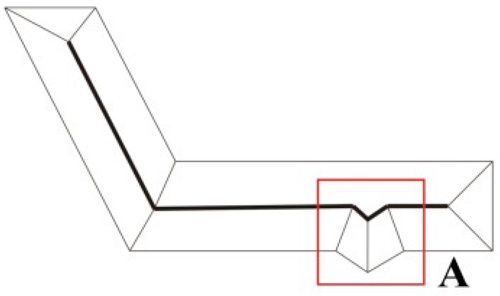
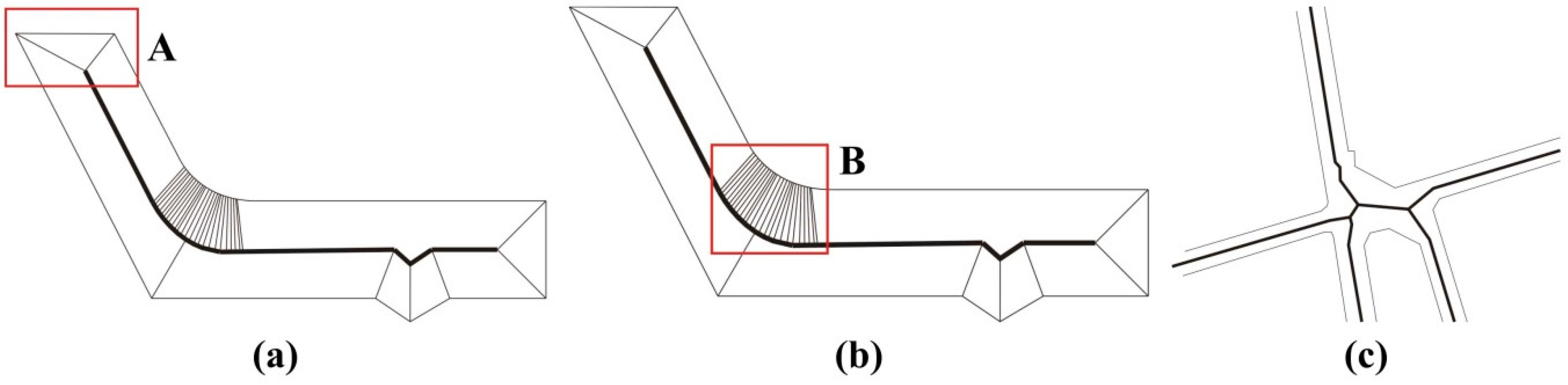
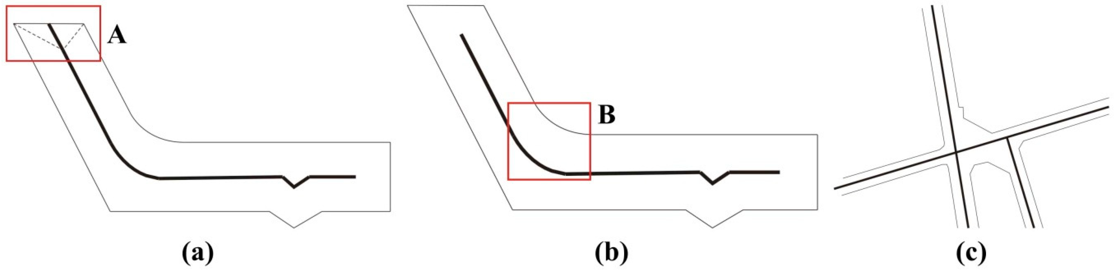
4.2.1. Spike Jitter Adjustment Algorithm

The most pressing problem of split line extraction with Delaunay triangulation is that if the polygon boundary is not considerably smooth, the jitter will be amplified on the split lines even in the case of a slight jitter, thus forming spikes that are difficult to eliminate; for example, the skeleton line shown in box A of Figure 8a.

Figure 8. Spike jitter adjustment algorithm: (a) spike jitter and (b) adjustment result of spike jitter.

The cause for spike jitter (see Figure 8a) lies in the extraction method for type III triangle skeleton lines; i.e., the center of gravity is taken as the central point of the triangle and is connected to the midpoints of the three edges to form the skeleton line. In this manner, when tiny and sharp triangles appear on the polygon boundary, the lines connecting the center of gravity and the midpoints of the two edges will be offset, resulting in the deviation of the skeleton formed from the original extension direction. Therefore, we propose an algorithm to correct for the spike jitter by finding an alternative triangle center.

The basic idea of finding an alternative triangle center is firstly to arrange the length of the three edges of a type III triangle with jitter. The order in ascending length consists of three edges: The shortest side (SS), the middle side (MS), and the longest side (LS). If the SS and the MS are approximately equal in length (SS ≈ MS), the LS is marked. If the MS and the LS are approximately equal in length (MS ≈ LS), the SS is marked. If none of the above conditions is met, no action is taken. The length difference between the two sides must be less than the minimum visually distinct distance of 0.4 mm if it is to be called approximately equal. Connect the midpoint of the marked edge and its corresponding vertex. Then, the midpoint of the connecting line is taken as the alternative center of the type III triangle, which is joined to the midpoints of the two unmarked edges to form the skeleton line, as shown in Figure 8b.

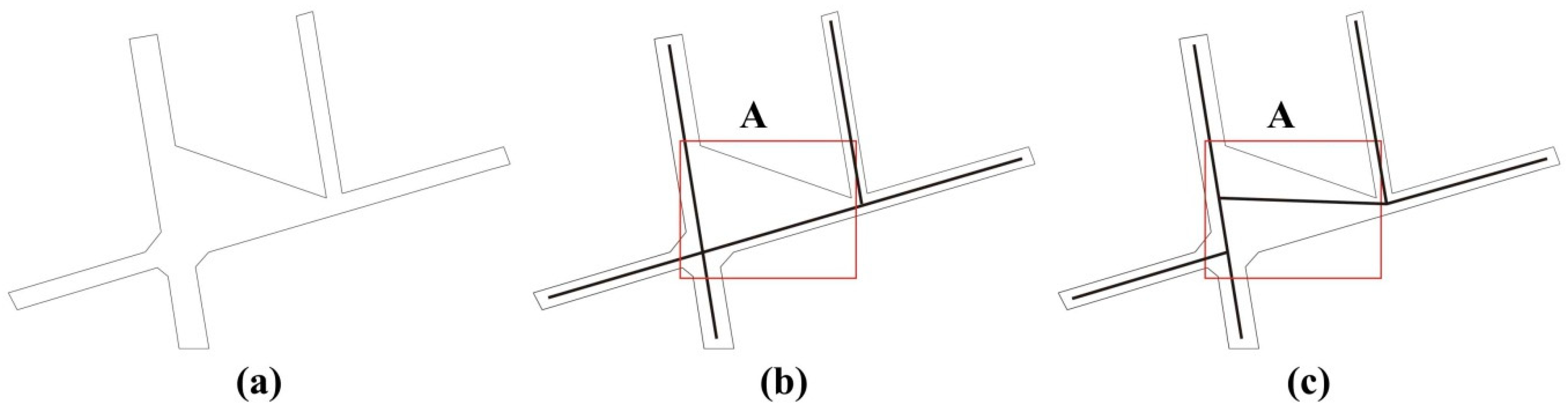
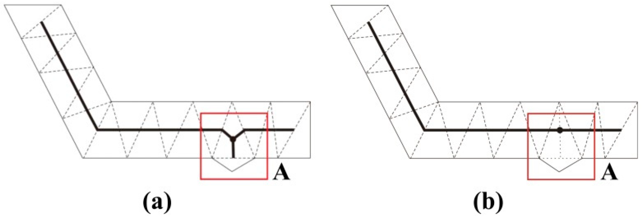
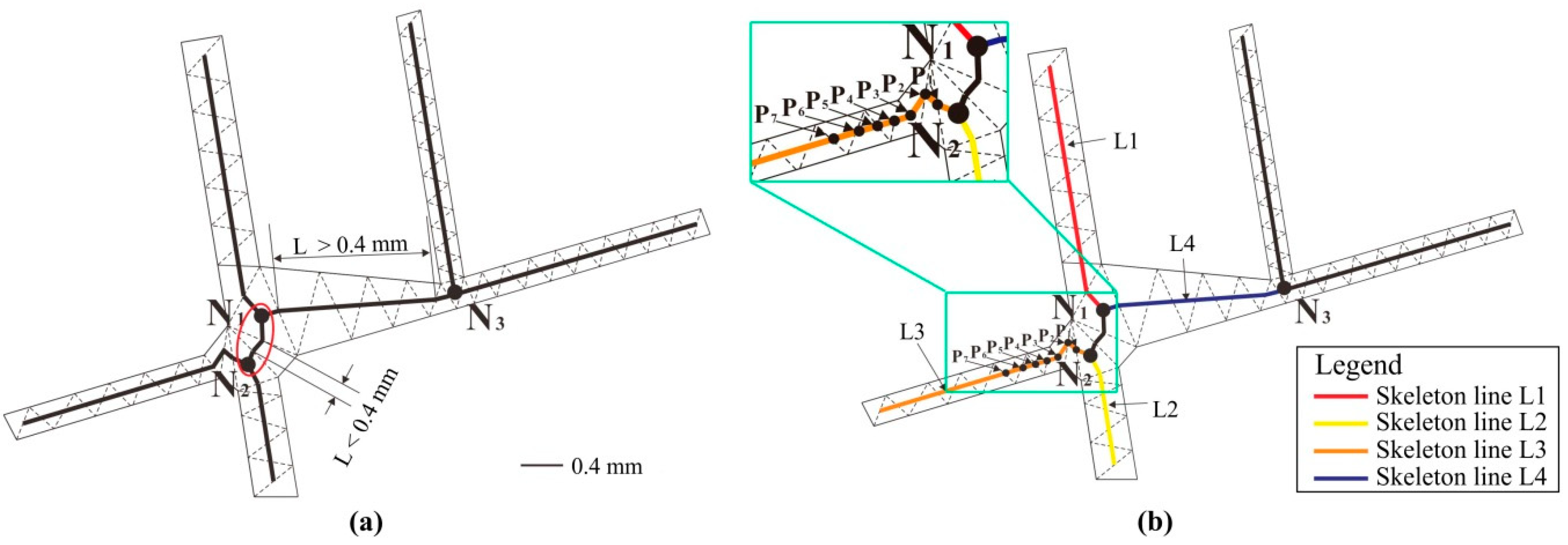
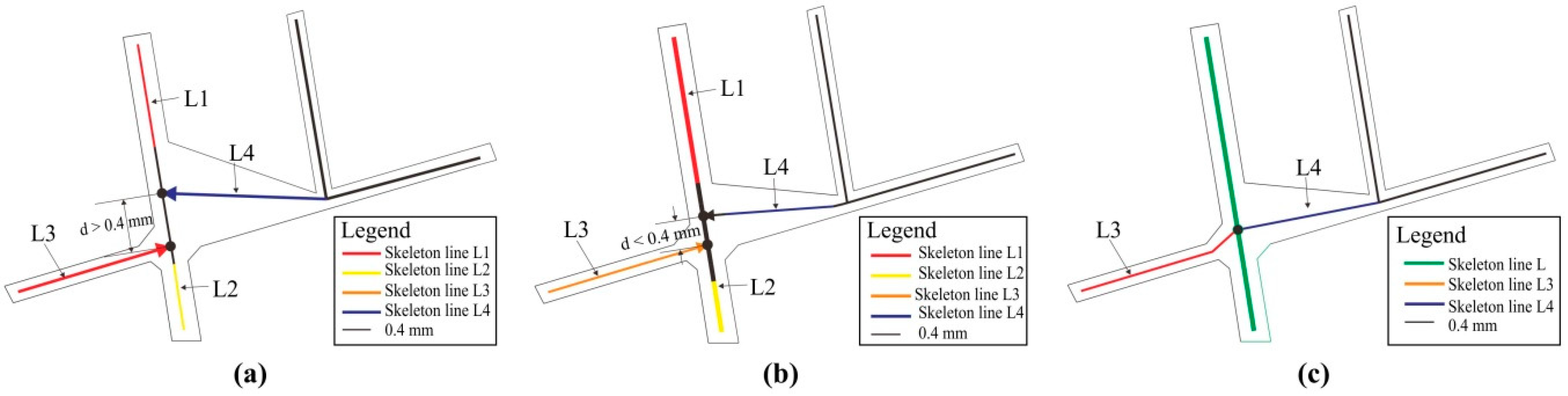
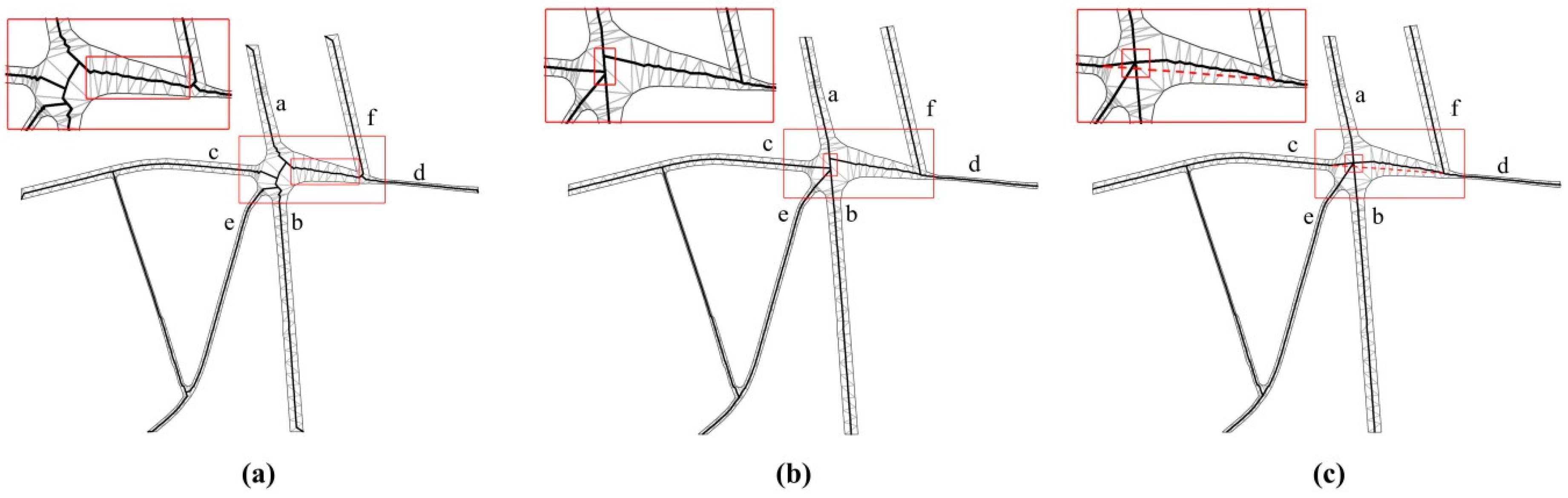
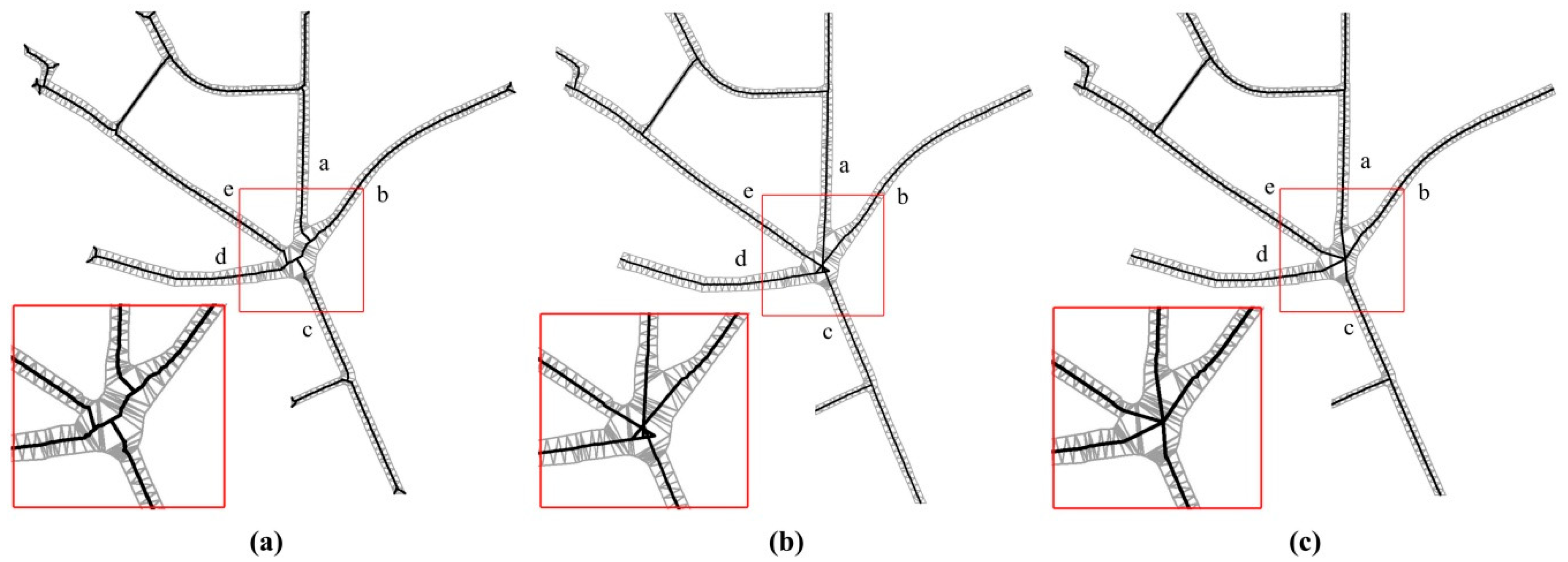
4.2.2. Jitter Adjustment Algorithm for the Branch Junctions

The key to skeleton line extraction at the branch junction region is to maintain local structural features, which involves preserving the linear extension of each skeleton line branch and ensuring the shape consistency between the skeleton line of this region and the actual geographic object. The following algorithm is thus proposed to correct the jitter at the branch convergence region of any arbitrary shape.

Step 1: Identifying the branch junctions. The topological relation between nodes and arcs is established for the polygon skeleton line in the area to be generalized, and the branch junctions are identified according to the degree of the nodes. Dangling nodes are first removed from the topology for more accurate and efficient identification. The retained nodes and arcs are used as the candidate set; if there exist any nodes whose Deg_node ≥ 3, then the node’s location is identified as the branch junction. Type III triangles containing these nodes are also noted.

Step 2: Determining the aggregation zone. In an actual cartographic database, several type III triangles can be adjacent, giving rise to dense branch nodes; or they can be far apart, leading to dispersed branch nodes. Therefore, the adjustment scope for each branch node (i.e., the node aggregation zone) needs to be determined before the skeleton is adjusted in a branch junction for geographic objects at any location. This scope can be determined by the skeleton length between two branch nodes. In this study, two branch nodes form the initial boundary of an aggregation region when the total skeleton length in the type II triangles between them is less than a width threshold (of 0.4 mm). All other nearby branch nodes fulfilling this aggregation criterion are placed at the boundary point set, and they together form the aggregation zone. All nodes, including the branch nodes, are marked as fitting nodes. If the total skeleton length in the type II triangles between two branch nodes is more than or equal to 0.4 mm, the skeleton line segment describes a geographic structure that cannot be directly incorporated, and the skeleton needs to be retained.

As shown in Figure 9a, only one type II triangle is present between branch nodes N1 and N2, and its skeleton length is below the width threshold of 0.4 mm. The two nodes therefore constitute an aggregation region (oval area), whose interior nodes are all fitting nodes. Multiple type II triangles exist between branch nodes N1 and N3, with the total skeleton length above 0.4 mm. These skeleton lines are then kept.

Figure 9. Two key steps in the jitter adjustment algorithm for the branch aggregation region: (a) defining the aggregation region and (b) computing skeleton line direction.

Step 3: Node fitting in aggregation region. Direction consistency is an important condition for the conformance of the skeleton extracted to visual perception rules; however, less attention is paid to this in the existing literature. Haunert and Sester [25] stipulated that if three or more skeleton lines are extended to one point, then that point is the fitting node. However, such a strong constraint is unsuitable in situations with complicated branch junctions. Thus, according to our proposal, the nodes in the fitting region are aggregated considering the direction of nearby skeleton lines, such that if the difference between the azimuth angles of two skeleton lines at a branch node is less than the angle threshold (${\delta }_{angle}$), the two lines are said to be in the same direction. According to a large number of experiments, this value of ${\delta }_{angle}$ is set to 5 degrees in this article. The following algorithm is suggested for nodes fitting in the aggregation region, according to the skeleton line direction features:

(1)

Branch skeleton lines with the same direction are connected preferentially to a straight line. The other branch skeleton lines are extended to this straight line along their respective directions.

(2)

If two skeleton lines which are in the same direction did not exist, the Euclidean distance between the nodes is taken as a similarity measurement. The fitting node is aggregated to the geometric center of the aggregation zone. The branch skeleton lines then are connected to the fitting nodes along their respective directions.

Two key problems are encountered here: The calculation of the skeleton line direction and the re-aggregation of the extension lines. The skeleton line direction refers to its main extension direction, which, in the triangular network, is the steady direction formed by the nodes in type II triangles next to type III ones. However, as type III triangle are usually found in the branch junctions, the direction formed by neighboring type II triangles at a bend cannot represent the direction of the branch skeleton line well. The large number of nodes at the boundary result in dense type II triangles, and the length of their skeleton lines is usually less than the distance of node encryption distance (D). If the skeleton line length in type II triangles is less than the distance threshold (${\delta }_{TD}$), it was recognized and filtered as skeletons at bends. The value of ${\delta }_{TD}$ is set to 1/4D in this article.

For any type III triangle, the type II triangles connected to it are recognized by adjacency. The azimuth and length of each type II triangle are calculated in order. If the skeleton line of a type II triangle Li < TD, the triangle is filtered until four consecutive triangles are found with a uniform skeleton line direction, where L_i ≥ TD. The direction is taken as the skeleton line direction. If, after a certain number of type II triangles are computed, the four triangles determining the direction are still not found, the overall curvature of the branch skeleton is said to be large. At this time, the direction of the four triangles closest to the type III triangle is taken as the skeleton line direction.

As shown in Figure 9b, points P1 and P2 on skeleton L3 are around a bend. The type II triangles they belong to are filtered because they cannot form a uniform skeleton line direction, and the direction of arc segments formed by P3, P4, P5, P6, and P7 meets the aforementioned requirements; therefore, it is used as the skeleton direction, with P3 as the starting node of the direction.

When the aggregation region is sufficiently wide, extending along the respective directions to merge the branch skeletons will not guarantee the intersection of extended branch lines at the same point. Therefore, the nodes of extension lines closer to each other need to be re-aggregated if the distance between two of them is lower than the minimum width threshold. Because the points are on the same straight line, this re-aggregation is performed by fitting each to the node based on their average on the horizontal axis. As seen in Figure 10, skeleton lines L1 and L2 have an identical direction and are preferentially connected to form a straight line, with the other branches extending to it. In Figure 10a, the distance between the intersection points of skeleton lines L3 and L4 is greater than 0.4 mm, so the structure remains unchanged. In Figure 10b, the distance between the intersection points of skeleton lines L3 and L4 is less than 0.4 mm, so it is fitted to the middle node, as shown in Figure 10c.

Figure 10. Re-aggregation of extended lines: (a) inter-node distance > TD, (b) inter-node distance < TD and (c) re-aggregated the skeleton line.

4.3. Split Line Topology Correction

To seamlessly partition long and narrow patches, the following topological constraints at the polygon boundary must be imposed: (1) every split line needs to terminate at a boundary node of the adjacent polygon and (2) the boundary nodes of every neighboring polygon must coincide with a split line end point. The interior split lines of a polygon extracted with Delaunay triangulation should not stretch to the patch boundary. Otherwise, external skeleton lines will fail to link to the interior lines, resulting in a topological difference between the extracted skeleton lines and original map, which then requires split line topology correction.

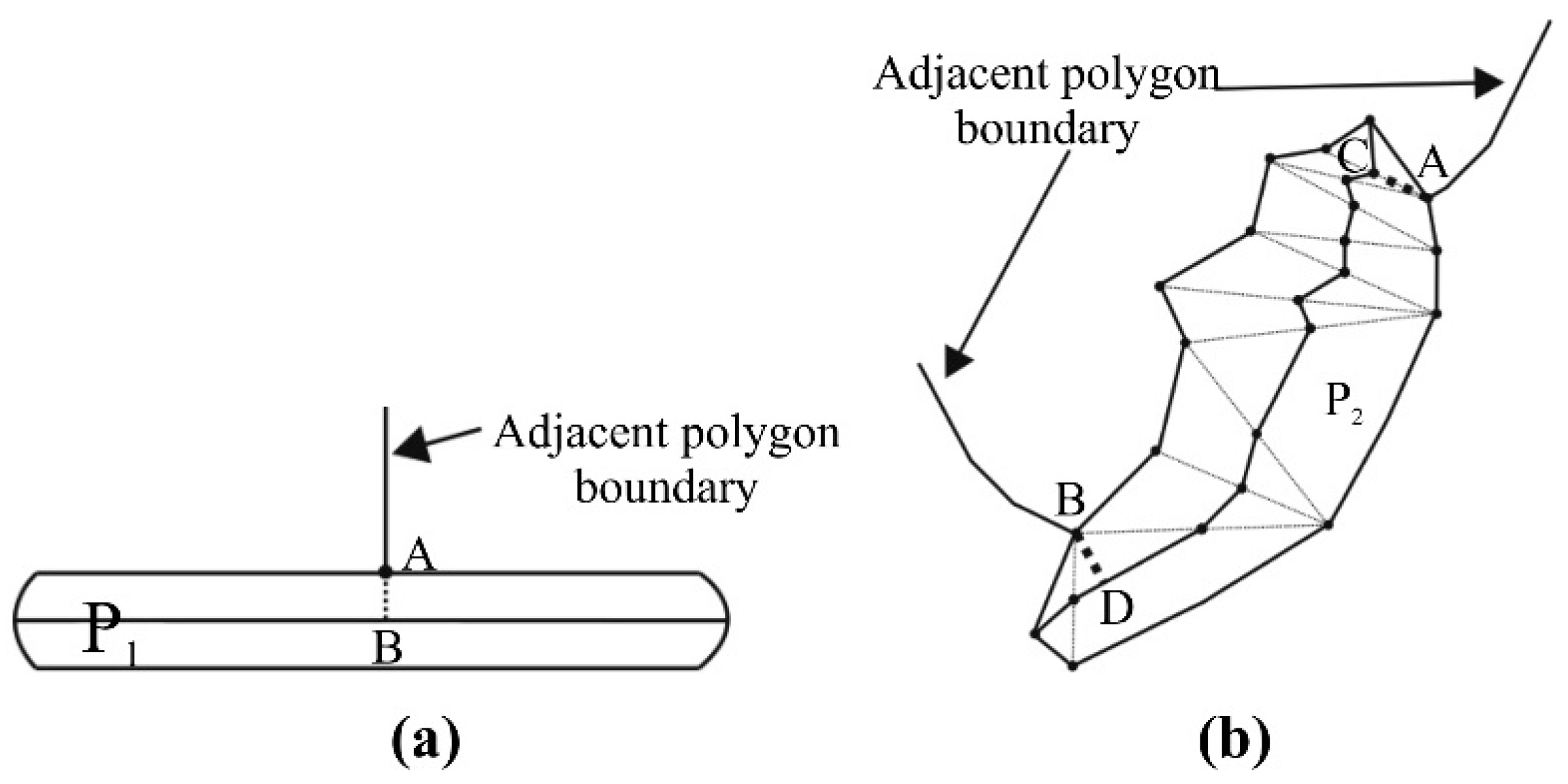
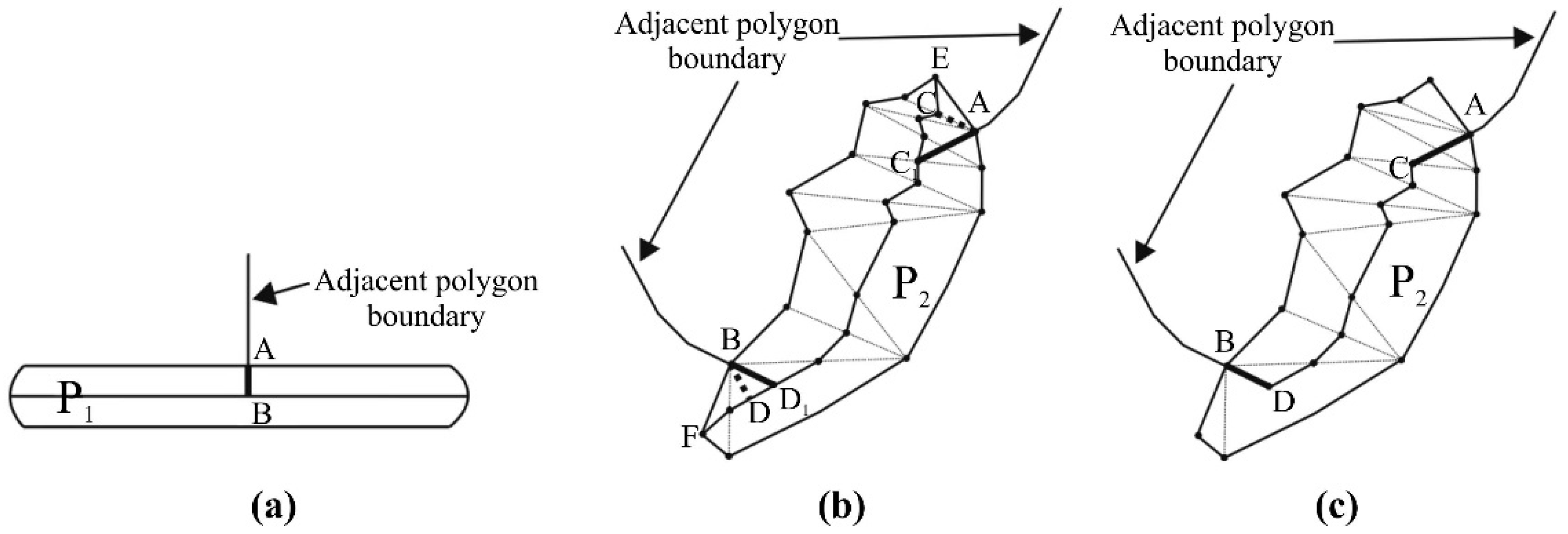
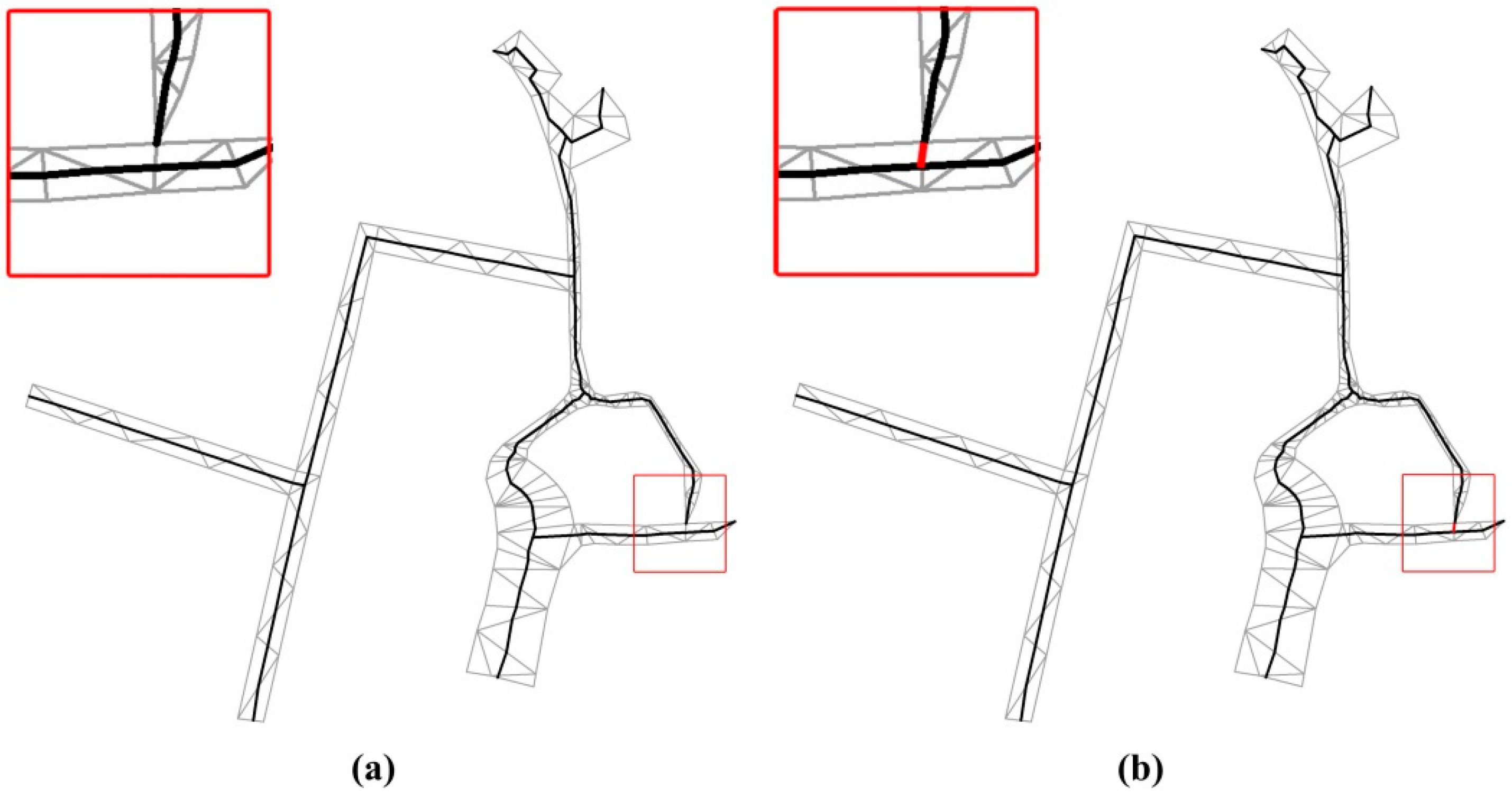
4.3.1. Topology Correction for Nodes with Degree 1

The boundary nodes which are associated with adjacent polygon only link one skeleton arc inside the polygon. As such, this is called a single node of the polygon, having a degree of 1 on the split line. As shown in Figure 11a, node A is a single node of polygonal P1. In Figure 11b, nodes A and B are single nodes of polygon P2. Because Delaunay triangulation is constructed based on boundary constraints, the intersection points of adjacent polygons and the boundary of the polygons to be divided (see A, B in Figure 11b) must be vertices in Delaunay triangles. However, these intersection points do not connect with the split lines because they are not on the main skeleton line. It is obvious that the split lines at the single nodes in these figures do not satisfy the aforementioned constraint imposed by the connecting nodes of adjacent polygon boundaries, thus the split lines need topology correction.

Figure 11. Topological relation constraints: (a) perpendicular to the boundary of adjacent polygon and (b) at an angle to the boundary of the adjacent polygon.

The most common method of split line topology correction is the closest point method [26] and the triangulation supplement method [27]. However, these two methods have less consideration for the extension nature of boundary lines. When the split line and the boundary line are perpendicular to each other, the effect of the new split line is better (see the arc segment AB in Figure 12a), and when the two lines have another angle relationship, the new split line is explicitly blunt (see the arc segment BD in Figure 12b). Thus, we propose a ‘reverse extension method’ as a complement to the closest point method. The basic idea is to determine the extension direction of the adjacent polygon boundary according to the positional relationship between the two adjacent boundary points near the patches. Then, the polygon boundary is extended along the opposite direction to intersect the split line of patches, and the boundary nodes are connected to the intersection points to get the split lines. As shown in Figure 12a, the adjacent polygon boundary is reversely extended from node A to node B, to obtain the new split line AB shown in Figure 12a. In Figure 12b, the adjacent polygon boundary composed of nodes A, B extends back to nodes C₁, D₁ in reverse, resulting in the new split lines AC₁, BD₁ in Figure 12b.

Figure 12. Split line topology correction method for nodes with degree 1: (a) closest point method, (b) reverse extension method and (c) dangling skeleton line removal.

Redundant skeleton line branches, such as C₁E and D₁F in Figure 12b, need to be deleted. The main operation for achieving this is the iterative deletion of dangling arcs in the skeleton topology, while retaining the new split line, until no more dangling arcs are found, and the final split line is obtained as shown in Figure 12c.

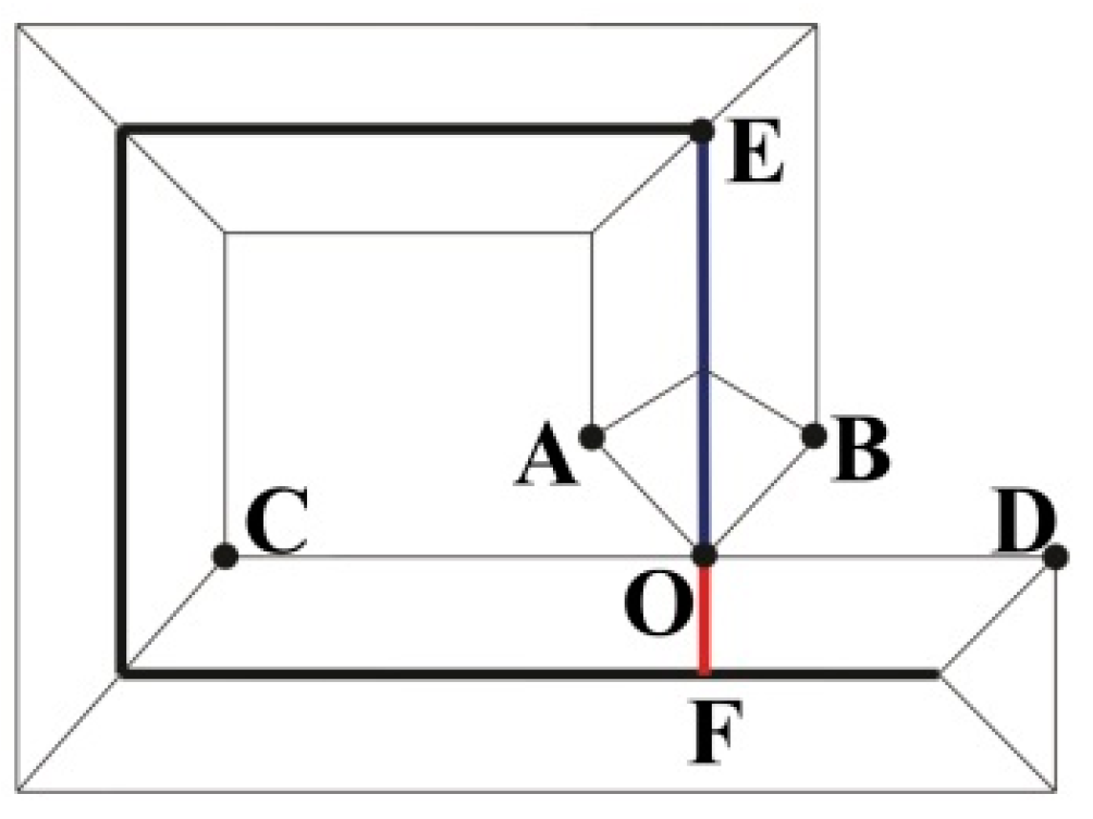
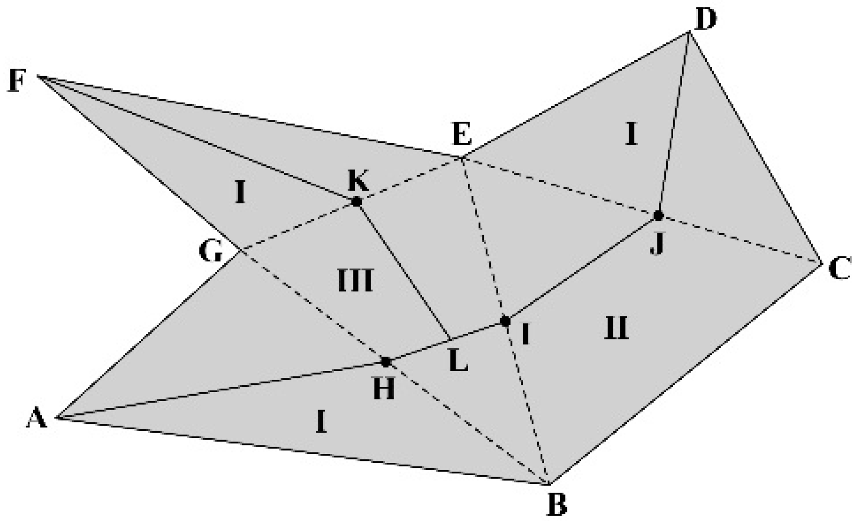
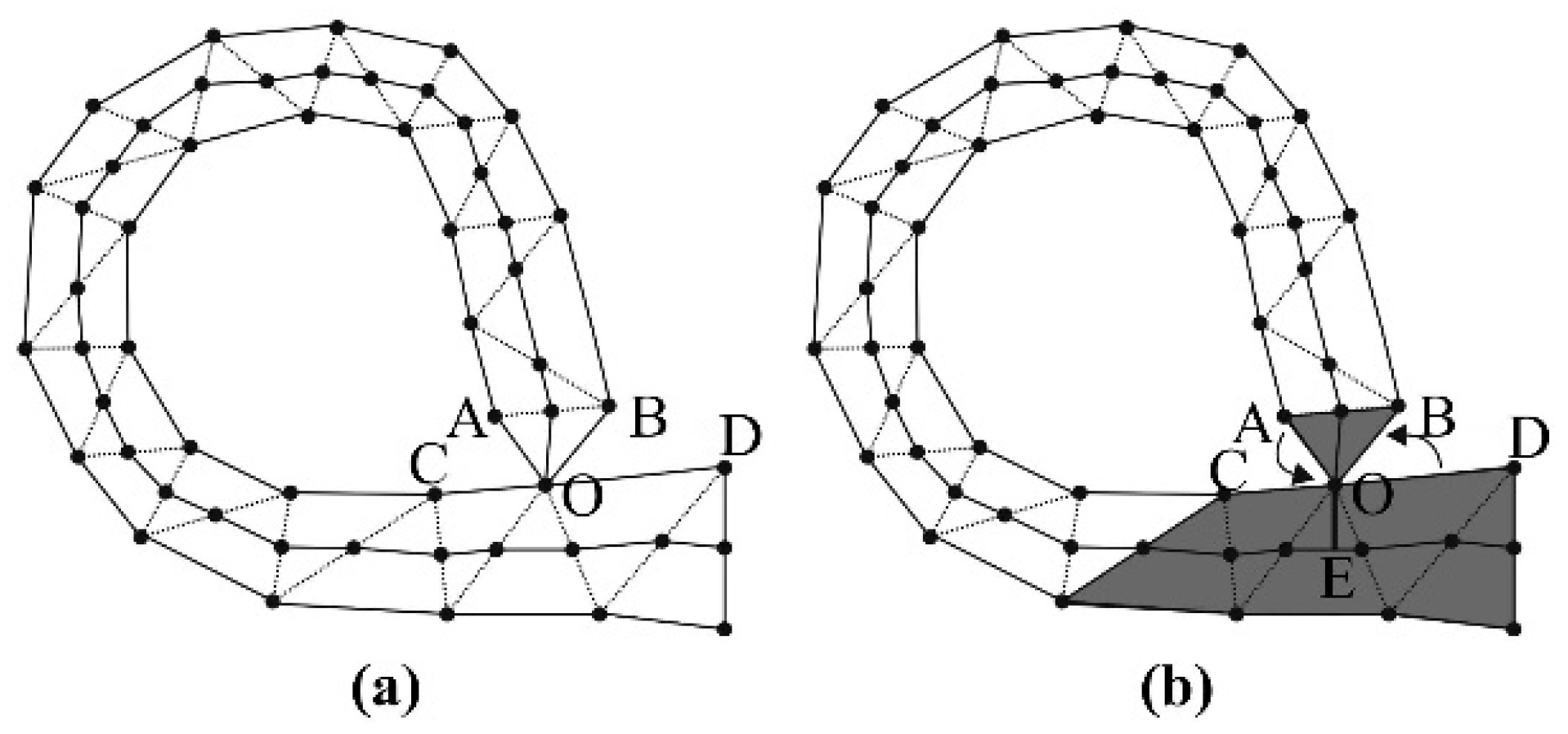
4.3.2. Topology Correction for Nodes with Degree 2

The topology of the original map is now established. By means of the topology relationship between <nodes, arcs> and <arcs, arcs>, a node with degree 2 on the split line can be identified. That is, when a node is associated with four connected arcs of the same polygon, the node has a degree of 4 on the original polygon and a degree of 2 on the split line inside the polygon. When using the traditional method to extract the split line at a node with a degree of 2, the extracted split line is inconsistent with the topology of the original polygon, as illustrated in Figure 13a. Hence, we propose a topology correction algorithm for a split line in a node with degree 2, the specific process for which is as follows:

Figure 13. Split line topology correction method for nodes with degree 2: (a) original polygon and (b) correction result.

Step 1: With point O as the origin, arrange the arc segments associated with O in a counter-clockwise (or clockwise) direction, and obtain the adjacent arc segments before and after each arc. For example, the adjacent arcs of OB are OA and OD.

Step 2: Select an arc segment randomly as initial arcs and judge the spatial relationship between the area formed by this arc and its adjacent arcs AdjArc (Area_{<Arc, AdjArc>}) and the original polygon.

(1)

If the area is inside the polygon and has a split line associated with point O, no action is taken.

(2)

If the area is inside the polygon and does not have a split line associated with point O, the closest point method is applied to correct it with the split line.

(3)

If the area is outside the polygon, no action is taken.

In Figure 13a, Area_{<OC, OD>} is inside the polygon and has no split line. It is then corrected with split line OE. Area_{<OA, OB>} is inside the polygon and has a split line. As such, no action is taken, as shown in Figure 13b.

5. Experiments and Results

Our improved jitter elimination and topology correction method for the split line of narrow and long patches was embedded within the WJ-III mapping workstation developed by the Chinese Academy of Surveying and Mapping. To verify the reliability of our method, we compared the processing result of the straight skeleton method with the method proposed in this paper on sample data; meanwhile, experiments conducted using actual data from China’s geographical conditions census in Guizhou province verified the superiority of our method.

5.1. Reliability Test and Analysis

In order to verify the reliability of our method, the split lines of the road data in Haunert and Sester [25] (Figure 14a) extracted using our method were compared with the split lines extracted using straight skeleton method (Figure 14b). A boundary-CDT was constructed for the narrow and long patches, and 1.6 mm was set to encrypt the boundary node. The threshold of the fitting length of the node in the junction was set to 0.4 mm, and the extraction results were obtained (Figure 14c).

Figure 14. Reliability test and analysis: (a) original data, (b) split line obtained with the proposal by Haunert and Sester [25] and (c) split line obtained using our method.

By observing the results in Figure 14b,c, the split line extracted from the original data according to our method is basically the same as the split line extracted by the method proposed by Haunert and Sester [25]. Both split lines suitably reflect the extension direction and spatial structure of the road network. The transition of the ‘T’- and ‘+’-type and its split lines in the rectangular box are smooth and there are no redundant hanging nodes. Thus, it correctly summarizes the main road network’s structure, confirming the reliability of our method when extracting split lines.

It is noteworthy that the road data given in Haunert and Sester [25] pertain to straight roads of a similar width and with a parallel extension on both sides. These regular polygons can be regarded as simple, and their split lines are relatively easy to extract. However, using the connection point reconstruction algorithm proposed by Haunert and Sester [25] will result in split line extraction errors when the data processed are the road or river data with several bends and irregular and complex junctions. Thus, we evaluated our method using polygons with irregular features, based on China’s geographical conditions census in Guizhou province. The results are described in the next subsection.

5.2. Superiority Test and Analysis

Actual data from China’s geographical conditions census in Guizhou province was used to verify the superiority of our method in preserving the spatial structure and topological relations of irregular and complex geomorphic objects. The spatial range of the data is 560 square kilometers, the original scale is 1:10,000, and the target scale for generalization is 1:100,000. The number of jitter elimination and topology correction completed in the experiment is shown in Table 1.

Table 1. Statistics of jitter elimination and topology correction in the experimental region.

	Jitter Elimination		Topology Correction		Total
	Spike Jitters	Jitters in Branch Junctions	Nodes with Degree 1	Nodes with Degree 2
Number	621	456	1513	3	2593
Proportion (%)	23.95	17.59	58.35	0.11	100

Three cases with actual data based on geographic conditions were selected to verify collapse operation, and one case was selected to verify split operation.

The characteristics of the region shown in Case 1 are as follows: Two branch junctions consisting of six branch roads—a, b, c, d, e, and f—are adjacent to each other, where a and b are in the same direction, and the direction of c and d is also the same, but the length of type II triangular internal skeleton line in the diagram is greater than 0.4 mm between the branch nodes, as shown in the rectangular box in Figure 15a. In this study, the structural features are reserved, and the two branch junctions are processed separately. According to the direction property, the split line is adjusted, as shown in Figure 15b. However, the distance between adjacent nodes in the rectangular frame of Figure 15b is less than 0.4 mm, so the split line is further optimized, as shown in Figure 15c. The dashed line in Figure 15c shows the split line extracted according to the method of Haunert and Sester [25]. A visual comparison clearly shows that the proposed method in this paper better preserves the structural characteristics of the area.

Figure 15. Case 1: Branch junctions with a consistent direction skeleton: (a) original skeleton lines, (b) split line extracted from skeleton lines considering direction features and (c) re-aggregation of the split lines in the branch junction.

The characteristics of the region shown in Case 2 are as follows: The directions of a, b, c, d, and e branch roads are not the same at the road junction shown in the rectangular box in Figure 16a. It is thus difficult to reconstruct the connection point based on branch skeleton line extension when fitting each branch to the same aggregation node, as shown in Figure 16b. Therefore, we connect the fitting node and the branch skeleton line to derive the split line by fitting all the nodes in this area to the geometric center, as shown in Figure 16c. It can be seen that our method appropriately adjusted the skeleton line in this case, although it also caused some jitters in the skeleton line in the region; this is an issue which we shall address in future research.

Figure 16. Case 2: Branch aggregation region with no consistent direction skeleton: (a) original skeleton lines, (b) split line extracted based on branch skeleton line extension and (c) split line extracted by fitting all the nodes to the geometric center.

The characteristics of the region shown in Case 3 are as follows: The ditches within the rectangular box in Figure 17a have a self-intersecting topological structure, and if the skeletal line is extracted directly, there will be no skeletal line at the node of degree 2. However, after correction for the skeleton line at the boundary, the split line was obtained, as shown in Figure 17b. It is clear that the adjusted skeleton line realized the topology correction at this site and effectively avoided topological errors.

Figure 17. Case 3: Self-intersection of narrow and long patches: (a) skeleton line extracted directly and (b) split line topology correction.

Case 4 is an example for split operation. A narrow road is surrounded by farmland, garden land, forest land and grassland, as shown in Figure 18a. Then the split line of this road was extracted according to the method proposed in this paper, as shown in Figure 18b. It can be seen that the splitting line at the boundary extends naturally. Figure 18c describes the result of the split operation. The result offers an appropriate representation for split operation of land-use thematic data with respect to topological and geometrical feature.

Figure 18. Case 4: Split operation for narrow and long patches: (a) original data, (b) split line of narrow and long patches and (c) result of split operation.

6. Discussion and Conclusions

Extracting the split line in narrow and long patches is an important and difficult problem for the generalization of land-use thematic data. Extracted split lines need to take into account natural and smooth geometric features and structural features that accord with visual perception and their actual topological features. By overcoming the shortcomings of the straight skeleton method, an improved method was proposed in this paper to extract split lines based on the constrained Delaunay triangulation. Our method removes jitters and topology correction for split lines accordingly in order to solve the problems of shape jitters and topological inconsistency along the skeleton line. Test results on sample data and actual geographic data show that our method not only appropriately extracts the split lines of long and narrow patches with regular shapes, but also well maintains the consistency of structural features and topological relations when dealing with the irregular and complex polygons.

As for our method, the densification step (D) plays an important role in avoiding the offset of the skeleton line at the boundary of the polygon, and when calculating the direction of each branch line in the branch convergence zone. If the threshold is too large, the skeletal line at the boundary of the polygon will appear partial. If the threshold value is too small, however, the filter of the type II triangle at the corner will be incomplete, leading to misjudgments of the direction of each branch skeleton line. Therefore, a method for selecting the threshold of the densification step must be sought for polygons with different geometrical characteristics and different geometries. We shall pursue this method in future research.

In addition, there have been some effective methods of solving the problem of topologically correct connection of a split line to the boundaries of adjacent polygons, we need to analyze the characteristics of these methods and our method in future work.

References

1. Van Oosterom, P. The GAP-tree, an approach to ‘on-the-fly’ map generalization of an area partitioning. In GIS and Generalization, Methodology and Practice; CRC Press: Boca Raton, FL, USA, 1995; pp. 120–132. [Google Scholar]
2. Beard, K.; Mackaness, W. Generalization operations and supporting structures. In Auto-Carto 10: Technical Papers of the 1991 ACSM-ASPRS Annual Convention; ACSM-ASPRS: Baltimore, ML, USA, 1991; Volume 6, pp. 29–45. [Google Scholar]
3. McMaster, R.B.; Shea, K.S. Generalization in Digital Cartography; Association of American Geographers: Washington, DC, USA, 1992. [Google Scholar]
4. Mitropoulos, V.; Xydia, A.; Nakos, B.; Vescoukis, V. The use of epsilon convex area for attributing bends along a cartographic line. In Proceedings of the 22nd International Cartographic Conference, La Corona, Spain, 9–16 July 2005. [Google Scholar]
5. Muller, J.C. Fractal and Automated Line Generalization. Cartogr. J. 1987, 24, 27–34. [Google Scholar] [CrossRef]
6. Lee, D.T. Medial axis transformation of a planar shape. IEEE Trans. Pattern Anal. Mach. Intell. 1982, 4, 363–369. [Google Scholar] [CrossRef] [PubMed]
7. Montanari, U. A method for obtaining skeletons using a quasi-Euclidean distance. J. ACM 1968, 15, 600–624. [Google Scholar] [CrossRef]
8. Ruas, A. Multiple paradigms for automating map generalization: Geometry, topology, hierarchical partitioning and local triangulation. ACSM/ASPRS Annu. Conv. Expos. 1995, 4, 68–69. [Google Scholar]
9. Ware, J.M.; Jones, C.B.; Bundy, G.L. A Triangulated Spatial Model for Cartographic Generalization of Areal Objects. In Advance in GIS Research II, Proceedings of the 7th International Symposium on Spatial Data Handling, Delft, The Netherlands, 12–16 August 1996; Kraak, M.J., Molenaar, M., Eds.; Taylor & Francis: London, UK, 1997; pp. 173–192. [Google Scholar]
10. Cao, T.; Edelsbrunner, H.; Tan, T. Proof of correctness of the digital Delaunay triangulation algorithm. Comput. Geom. Theory Appl. 2015, 48, 507–519. [Google Scholar] [CrossRef]
11. Sintunata, V.; Aoki, T. Skeleton extraction in cluttered image based on delaunay triangulation. In Proceedings of the 2016 IEEE International Symposium on Multimedia (ISM), San Jose, CA, USA, 11–13 December 2016; pp. 365–366. [Google Scholar]
12. Yu, W. Assessing the implications of the recent community opening policy on the street centrality in China: A GIS-based method and case study. Appl. Geogr. 2017, 89, 61–76. [Google Scholar] [CrossRef]
13. DeLucia, A.A.; Black, R.T. A Comprehensive Approach to Automatic Feature Generalization. In Proceedings of the 13th Conference of the International Cartographic Association, Morelia, Mexico, 12–21 October 1987; pp. 173–191. [Google Scholar]
14. Li, Z. Algorithmic Foundation of Multi-Scale Spatial Representation; CRC Press: Boca Raton, FL, USA, 2006. [Google Scholar]
15. Zou, J.J.; Yan, H. Skeletonization of ribbon-like shapes based on regularity and singularity analyses. IEEE Trans. Syst. Man Cybern. Part B 2001, 31, 401–407. [Google Scholar]
16. Morrison, P.; Zou, J.J. Triangle refinement in a constrained Delaunay triangulation skeleton. Pattern Recognit. 2007, 40, 2754–2765. [Google Scholar] [CrossRef]
17. Penninga, F.; Verbree, E.; Quak, W.; van Oosterom, P. Construction of the Planar Partition Postal Code Map Based on Cadastral Registration. GeoInformatica 2005, 9, 181–204. [Google Scholar] [CrossRef]
18. Uitermark, H.; Vogels, A.; Van Oosterom, P. Semantic and Geometric Aspects of Integrating Road Networks. In Proceedings of the Second International Conference on Interoperating Geographic Information Systems (INTEROP’99), Zürich, Switzerland, 10–12 March 1999; Vþkovski, A., Brassel, K.E., Schek, H.-J., Eds.; Springer: Berlin/Heidelberg, Germany, 1999; pp. 177–188. [Google Scholar]
19. Jones, C.B.; Bundy, G.L.; Ware, M.J. Map Generalization with a Triangulated Data Structure. Cartogr. Geogr. Inf. Syst. 1995, 22, 317–331. [Google Scholar]
20. Gao, P.; Minami, M.M. Raster-to-vector Conversion: A Trend Line Intersection Approach to Junction Enhancement. In Proceedings of the 11th International Symposium on Computer-Assisted Cartography, Minneapolis, MN, USA, 30 October–1 November 1993; pp. 297–304. [Google Scholar]
21. Aichholzer, O.; Aurenhammer, F.; Alberts, D.; Gärtner, B. A Novel Type of Skeleton for Polygons. J. Univers. Comput. Sci. 1996, 1, 752–761. [Google Scholar]
22. Das, G.K.; Mukhopadhyay, A.; Nandy, S.C.; Patil, S.; Rao, S.V. Computing the straight skeleton of a monotone polygon in O(nlogn) time. In Proceedings of the 22nd Annual Canadian Conference on Computational Geometry, Winnipeg, MB, Canada, 9–11 August 2010; pp. 207–210. [Google Scholar]
23. Eppstein, D.; Erickson, J. Raising roofs, crashing cycles, and playing pool: Applications of a data structure for finding pairwise interactions. Discret. Comput. Geom. 1999, 22, 569–592. [Google Scholar] [CrossRef]
24. Haunert, J.H.; Sester, M. Using the straight skeleton for generalization in a multiple representation environment. In Proceedings of the 8th ICA Workshop on Generalization and Multiple Representation, Leicester, UK, 20–21 August 2004. [Google Scholar]
25. Haunert, J.H.; Sester, M. Area collapse and road centerlines based on straight skeletons. GeoInformatica 2008, 12, 169–191. [Google Scholar] [CrossRef]
26. Ai, T.; Yang, F.; Li, J. Land-use Data Generalization for the Database Construction of the Second Land Resource Survey. Geomat. Inf. Sci. Wuhan Univ. 2010, 35, 887–891. (In Chinese) [Google Scholar]
27. Meijers, M.; Savino, S.; Van Oosterom, P. SPLITAREA: An algorithm for weighted splitting of faces in the context of a planar partition. Int. J. Geogr. Inf. Sci. 2016, 30, 1522–1551. [Google Scholar] [CrossRef]
Article Metrics
Citations
Article Access Statistics
Multiple requests from the same IP address are counted as one view.