Continuous Scale Transformations of Linear Features Using Simulated Annealing-Based Morphing

Abstract

This paper presents a new method for use in performing continuous scale transformations of linear features using Simulated Annealing-Based Morphing (SABM). This study addresses two key problems in the continuous generalization of linear features by morphing, specifically the detection of characteristic points and correspondence matching. First, an algorithm that performs robust detection of characteristic points is developed that is based on the Constrained Delaunay Triangulation (CDT) model. Then, an optimal problem is defined and solved to associate the characteristic points between a coarser representation and a finer representation. The algorithm decomposes the input shapes into several pairs of corresponding segments and uses the simulated annealing algorithm to find the optimal matching. Simple straight-line trajectories are used to define the movements between corresponding points. The experimental results show that the SABM method can be used for continuous generalization and generates smooth, natural and visually pleasing linear features with gradient effects. In contrast to linear interpolation, the SABM method uses the simulated annealing technique to optimize the correspondence between characteristic points. Moreover, it avoids interior distortions within intermediate shapes and preserves the geographical characteristics of the input shapes.

1. Introduction

With the development of web mapping and big geo-data, there have been significant changes in the goals and methods of map generalization. Th goals of map generalization are to settle the problem of embedding spatial data covering a large region into a small space and to discover geospatial knowledge by data abstraction [1,2,3,4]. The mode of map services should support interactive zooming in and out to arbitrary scales [5]. Traditional Multi-Scale Databases (MSDBs) do not meet the demands of users for arbitrary scaling [6]. To overcome these deficiencies, some new methods have emerged, such as continuous generalization, on-the-fly generalization and on-demand mapping [7,8,9].This study explores the problem of the continuous generalization of linear map features by shape morphing.

Continuous generalization denotes the use of various generalization techniques in real time to generate geographic information at arbitrary scales with smooth and continuous changes. This process creates temporary, generalized datasets exclusively for visualization; however, these datasets are not stored or used for other purposes. There are three solutions for online continuous generalization, specifically the traditional cartographic generalization algorithm-based solution, the LOD-based solution and the shape morphing-based solution. The first solution implements continuous generalization by selecting and transforming the traditional cartographic generalization algorithm for data processing in a network environment. For example, Sester and Brenner [7] defined a set of elementary generalization operations (EGOs) and used them to perform continuous generalization of building areas on small mobile devices. The LOD-based solution relies on the accumulation of change to construct a multiscale entity model [10,11]. This model considers the spatial representation from one scale to another as the accumulation of a set of changes. The difference between two consecutive representations is recorded in a linear order, and the target representation is achieved through the gradual addition or subtraction of “change patches”. The third solution achieves continuous generalization based on shape morphing by obtaining a map representation at a meaningful intermediate scale and interpolating between the two anchor scales [12,13,14,15,16]. The interpolated result is coarser than that at the larger scale and finer than that at the smaller scale, thereby reflecting the fusion of the two basic scales.

Shape morphing is an important technique in computer graphics and computer vision [17]. In general, morphing can be defined as a gradual (i.e., over time) and smooth transformation of one key shape into another [18]. Previous studies have mainly focused on two aspects, i.e., finding meaningful correspondences between the characteristics of two key shapes and producing smooth interpolated shapes according to “trajectories” along which the characteristics change from one key shape to another. Generally, the process of characteristic correspondence is to detect the characteristic points and to establish the correspondence between the geometric features of the source and target shapes. In the field of computer graphics, the relationship of correspondence is usually computed based on physical energy minimization or the geometric similarity of the shapes [19,20,21]. The use of path interpolation in morphing ensures that, as the intermediate shapes change gradually along a specified trajectory, the boundaries of the intermediates display no shrinkage and the interiors are not distorted. The simplest method is linear interpolation, which is only suitable for simple shapes. Sederberg et al. [22] proposed an intrinsic interpolation method that avoids shrinkage by interpolating both the edge lengths and the vertex angles of two input shapes. Moreover, the as-rigid-as-possible interpolation method has been described that improves the effectiveness of boundary interpolation by rigid motion and compatible triangulations [23,24].

Generally, in cartography and other fields, the process of characteristic point matching plays an important role in morphing. Unreasonable matching may result directly in poor warping results. Simple matching methods based on local geometric properties, such as vertex angles, edge lengths or triangle areas, are insufficient to describe and match the geographical properties hidden within geometric shapes [3]. Proper characteristic matching must consider the geometric, topological and semantic similarities of geographical features. Therefore, matching is a global process and requires optimization to obtain reasonable results. In this study, simulated annealing, a global optimization algorithm [25], is applied to carry out characteristic matching and shape interpolation. Finally, the continuous generalization of linear features is carried out.

The rest of paper is organized as follows. Section 2 investigates the continuous scale transformation model of linear feature using a simulated annealing-based morphing technique. Experiments involving simulated data and different real linear features are given in Section 3. Section 4 presents the conclusions of this study, together with suggestions for future improvements.

2. Methodology

The concept model of morphing can be expressed as ${\mathrm{R}}_{\mathrm{s}}=\mathsf{\pi }\left(\mathsf{\alpha },\mathsf{\beta },\mathrm{s}\right)$, in which $\mathsf{\pi }$ is a continuous and monotonic interpolating function of $\mathrm{s}$; $\mathrm{s}$ is a normalized parameter related to the scale; α is the linear feature of the source, which has a large built-in scale; β is the linear feature of the target, which has a small built-in scale; and ${\mathrm{R}}_{\mathrm{s}}$ is the interpolation shape, which ranges from $\mathsf{\alpha }\mathrm{to}\mathsf{\beta }$. The whole process consists of four major steps, specifically collecting user inputs, extraction of characteristic points, assessment of the correspondence between characteristic points and path interpolation. Because β is generalized from α, all of the characteristic points on β have corresponding points on α, but not vice versa. The relationship between $\mathrm{s}$ and the scale is as follows:

$$\mathrm{s}=\frac{\frac{1}{{\mathrm{T}}_{\mathrm{Mid}}}-\frac{1}{{\mathrm{T}}_{\mathrm{a}}}}{\frac{1}{{\mathrm{T}}_{\mathrm{b}}}-\frac{1}{{\mathrm{T}}_{\mathrm{a}}}}$$

(1)

where ${\mathrm{T}}_{\mathrm{a}}$, ${\mathrm{T}}_{\mathrm{b}}\mathrm{and}{\mathrm{T}}_{\mathrm{Mid}}$ are the scales of $\mathsf{\alpha },\mathsf{\beta }\mathrm{and}{\mathrm{R}}_{\mathrm{s}}$, respectively.

Assume that polyline α is a curve specified by a sequence of points $\mathrm{SP}:\{{\mathrm{a}}_1,{\mathrm{a}}_2\dots {\mathrm{a}}_{\mathrm{m}}\}$ that are called its vertices, polyline β is a curve specified by a sequence of points $\mathrm{TP}:\{{\mathrm{b}}_1,{\mathrm{b}}_2\dots {\mathrm{b}}_{\mathrm{n}}\}$ that are called its vertices, the number of characteristic points on β is k, and their indexes in the coordinate string are $\mathrm{TK}:\{{\mathrm{g}}_1,{\mathrm{g}}_2\dots {\mathrm{g}}_{\mathrm{k}}\}$. Then, the characteristic point series of β can be determined as $\mathrm{TS}:\{{\mathrm{b}}_{{\mathrm{g}}_1},{\mathrm{b}}_{{\mathrm{g}}_2}\dots {\mathrm{b}}_{{\mathrm{g}}_{\mathrm{k}}}\}$, where ${\mathrm{b}}_{{\mathrm{g}}_{\mathrm{j}}}\in \mathrm{TP}\mathrm{and}{\mathrm{g}}_{\mathrm{j}}\in \mathrm{TK}$. The extraction of characteristic points is introduced in Section 2.1., and the correspondence of characteristic points is introduced in Section 2.2. Path interpolation is presented in Section 2.3.

2.1. Characteristic Point Extraction

A CDT-based method is adopted to detect the characteristic points of polylines. The results of this method divide polylines into groups of symmetrical bends. The process of characteristic point extraction is shown in Algorithm 1.

Algorithm 1 Characteristic Point Extraction

Input: points on β $\mathbf{TP}:\{{\mathbf{b}}_1,{\mathbf{b}}_2\dots {\mathbf{b}}_{\mathbf{n}}\}$.  Output: characteristic points of β.  For polyline β at small scale do   1 Construction of CDT   2 Classification of triangles   3 Extraction of characteristic points   4 Elimination of pseudo-characteristic points   5 Supplement with start and end points  End

All the points and segments of β are taken into account in constructing the CDT, in which the segments play the role of constrained edges. The triangles in the network are classified into three types based on the number of unconstrained edges of each triangle. Triangles with one unconstrained edge are defined as type I triangles, those with two unconstrained edges are defined as type II triangles, and those with three unconstrained edges are defined as type III triangles. In Figure 1a, triangle C belongs to type I, triangle B belongs to type II, and triangle A belongs to type III. The intersection points of the two constrained edges of each type I triangle are extracted as characteristic points. In Figure 1a, the arrow shows the direction of the polyline, and the red points are raw extracted characteristic points, in which the square points are formed by external bends and the circle points are formed by internal bends.

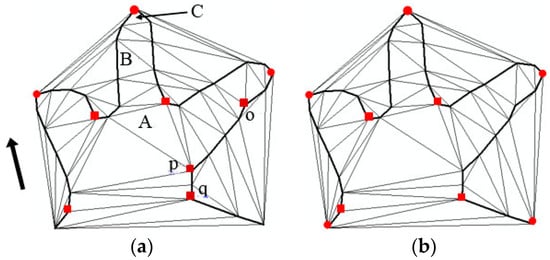
Figure 1. The extraction of characteristic points. (a) Raw characteristic points with pseudo-characteristic points. (b) Final characteristic points after excluding the pseudo-characteristic points and supplementing with the endpoints.

The method of extracting characteristic points directly based on triangulation has a drawback in that it is sensitive to coordinate tremble and the existence of pseudo-characteristic points. In Figure 1a, the characteristic points o, p and q are generated by coordinate tremble. To improve the quality of the characteristic points, the characteristic points that satisfy the following two criteria are eliminated. If a type III triangle is directly adjacent to a type I triangle, then the characteristic point on the latter will be deleted (e.g., point o in Figure 1a). In addition, if one type III triangle has two directly adjacent type I triangles, the characteristic point on the type I triangle with a small area will be deleted (e.g., point p in Figure 1a). After the exclusion of the pseudo-characteristic points, circle and square characteristic points appear alternately along the polyline. Lastly, the start and end points of β are added to the set of its characteristic points. The final characteristic points are shown in Figure 1b.

2.2. Characteristic Point Correspondence Using the Simulated Annealing Algorithm

For each characteristic point in $\mathrm{TS}$, a corresponding point in $\mathrm{SP}$ can be found. The result of correspondence establishes a relationship between $\mathrm{TS}$ and $\mathrm{SP}\mathsf{\gamma }:\mathrm{TS}\to \mathrm{SP}$. Because the cardinality of $\mathrm{SP}$ is greater than that of $\mathrm{TS}$, there are many kinds of possible corresponding relationships between $\mathrm{TS}$ and $\mathrm{SP}$. Which corresponding relationship is the best? This is an optimization problem. First, an objective function is built that evaluates the rationality of each correspondence $\mathsf{\gamma }$. A metric function $\mathrm{d}\left(\mathrm{TS},\mathrm{SP},\mathsf{\gamma }\right)$ is defined to evaluate the differences between two series of segments. Obviously, smaller values of d indicate a more reasonable correspondence. Our purpose is to find a correspondence $\mathsf{\gamma }$ that causes the metric function $\mathrm{d}\left(\mathrm{TS},\mathrm{SP},\mathsf{\gamma }\right)$ to achieve its minimum value. The SA algorithm is employed to identify the optimal correspondence. SA is a random-search technique that exploits an analogy between the way in which metals cool and freeze into a minimum-energy crystalline structure (the annealing process) and the search for a minimum in a more general system [25,26]. As a generic probabilistic meta-heuristic for the global optimization problem of locating a good approximation to the global optimum of a given function, it is used to identify the optimum matching with the minimum possible energy based on the objective function d.

The algorithm process of identifying the correspondence of characteristic points by simulated annealing is shown in Algorithm 2. First, an arbitrary initial matching state ${\mathsf{\gamma }}_0$ is generated using the Monte Carlo method. For each characteristic point in $\mathrm{TS}$, a random point is selected from its candidate set as the corresponding point to generate the initial matching state ${\mathsf{\gamma }}_0:\mathrm{TS}\to \mathrm{SP}$. Then, the SA algorithm obtains the global optimal result through slow cooling. In each cooling step, the SA heuristic considers some neighboring state ${\mathsf{\gamma }}^{\prime }$ of the current state $\mathsf{\gamma }$ and decides probabilistically whether to move to state ${\mathsf{\gamma }}^{\prime }$ or to remain in state $\mathsf{\gamma }$. These probabilities ultimately lead the model to move to a lower energy state. Typically, this step is repeated until the model reaches a state that is good enough for the application, or until a predetermined computational budget has been exhausted. The efficiency of the algorithm and the quality of the matching results depend on four factors, namely the objective function, the search space, the acceptance probabilities and the annealing schedule.

2.2.1. Objective Function

Here, the purpose of the objective function is to evaluate the differences in curves. There are various types of metrics for evaluating the differences between two curves, such as distance, length, orientation, and shape. In the context of map generalization, these metrics may not work well. For example, if the target polyline is generated from the source polyline by bend deletion, then the length may become shorter, and the orientation may rotate by a certain amount. Here, the degree of overlap between the buffer areas of pairs of features are used as a metric to evaluate the similarity of features. Obviously, if two homologous geographic linear features are similar, then the degree of overlap of their buffer areas will be large, and vice versa. The Hausdorff distance between the two curves is used as the radius of the buffer function. This method ensures that the buffer function can adaptively adjust the radius to ensure that the overlap area is neither too broad nor too narrow and that the two buffers have a sufficient degree of overlap. Now, the differences in the two segments σ and τ can be defined as:

$$\mathrm{d}(\mathsf{\sigma },\mathsf{\tau })=1-\min \{\frac{{\mathrm{B}}_{\mathsf{\sigma }}{\displaystyle \cap }{\mathrm{B}}_{\mathsf{\tau }}}{{\mathrm{B}}_{\mathsf{\sigma }}},\frac{{\mathrm{B}}_{\mathsf{\sigma }}{\displaystyle \cap }{\mathrm{B}}_{\mathsf{\tau }}}{{\mathrm{B}}_{\mathsf{\tau }}}\}$$

(2)

Here, $\mathsf{\sigma }$ is a segment belonging to $\mathsf{\alpha }$, $\mathsf{\tau }$ is a segment belonging to $\mathsf{\beta },\mathrm{and}\mathrm{B}$ is the buffer function. The radii ${\mathrm{B}}_{\mathsf{\sigma }}$ and ${\mathrm{B}}_{\mathsf{\tau }}$ are defined by the Hausdorff distances of $\mathsf{\sigma }$ and $\mathsf{\tau }$. Then, for one certain correspondence $\mathsf{\gamma }$, the global difference can be defined as the sum of the local differences of all of the curves.

$$\mathrm{d}\left(\mathsf{\alpha },\mathsf{\beta },\mathsf{\gamma }\right)={\displaystyle \sum _{\mathrm{i}=1}^{\mathrm{k}-1}}{\mathrm{d}}_{\mathrm{i}}\left(\mathsf{\sigma },\mathsf{\tau }\right)$$

(3)

Here, k is the number of characteristic points, and k − 1 is the number of segments.

Algorithm 2 Correspondence of Characteristic Points by SA

Input: Initial matching state ${\mathit{\gamma }}_{\mathbf{0}}:\mathit{T}\mathit{S}\to \mathit{S}\mathit{P}$, initial temperature T0, annealing speed w.  Output: Optimum correspondence for $\mathit{T}\mathit{S}$ and $\mathit{S}\mathit{P}$.

Evaluate initial matching state

If (initial state = solution) then

Final state $\leftarrow$ initial state

Else

Current state $\leftarrow$ initial state

Initialize T0 according to annealing schedule

Do

Select candidate corresponding point that has not yet been applied to the current state

Apply candidate corresponding point to produce a new state

Evaluate new state

Compute $\Delta d$

If (new state is better than current state) then

Current state $\leftarrow$ new state

Else

P $\leftarrow e^{-\Delta d/T}$

Generate random number R between 0 and 1

If (R<P) then

Current state $\leftarrow$ new state

Endif

Endif

Revise T according to annealing schedule

Until (current state = solution ) or (no new candidate corresponding points left to apply)

Final state $\leftarrow$ current state

Endif

2.2.2. Search Space

A state $\mathsf{\gamma }$ is a matching between the characteristic points of $\mathrm{TS}$ and the coordinate points of $\mathrm{SP}\mathsf{\gamma }:\mathrm{TS}\to \mathrm{SP}$. The neighbors of a state are new states that are produced by altering a given state in well-defined ways. Based on state $\mathsf{\gamma }$, if the point that corresponds to a characteristic point ${\mathrm{b}}_{\mathrm{i}}$ is changed, say from ${\mathrm{a}}_{\mathrm{j}}$ to ${\mathrm{a}}_{\mathrm{k}}$, we obtain a neighbor ${\mathsf{\gamma }}^{\prime }$.

To improve the algorithm’s efficiency, a candidate corresponding set is defined for each characteristic point in $\mathrm{TS}$ to limit the search space. As two different representations of the same geographical entity, the corresponding points on $\mathsf{\alpha }$ and $\mathsf{\beta }$ have similar spatial locations. This property can be used to narrow the search space of the characteristic points. For each characteristic point in $\mathrm{TS}$, the Euclidean distances between it and all vertexes of α are calculated, and the vertex with the shortest distance as an anchoring point is selected. All the anchoring points divide α into $\mathrm{k}-1$ segments. If a₁, a₂ and a₃ are three neighboring anchoring points, the segment between a₁ and a₂ is defined as the preceding segment of a_2, and the segment between a₂ and a₃ is defined as the following segment of a₂. The half vertexes of the two neighboring segments near the current anchoring point are selected as the candidate corresponding set of the related characteristic point. Using this method, the matching process is first solved in a broad region of the search space containing good solutions before shifting to low-energy regions. The solution space becomes narrower and narrower, and finally, the downhill movement according to the steepest descent heuristic is used.

2.2.3. Acceptance Probabilities

As a meta-heuristic method, SA uses the neighbors of a state as a way to explore solution spaces, and although it prefers better neighbors, it also accepts worse or equally acceptable neighbors to avoid getting stuck in local optima. However, in cases where the new state is worse than or equal to the current state, simulated annealing has some probability of accepting the new state. The probability of making the transition from the current state $\mathsf{\gamma }$ to a candidate new state ${\mathsf{\gamma }}^{\prime }$ is specified by an acceptance probability function $\mathrm{P}\left(\mathsf{\gamma },{\mathsf{\gamma }}^{\prime },\mathrm{T}\right)$, which is defined as

$$\mathrm{P}\left(\mathsf{\gamma },{\mathsf{\gamma }}^{\prime },\mathrm{T}\right)={\mathrm{e}}^{-\Delta \mathrm{d}/\mathrm{T}}$$

(4)

$\Delta \mathrm{d}$ represents the “badness” of the new state, i.e., the amount by which the evaluation function is worsened; $\mathrm{d}\left(\mathrm{TS},\mathrm{SS},{\mathsf{\gamma }}_{\mathrm{i}}\right)-\mathrm{d}\left(\mathrm{TS},\mathrm{SS},{\mathsf{\gamma }}_0\right)$. $\mathrm{P}\left(\mathsf{\gamma },{\mathsf{\gamma }}^{\prime },\mathrm{T}\right)$ decreases exponentially as $\Delta \mathrm{d}$ increases (i.e., a slightly worse new state is more likely to be accepted than a much worse one). T, which is called the temperature, decreases over time according to an annealing schedule. At higher values of T, “bad” moves are more likely to be accepted. In practice, the probability P is usually tested against a random number R(0 $\le$ R $\le$ 1). A value of R $<$ P results in the new state being accepted.

2.2.4. Annealing Schedule

The initial choice of T and the rate at which it decreases has an effect on how well the algorithm performs [25]. When ${\mathrm{T}}_0$ is set to a larger value, the evolution of $\mathsf{\gamma }$ will only be sensitive to large variations in d. Under such conditions, the annealing process will be slow and will take a long time, but the algorithm is more likely to obtain the optimal matching results. In contrast, small values of ${\mathrm{T}}_0$ will result in sensitive evolution of $\mathsf{\gamma }$ given even small variations in d. Meanwhile, the annealing process will be quick and will take a small amount of time; however, the algorithm may miss the optimal matching results. Generally, the slower the rate of change, the better the result. However, the processing overhead associated with the algorithm increases as the rate of change of T becomes more gradual. In practice, a suitable annealing schedule is usually decided upon after some preliminary experimentation.

2.3. Path Interpolation

Piecewise linear interpolation is used to carry out the path interpolation. For each pair of segments, the number of vertexes is made to be equal by adding points to the middle position of the two neighboring vertexes with the biggest Euclidean distance one by one. Simple straight-line trajectories are then used to define the paths between corresponding points.

3. Case Study

The algorithms are evaluated using pairs of simulated data and two different types of real linear geographic features, specifically contour at scales of 1:10,000 and 1:50,000 and river network features at scales of 1:100,000 and 1:250,000. The simulated data covers the basic operations of map generalization for line features, which include vertex deletion, bend deletion, bend exaggeration and bend typification. Only those morphing transformations that take into account the basic generalization operations can be used for continuous scale transformations of map data. These real linear geographic features were obtained from the national fundamental geographic information system of China. They represent typical linear features found on maps and have a high degree of complexity. Here, they are used mainly to test the efficiency and availability of the algorithm. All of the experiments were performed on a DELL OptiPlex 3020 MT PC with an Intel^® Core^TM i5-4590 CPU and 8 GB of main memory running Microsoft Windows 7. The algorithms used to detect the characteristic points, determine the correspondence and perform the shape interpolation were implemented in C⁺⁺ and compiled with VS2012.

3.1. Simulation Experiments and Analysis

The simulated data are two representations on different scales. Figure 2a is the finer representation at a large scale (1:10,000) that has 119 vertexes and contains rich detail. Figure 2b is the related coarse representation at a small scale (1:50,000), which includes fewer details. Figure 3 shows the overlap of the two different representations. From this figure, it can be seen that the coarser representation is generalized from the finer one by four types of classic map generalization operations: the area of A being generalized by vertex deletion, the area of B being generalized by bend deletion, the area of C being generalized by bend exaggeration and the area of D being generalized by bend typification in order to reduce a series of three bends to two bends.

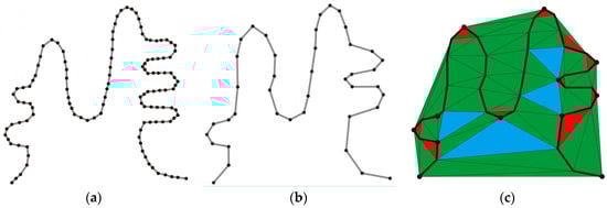
Figure 2. The experimental data with different levels of details and the characteristic point extraction from coarse representation of small scale. (a) Large-scale representation (1:10,000). (b) Small-scale representation (1:50,000). (c) Detection of characteristic points.

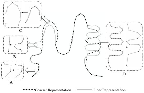
Figure 3. Applying the typical generalization operations to linear features.

The extraction of characteristic points was conducted using algorithm 1, which is described in Section 2.1. In Figure 2c, the different types of triangles are filled using three colors. Red is used for type II, green is used for type I, and blue is used for type III. After the elimination of pseudo-characteristic points and supplementing with the start and end points, the final 13 characteristic points are marked with small black circles in Figure 2c.

According to the rules of the search space presented in Section 2.2.2, the matching candidate sets of each characteristic point are extracted, and the results are listed in Table 1. The start and end points each have one and only one candidate. Each of the internal characteristic points has multiple candidates, which will be filtered using the SA-based correspondence algorithm.

Table 1. The characteristic points in Figure 2b and the related matching candidates (TS: characteristic points; CP: candidate points).

TS	CP	TS	CP	TS	CP	TS	CP
${\mathrm{b}}_1$	$\{{\mathrm{a}}_1\}$	${\mathrm{b}}_{12}$	$\{{\mathrm{a}}_{23},\dots ,{\mathrm{a}}_{35}\}$	${\mathrm{b}}_{30}$	$\{{\mathrm{a}}_{68},\dots ,{\mathrm{a}}_{75}\}$	${\mathrm{b}}_{41}$	$\{{\mathrm{a}}_{119}\}$
${\mathrm{b}}_3$	$\{{\mathrm{a}}_4,\dots ,{\mathrm{a}}_8\}$	${\mathrm{b}}_{18}$	$\{{\mathrm{a}}_{36},\dots ,{\mathrm{a}}_{49}\}$	${\mathrm{b}}_{33}$	$\{{\mathrm{a}}_{76},\dots ,{\mathrm{a}}_{83}\}$
${\mathrm{b}}_5$	$\{{\mathrm{a}}_9,\dots ,{\mathrm{a}}_{12}\}$	${\mathrm{b}}_{25}$	$\{{\mathrm{a}}_{50},\dots ,{\mathrm{a}}_{60}\}$	${\mathrm{b}}_{36}$	$\{{\mathrm{a}}_{84},\dots ,{\mathrm{a}}_{97}\}$
${\mathrm{b}}_7$	$\{{\mathrm{a}}_{13},\dots ,{\mathrm{a}}_{22}\}$	${\mathrm{b}}_{28}$	$\{{\mathrm{a}}_{61},\dots ,{\mathrm{a}}_{67}\}$	${\mathrm{b}}_{38}$	$\{{\mathrm{a}}_{98},\dots ,{\mathrm{a}}_{113}\}$

In this paper, a linear annealing schedule that is described by the function ${\mathrm{t}}_{\mathrm{new}}={\mathrm{w}\ast \mathrm{t}}_{\mathrm{old}}$ is used. Here, w controls the annealing speed, and this parameter decreases from 0.9 to 0.3. The initial temperature ${\mathrm{T}}_0$ decreases from 13 to 3. The results of the characteristic corresponding links with different annealing speeds w and initial temperatures ${\mathrm{T}}_0$ are shown in Figure 4. It can be seen that the linear annealing schedule is the key factor influencing the matching results when the initial temperature is sufficiently high for the annealing speed. The results of characteristic point correspondence have been quantitatively evaluated by C_tnl [13]. Defining a function e: [0,1] → E, where e(u) = g(u) − f(u) and u $\in$ [0,1], the length |E| of the linear feature E is the value of C_tnl [14]. A smaller C_tnl value indicates more accurate corresponding points. The run times and translation costs C_tnl that would result from different annealing rates w and initial temperatures ${\mathrm{T}}_0$ are shown in Table 2 and Figure 5.

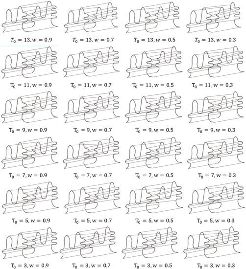
Figure 4. Characteristic corresponding links for different annealing speeds and initial temperatures.

Table 2. The running time (in milliseconds) and C_tnl (in meters) with different annealing speeds and initial temperatures.

	w = 0.9		w = 0.7		w = 0.5		w = 0.3
	Running Time	${\mathbf{C}}_{\mathbf{tnl}}$	Running Time	${\mathbf{C}}_{\mathbf{tnl}}$	Running Time	${\mathbf{C}}_{\mathbf{tnl}}$	Running Time	${\mathbf{C}}_{\mathbf{tnl}}$
${\mathbf{T}}_0=$ 13	578.3	59.105	170.8	63.896	87.9	65.65	50.6	73.94
${\mathbf{T}}_0=$ 11	538.1	60.202	158.9	61.807	81.8	69.17	47.1	80.326
${\mathbf{T}}_0=$ 9	485.2	58.527	143.3	62.512	73.7	66.62	42.5	78.05
${\mathbf{T}}_0=$ 7	423.2	58.99	125.0	68.3	64.3	69.29	37.1	77.7
${\mathbf{T}}_0=$ 5	338.7	59.98	101.1	64.446	52.0	81.13	29.9	82.2
${\mathbf{T}}_0=$ 3	214.1	63.36	63.2	80.53	32.5	84.97	18.7	90.09

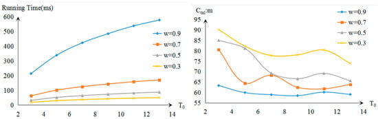
Figure 5. Running time and C_tnl values with different annealing speeds w and initial temperatures T₀.

The experimental results show that, when the initial temperature ${\mathrm{T}}_0$ is greater than 9, the correspondence effect has no obvious improvement. Given a rapid annealing speed, even when the initial temperature ${\mathrm{T}}_0$ is high enough, the correspondence effect is not acceptable. For example, when T₀ = 13 and w = 0.3, the C_tnl still has a large value of 73.94. When the annealing speed is slow enough, say w = 0.9, the corresponding results are satisfactory.

Considering the operation of map generalization, the matching algorithm performs well for the characteristic points generated by the vertex deletion, bend deletion and bend exaggeration operations. However, for the characteristic points generated by bend typification, the matching results are less satisfactory. For example, when ${\mathrm{T}}_0=9\mathrm{and}\mathrm{w}=0.9$, the segment between characteristic points ${\mathrm{b}}_{36}$ and ${\mathrm{b}}_{38}$ corresponds to a long segment at a large scale between vertexes ${\mathrm{v}}_{87}$ to ${\mathrm{v}}_{107}$, which results in merging two bends into a single bend. Nöellenburg et al. [13] believe that there is a trade-off between obtaining a smooth morph that retains the mental map and producing an optimal diagram at a fixed scale. If a user stops zooming at an intermediate scale where the merging process is not quite complete, it could make sense to continue merging while maintaining the scale until the representation of the bends is acceptable.

The process of piecewise linear interpolation is conducted based on the characteristic correspondence, of which the result is shown in Figure 6. Meanwhile, the same data were tested using the naive linear interpolation method; the results are shown in Figure 7. Based on this comparison, it can be seen that the SABM method produces gradual changes that involve vertex deletion, bend deletion and bend exaggeration. Even for bend typification, the SABM method merges two bends into a single bend, which is likely preferable. The morphing results produced by naive linear interpolation have two obvious defects. First, the isomorphic character of the two representations are broken during the interpolation; for example, the bend within the dotted rectangle first becomes exaggerated and then shrinks. On the other hand, using the SABM method, the bend was always constant. Second, the heterogeneous character of two representations generated by map generalization operations will not be able to reflect progressive changes. For example, the bend within the dotted circle becomes increasingly sharp, and it ceases to point to the right and begins to point upward. During the morphing process, the typification operation was not taken into consideration. The reason for the two abnormal deformations lies in that the naive linear interpolation method ignores the matching of the inherent structural characteristics of linear features. In contrast, the SABM method conducts a global optimal matching on each feature’s structural character, so the result is more acceptable and more adapted to human visual perception.

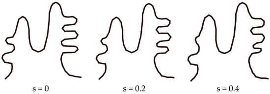
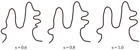
Figure 6. The morphing effect of the SABM method described in this paper.

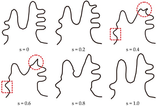
Figure 7. The morphing effect of naive linear interpolation.

3.2. The Application of SABM for Continuous Scale Transformation

Contours and river network are two typical linear features on maps. Here, the SABM method is applied to the continuous generalization of contours and river networks. The data set of contour lines has two scales, 1:10,000 and 1:50,000, and the data at these scales are generalized from the large-scale data. The scales of the river networks are 1:100,000 and 1:250,000. The complete data set comprises 17 contours and 57 rivers. Experiments similar to those described in Section 3.1 are performed to select the values of parameters T₀ and w. The experimental results show that the initial temperature parameter T₀ = 9 and annealing speed parameter w = 0.9 are suitable for morphing the contours and river network. The generalization effect are reflected by the average C_tnl values of the intermediate shape and the original shape in the coarser representation. Data sizes, running times and the series of C_tnl are given in Table 3. The morphing results are shown in Figure 8 and Figure 9, respectively. Actually the computation of the characteristic point extraction and optimum correspondence are part of the preprocessing of the data, whereas the actual morphing using straight-line trajectories is computed at interactive speeds. The statistical results in Table 3 show that when the value of s increases, the intermediate state is more and more like the original shape in the coarser representation as the value of C_tnl decreases. The SABM method can produce the continuous generalization of linear geographical features.

Table 3. Data sizes, running times and the series of C_tnl (in meters), (Num₁: number of records; Num₂: number of characteristic points; T₁: time to extract the critical points in seconds; T₂: time to determine the optimum correspondence in seconds).

	Num1	Num2	T1	T2	Ctnl (s = 0.2)	Ctnl (s = 0.4)	Ctnl (s = 0.6)	Ctnl (s = 0.8)
Contours	17	982	13.18	24.51	468	355	279	144
Rivers	57	212	2.71	5.7	399	307	226	136

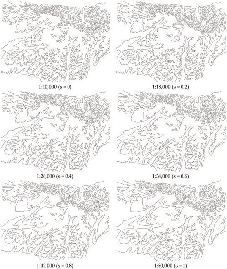
Figure 8. Contour morphing performed using the SABM method.

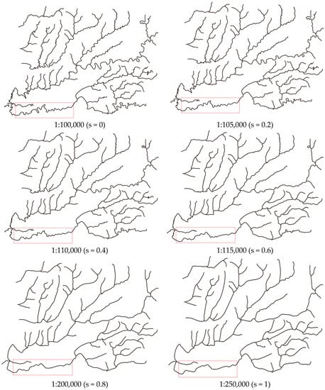
Figure 9. River network morphing generated by the SABM method.

4. Concluding Remarks

In this study, the morphing technique is used to perform the continuous generalization of linear features. In carrying out the morphing of vector data, there are two core processes, namely the matching of characteristic points and the interpolation of paths. In the context of map generalization, the two input states of finer and coarser polylines refer to the same entity, meaning that the two features have many common characteristics. By introducing the simulated annealing technique to perform the global correspondence of characteristic points, most of the homogeneous characteristics can be matched. The traditional map generalization operations, such as vertex deletion, bend deletion and the bend exaggeration effect can produce gradual warping effects in transformations from fine detail to coarse detail. If the coarser polyline being generated by bend typification operations, the correspondence relationship of the coarser and finer scales is an m-to-n mapping (where m and n denote the number of bend; m ≠ n), which means the finer state’s multiple bends may combine to the coarser state’s single bend. It is perhaps arguable whether this is the best correspondence, however. Experiments show that, when the initial temperature parameter T₀ = 9 and the annealing speed parameter w = 0.9, the corresponding results are satisfactory for most cases.

For the process of path interpolation, the linear interpolation method is employed. On the basis of the correspondence among characteristic points, the linear interpolation algorithm has been used to identify corresponding points for every pair of these split corresponding subpolylines, and the straight-line trajectories are employed for interpolation. The case study shows that the proposed method is accurate and efficient. Since the process of characteristic point extraction and corresponding takes structural information and the map generalization operations into account, this method can better preserve the gradual changes in homogeneous structures between two polylines in the interpolation process. Therefore, this method can improve the accuracy of morphing and can be used for the continuous generalization of linear geographic features.

However, the following two aspects still need to be improved. First, if the span over which the scale changes is large, the geometric dimensions of map objects may change, say from polygon to polyline. Thus, the SABM method cannot be used for this type of continuous generalization. Second, during the process of interpolation, non-linear trajectories can be developed to ensure that self-intersections do not occur.

References

- Bereuter, P.; Weibel, R. Real-time generalization of point data in mobile and web mapping using quadtrees. Cartogr. Geogr. Inf. Sci. 2013, 40, 271–281. [Google Scholar] [CrossRef]
- Meng, L.; Murphy, C.; Ding, L.; Yang, J. A Review of Research Works on VGI Understanding and Image Map Design. Kartographische Nachrichten. Available online: https://www.researchgate.net/publication/316277984_A_Review_of_Research_Works_on_VGI_Understanding_and_Image_Map_Design (accessed on 7 August 2017).
- Ai, T.H. The drainage network extraction from contour lines for contour line generalization. ISPRS J. Photogramm. Remote Sens. 2007, 62, 93–103. [Google Scholar] [CrossRef]
- Ai, T.H.; Li, J. A DEM generalization by minor valley branch detection and grid filling. ISPRS J. Photogramm. Remote Sens. 2010, 65, 198–207. [Google Scholar] [CrossRef]
- Jones, C.B.; Ware, J.M. Map generalization in the web age. Int. J. Geogr. Inf. Sci. 2005, 19, 859–870. [Google Scholar] [CrossRef]
- Danciger, J.; Devadoss, S.L.; Mugno, J.; Sheehy, D.; Ward, R. Shape deformation in continuous map generalization. Geoinformatica 2009, 13, 203–221. [Google Scholar] [CrossRef]
- Sester, M.; Brenner, C. Continuous generalization for visualization on small mobile devices. In Development of the Spatial Data Handling; Fisher, P., Ed.; Springer: Berlin/Heidelberg, Germany, 2005; pp. 355–368. [Google Scholar]
- Van Oosterom, P. Variable-scale Topological Data Structures Suitable for Progressive Data Transfer: The GAP-face Tree and GAP-edge Forest. Cartogr. Geogr. Inf. Sci. 2005, 32, 331–346. [Google Scholar] [CrossRef]
- Liu, P.C.; Li, X.G.; Liu, W.B.; Ai, T.H. Fourier based multi-scale representation and progressive transmission of cartographic curves on the internet. Cartogr. Geogr. Inf. Sci. 2016, 43, 454–468. [Google Scholar] [CrossRef]
- Ai, T.; Li, Z.; Liu, Y. Progressive Transmission of Vector Data Based on Changes Accumulation Model; SDH: Leicester, UK; Springer: Berlin, Germany, 2003; pp. 85–96. [Google Scholar]
- Van Kreveld, M. Smooth generalization for continuous zooming. In Proceedings of the 20th International Cartographic Conference (ICC’01), Beijing, China, 6–10 August 2001; pp. 2180–2185. [Google Scholar]
- Cecconi, A.; Galanda, M. Adaptive zooming in Web cartography. Comput. Graph. Forum 2002, 21, 787–799. [Google Scholar] [CrossRef]
- Nöellenburg, M.; Merrick, D.; Wolff, A.; Benkert, M. Morphing polylines: A step towards continuous generalization. Comput. Environ. Urban Syst. 2008, 32, 248–260. [Google Scholar] [CrossRef]
- Deng, M.; Peng, D. Morphing Linear Features Based on Their Entire Structures. Trans. GIS. 2015, 19, 653–677. [Google Scholar] [CrossRef]
- Whited, B.; Rossignac, J. B-morphs between b-compatible curves in the plane. In Proceedings of the ACM/SIAM Joint Conference on Geometric and Physical Modeling, San Francisco, CA, USA, 5–8 October 2009; pp. 187–198. [Google Scholar]
- Li, J.Z.; Li, X.G.; Xie, T. Morphing of Building Footprints Using a Turning Angle Function. ISPRS Int. J. Geo-Inf. 2017, 6, 173. [Google Scholar] [CrossRef]
- Yang, W.; Feng, J. 2D shape morphing via automatic feature matching and hierarchical interpolation. Comput. Graph. 2009, 33, 414–423. [Google Scholar] [CrossRef]
- Gomes, J.; Darsa, L.; Costa, B.; Velho, L. Warping and Morphing of Graphical Objects; Morgan Kaufman: San Francisco, CA, USA, 1999. [Google Scholar]
- Sederberg, T.; Greenwood, E. A physically based approach to 2D shape blending. ACM Comput. Graph. 1992, 26, 25–34. [Google Scholar] [CrossRef]
- Efrat, A.; Har-Peled, S.; Guibas, L.J.; Murali, T.M. Morphing between polylines. In Proceedings of the 12th ACM-SIAM Symposium on Discrete Algorithms, Washington, DC, USA, 7–9 January 2001; pp. 680–689. [Google Scholar]
- Van, O.R.; Veltkamp, R.C. Parametric search made practical. Comput. Geom. 2004, 28, 75–88. [Google Scholar]
- Sederberg, T.; Gao, P.; Wang, G.; Mu, H. 2-D shape blending: An intrinsic solution to the vertex path problem. Comput. Graph. 1993, 27, 15–18. [Google Scholar]
- Alexa, M.; Cohen-Or, D.; Levin, D. As-rigid-as-possible shape interpolation. In Proceedings of the 27th Annual Conference on Computer Graphics and Interactive Techniques (SIGGRAPH ’00), New Orleans, LA, USA, 23–28 July 2000; pp. 157–164. [Google Scholar]
- Surazhsky, V.; Gotsman, C. Intrinsic morphing of compatible triangulations. Int. J. Shape Model. 2003, 9, 191–201. [Google Scholar] [CrossRef]
- Ware, J.M.; Jones, C.B.; Thomas, N. Automated map generalization with multiple operators: A simulated annealing approach. Int. J. Geogr. Inf. Sci. 2003, 17, 743–769. [Google Scholar] [CrossRef]
- Kirkpatrick, S.; Gelattjr, C.D.; Vecchi, M.P. Optimization by Simulated Annealing. Science 1983, 220, 671–680. [Google Scholar] [CrossRef] [PubMed]
© 2017 by the authors. Licensee MDPI, Basel, Switzerland. This article is an open access article distributed under the terms and conditions of the Creative Commons Attribution (CC BY) license (http://creativecommons.org/licenses/by/4.0/).