Abstract
The relationship between burglary and socio-demographic factors has long been a hot topic in crime research. Spatial dependence and spatial heterogeneity are two issues to be addressed in modeling geographic data. When these two issues arise at the same time, it is difficult to model them simultaneously. A cross-comparison of three models is presented in this study to identify which spatial effect should be addressed first in crime analysis. The negative binominal model (NB), Bayesian hierarchical model (BHM) and the geographically weighted Poisson regression model (GWPR) were implemented based on a three-year residential burglary data set from ZG, China. The modeling result shows that both BHM and GWPR outperform NB as they capture either of the spatial effects. Compared to the NB model, the mean absolute deviation (MAD) of BHM and GWPR was decreased by 83.71% and 49.39%, the mean squared error (MSE) of BHM and GWPR was decreased by 97.88% and 77.15%, and the of BHM and GWPR was improved by 26.7% and 19.1%, respectively. In comparison with BHM and GWPR, BHM fits the data better with lower MAD, MSE and higher . The empirical analysis indicates that the percentage of renter population, percentage of people from other provinces, bus line density, and bus stop density have a significantly positive impact on the number of residential burglaries. The percentage of residents with a bachelor degree or higher, on the other hand, is negatively associated with the number of residential burglaries.
1. Introduction
Burglary has been a city problem for a long time. The spatial distribution of burglaries is never random. Some places are more prone to burglary than others. Much attention has been paid to the relationship between location and crime. Crime Prevention through Environmental Design (CPTED) has been considered as a necessary component in city planning in the western nations since 1970s.
Previous studies have widely examined the relationship between environmental characteristics and residential burglary. According to the social disorganization and routine activity theories, various environmental factors are found to be related to burglary, including road configurations [1,2], residential instability [3,4], demographics [5], income [6,7], unemployment rate [8], land use mix [9], housing characteristics [10,11,12,13], guardianship [14,15], accessibility [16], and the physical environment [17].
There are usually two kinds of data used for crime analysis in the literature, aggregate data and disaggregate data. Point data are referred to as disaggregate data because each point represents the location of an incident. Various approaches have been developed to analyze crime based on point data, such as kernel density [18,19,20] and Spatial Scan Statistics [20,21,22] for hot spot analysis. In order to investigate the relationship between crime events and the influential factors, crime incidents are usually aggregated into different spatial units, such as census tract or block groups. Two spatial effects, including spatial dependence and spatial heterogeneity, often arise after aggregation [23,24]. Spatial dependence shows how a geographic attribute exhibits similarity among the nearby locations [25]. Spatial heterogeneity or first-order non-stationarity, on the other hand, refers to the uneven distribution of spatial events or spatial relationships. In order to identify important underlying factors related to crime, multiple regression models have been widely used [26,27,28]. However, the independence assumption of the error distribution is often violated for spatial data due to spatial dependence. In addition, when the number of crimes is used as the dependent variable, the assumption of the normal distribution is violated because the number of crimes is a count variable. This will produce biased estimates due to the underestimated standard errors of regression coefficients [29].
A number of models have been proposed to overcome these problems. Spatial econometric models are employed to address spatial dependence, including the spatial error model and spatial lag model [30,31,32]. These two models also require the dependent variable to follow a continuous normal distribution. To satisfy this requirement, researchers often use the crime rate as the dependent variable, which has caused other issues. For example, the crime rate would become unstable where the population is low. Transforming the dependent variable, such as log-transformation, is another commonly used method to meet the assumption [33]. Unfortunately, transformation makes it difficult to interpret the model results [34].
Therefore, count data models are popular for crime analysis, and they can be either non-spatial or spatial. For example, Poisson [1] and negative binominal models [3,35] are two non-spatial count data models widely used in previous crime modeling. Two spatial count data models are the geographically weighted Poisson regression and Bayesian hierarchical model, which are described as follows.
Geographically weighted regression (GWR) was proposed by Fotheringham et al. [36] to handle spatial heterogeneity by allowing the relationship between variables to vary across a region. It is a powerful tool and is widely used in geographic research [37,38,39,40]. Similar to linear regression, the GWR model also requires normal distribution of the dependent variable. Geographically weighted Poisson regression (GWPR) is an extension of GWR for count data with a Poisson distribution [41].
The Bayesian hierarchical model (BHM) is another model proposed to address spatial autocorrelation by Besag for count data [42]. The BHM model handles data with Poisson or negative binominal distribution and has been widely used to analyze traffic crashes [43,44], crimes [45,46], and disease cases [47,48].
GWPR and BHM address spatial heterogeneity and spatial autocorrelation, respectively, but not both simultaneously. When spatial autocorrelation and heterogeneity occur at the same time, they cannot be independently modeled in a single model. To our best knowledge, there is no modeling methodology that can address these two problems at the same time. With a residential burglary data set collected in ZG, China, this research aims to identify the most suitable model for residential burglary by comparing the model fitness of three different models; the first one with no control for the spatial effects, the second one considering spatial dependence, and the third one accounting for spatial heterogeneity. In addition, this study enriches the existing literature on residential burglary from an empirical result obtained in a major city in China, which has unique socioeconomic characteristics and urban structure.
2. Methodology
The three tested models include the negative binomial model (NB), BHM, and GWPR. The NB model, which is non-spatial, is treated as the baseline. The BHM and GWPR models were calibrated to account for spatial dependence and spatial heterogeneity, respectively.
2.1. Negative Binominal Model
The Poisson distribution is often used as the benchmark for modeling count data. However, the basic assumption of the Poisson distribution is that the variance is equal to the mean, which is often not satisfied. When the variance is greater than the mean, the problem of over-dispersion arises, which is common in crime data. The negative binominal model is used to account for this issue.
Let denote the number of burglaries in spatial unit (= 1, 2, …, n), is the population used as the exposure variable of area , is the independent variable for area . The NB model is specified as:
where is the expected number of burglaries in area , ,…, are parameters, is a gamma-distributed error term with mean 1 and variance ; the additional term allows the variance different from the mean, as . The Poisson distribution is a special case of the negative binominal distribution when .
2.2. Bayesian Hierarchical Model
Though the NB model can address the over-dispersion issue, it cannot account for the spatial autocorrelation of burglary incidents. Based on the NB model, BHM was proposed to address spatial dependence among the adjacent zones by Besag et al. [42]. An error term and a conditional autoregressive prior are incorporated into the link function. The model specification is presented as follows:
where is the spatial autocorrelation. The conditional autoregressive prior used by previous studies [43,49] is adopted in this study:
in which is spatial adjacent matrix. If I and j share a border, , otherwise . is assumed to be a gamma prior with (0.5, 0.0005) as used in the literature [49,50]. The Markov Chain Monte Carlo (MCMC) algorithm could be used to estimate this model instead of the maximum likelihood estimation.
2.3. Geographically Weighted Poisson Regression (GWPR)
GWPR, proposed by Nakaya [51], was employed in this study to control for the spatial heterogeneity. The GWPR model, a variant of GWR for Poisson distribution data, has been used in road safety analysis [52]. The framework of GWPR is as follows:
where is the geographical coordinates of the centroid of spatial unit . is the coefficient of the th explanatory variable for zone which is a function of the centroid of spatial unit . This allows the parameter to vary across the area, and then the spatial heterogeneity is addressed. can be calculated by:
where is the vector of coefficients for spatial unit , is an n by n matrix for spatial weight, which is presented as:
where is the weight given to area I during the calibration procedure for area .
In GWPR, the regression coefficient associated with one spatial unit is estimated by the observations in the nearby units. This process is repeated for all spatial units. The weight of each unit is determined by the distance between it and the regression unit. Therefore, the observation closer to the regression unit has more influence on the coefficient estimation than the observations farther away. The magnitude of the influence is determined by the spatial weight matrix , which can be calculated by Gaussian or Bi-square kernel functions as follows:
Gaussian:
Bi-square:
where is the Euclidean distance between the centroids of unit and ; is known as the bandwidth. The result is largely determined by the bandwidth. As such, it is important to select a suitable bandwidth. The AIC (Akaike Information Criterion) is employed as the criterion for bandwidth selection. The lower the AIC value, the better the model fit.
2.4. Goodness of Fit
In order to compare the above-mentioned models’ performance, three evaluation criteria were employed to assess the goodness-of-fit of each model: , mean absolute deviation (MAD), and mean square error (MSE). The following is a detailed description of these criteria.
2.4.1. Mean Absolute Deviance (MAD)
The MAD measure is provided to evaluate model performance, which is the sum of the absolute differences between the predicted and the observed burglaries divided by the sample size. A smaller value of MAD means better model performance on average.
2.4.2. MSE
MSE is another measure to assess model performance, which is the average of the squared differences between the predicted and observed burglaries divided by the sample size.
Similar to the MAD measure, a smaller value of MSE suggests better model fitness.
2.4.3.
Non-linear models such as the negative binomial do not provide an overall model fitness measure such as R2. Based on the standardized residuals, Cameron and Windmeijer [53] proposed an indicator:
where and are the predicted burglaries obtained by the aforementioned models and the average burglary frequency, respectively. is the observed number of burglaries per spatial unit. Here, is the number of spatial units.
3. Study Area and Data
The crime in China has been increasing since the economic reform in the 1970s [54]. Burglary is the largest category of crime in China, accounting for 67.83% of total crime events [55]. Most previous burglary studies have focused on developed countries since the crime data are difficult to obtain in developing countries such as China. The crime data are confidential in many Chinese cities; therefore, the true name of the city is removed, and we call it ZG here.
3.1. Study Area
ZG is located in the southeast of China, the largest central city in Southern China. ZG covers an area of about seven thousand square kilometers and has attracted a large number of people for work due to the rapid economic development. More than sixteen million people lived in this city in 2015, about half are migrants from other cities or provinces.
Spatial units of different scales have been used in crime research, for example, countries, cities, census tracts, neighborhoods, and street segments. A typical city of China is divided into a number of small units named Police Station Management Areas (PSMAs). Each PSMA has a corresponding police station for the region’s crime prevention and control. There are 215 PSMAs in ZG, and crime incident data were aggregated into PSMAs in this analysis.
3.2. Data
The residential burglary data were obtained from the 110 reporting system of the municipal public security bureau; 110 is the emergency call for crime in China, similar to 911 in the U.S. Each record comes with many attributes, such as the unique number, the date, the name of the police station, and the crime category. These records were aggregated into PSMAs according to which police station it belongs. A three-year data set from 2013 to 2015 was used in this study. A total of 150113 burglaries were extracted from the reporting system (Figure 1). The number of burglaries in each PSMA varies from 0 to 3547.
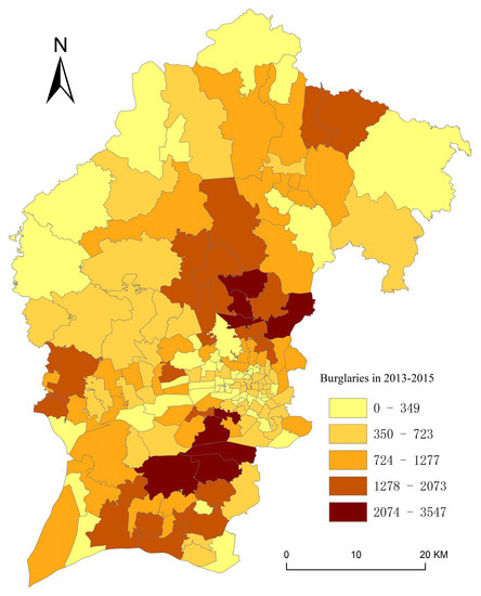
Figure 1.
Spatial distribution of residential burglaries in 2013–2015.
The explanatory variables used in this study were selected according to the routine activity theory [56] and social disorganization theory [57]. The routine activity theory claims that the concurrence of three determinants: attractive targets, absence of guardianship, and motivated offenders, will lead to a crime. The social disorganization theory argues that crimes are more likely to occur in socially disorganized neighborhoods. Nine variables were selected based on these two theories, which are described in detail as follows.
Income has been selected as the attractiveness for offenders in the literature since the motived criminals want to obtain as much as possible through a burglary [35,58]. Since there are no such data in the sixth census report of China, the percentage of large households which have an area greater than 120 m2 was used as a proxy for the household income instead. The level of education measures the variation in the education structure of the crime-prone population, but its impact was found to be mixed in the literature [14,58].
Guardianship can be divided into two categories including social guardianship and physical guardianship. The length of time that people stay at home can be seen as the social guardianship for an area. As such, the population below six or above sixty was used to represent social guardianship since these two groups spend more time at home than other age groups.
Residential instability has been employed as a measure to assess social disorganization in previous studies [3,16]. The percentage of renters and the percentage of migrants were included as two indices for the residential instability in this research.
Accessibility is important in the process of choosing a place to commit a crime [16]. The bus line density and bus stop density were used as indices for accessibility. The density of bus stop/bus lines was calculated as the total number of bus stops/bus lines divided by the road length in a PSMA. Table 1 provides the descriptive statistics of these variables. Multicollinearity between variables might lead to biased parameter estimates. A collinearity test was carried out before further analysis, and the results are shown in Table 2. The correlation coefficients between all variables are less than 0.7; therefore, there is no strong correlation between these variables.

Table 1.
Summary of Variable and Descriptive Statistics.
Table 2.
Results of the Correlation Matrix.
4. Results and Discussion
Three models were estimated for burglaries based on the previously mentioned methodology. This section compares model performance among the three models and discusses the factors that significantly influence burglaries in ZG.
4.1. Model Comparison
MAD, MSE and were calculated to compare the performance of the three models. Results in Table 3 shows that BHM is the strongest model with the lowest MAD, MSE and highest , followed by GWPR and NB, respectively. It is not surprising that the two spatial models, which take into account spatial correlation and heterogeneity, respectively, perform better than the non-spatial model.
Table 3.
Comparison between Models.
The Moran’s I statistics for all three model residuals are shown in Table 4. The model residuals of the negative binomial are significantly autocorrelated (p < 0.01), implying spatial correlation exists in the residuals and this will produce biased parameter estimates. With respect to the residuals of BHM and GWPR, no significant spatial autocorrelation is found. The results suggest that it is important to explicitly model the spatial effects to enhance model fitness, and that is why the two spatial models outperform the non-spatial model.
Table 4.
Moran’s I Test of Model Residuals.
The clustering pattern of residuals from the non-spatial model can be explained from the spatial distributions of dependent and independent variables. As summarized in Table 5, all variables show significant clustering patterns in space (p < 0.01), which might be caused by the clustered urban form. This again reinforces that the spatial effects should not be ignored in the models. The two significant HH local clusters and one LH outlier in the LISA map (Figure 2) imply that spatial dependence and heterogeneity exist and should be taken into account.
Table 5.
Moran’s I Statistics for Explanatory Variables.
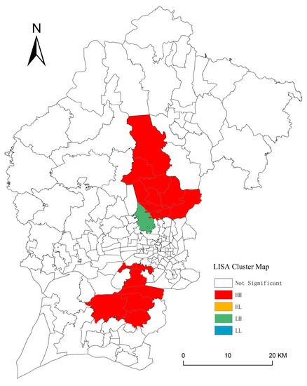
Figure 2.
Spatial clusters of residential burglaries during 2013–2015.
4.2. Parameter Estimation Comparison
The results of parameter estimation are shown in Table 6. The mean of the estimated coefficients is provided for NB and BHM. The minimum, lower quartile, median, upper quartile, and maximum of coefficients in GWPR are presented.
Table 6.
Model Results.
A comparison of BHM with GWPR and NB reveals that the coefficients of these three models are similar in magnitude and sign except for the sign of the resident with junior middle school education. This variable has a negative coefficient with no significance in the non-spatial model, but it turns out to be positive in the two spatial models. One possible explanation may be that the parameter estimate in the NB model is not accurate due to its failure to account for the spatial effects.
The percentage of large households is not significant in BHM. The impact of income on residential burglary is not consistent in the literature. Tseloni and Wittebrood [59] reported that income has a positive impact on burglary in the United Kingdom while the impact was negative in the United States. The study conducted by Malczewsk and Poetz [60] showed that areas with high burglary rates could be either poor or rich neighborhoods. In this research, the income is not a significant factor.
The bus line density and bus stop density are two indices for accessibility of an area. The relationship between accessibility and burglary also varies in the literature. Some studies found that areas with less accessibility may be at a higher risk to be victimized [61,62]. Others showed that accessibility was positively correlated with burglary [63], which is supported by the result from the BHM model. The positive relationship may be explained by the rational choice theory [56], which argues that offenders usually select households with higher accessibility as a target because of shorter entry and exit time. Higher accessibility of an area facilitates criminals to come and go easily, and this would motivate potential offenders.
Although past studies indicated that residential instability was not significantly associated with burglary [16,64], residential instability measured by the proportion of renters turned out to be significant in BHM. According to the social disorganization theory, homeowners are more concerned about the community security than renters; they are willing to improve the community instead of moving to another place like the renters. Thus, it is not a surprise that areas with more renters are at a higher risk of burglary. A few studies conducted in western nations also confirmed this finding [65,66].
Areas with a greater proportion of migrants are more prone to burglary. These people without local urban registration cannot share the equal opportunity for education and health services. According to the study conducted by Appleton and Song [67], most of the migrants are dissatisfied with their current status. ZG has a “floating population” of about 8 million, most of whom have limited education attainment and low income. Since these people cannot provide adequate security for their homes, they are more likely to be victims.
The percentage of residents with a bachelor’s degree or higher shows a significantly negative association with burglary, meaning a neighborhood dominated by residents with high education experiences less burglary. A similar conclusion was reached in other studies [14,68]. Very often, highly educated people can afford to improve their home security systems, such as surveillance cameras and alarms, which in turn would reduce the possibility of being victimized because of the enhanced high physical guardianship.
5. Conclusions
Because spatial autocorrelation and spatial heterogeneity are two important issues for crime modeling, many efforts have been made to address these two issues independently. However, it is not clear that controlling for a particular spatial effect will yield a stronger model. In this study, we quantitatively examined these two spatial effects in residential burglary modeling. Two different spatial techniques, GWPR and BHM, were used to address spatial heterogeneity and spatial autocorrelation, respectively, and they were compared to a non-spatial NB model. The BHM model was identified as the best model with the lowest MAD, MSE and highest . This empirical study suggests that modeling spatial dependence yields a better modeling result than modeling spatial heterogeneity.
It should be clarified that the intention of this research is not to prove that the BHM model always outperforms the GWPR model. Instead, we want to show that the spatial effects will be introduced when the individual data are aggregated, and it is important to model the spatial effects explicitly. The impact of these two spatial effects on the model fitness may vary with the datasets, and therefore, which spatial effect should be accounted for is the first issue to be addressed.
This research also identified important factors related to residential burglaries in a large city of China. The results reveal that the percentage of renters, percentage of people from other provinces, bus stop density, and bus routine density have a significantly positive impact on the number of burglaries. The percentage of people with a bachelor’s degree or higher has a significant yet negative correlation with burglary. Analyzing crime at a fine scale, such as at the PSMA scale, has great practical value because it can provide local operational decision support for law enforcement.
There are some limitations in this study. First, the mechanisms of these three models are different. Both NB and BHM are confirmative models, while GWPR is an explanatory model. Therefore, the three criteria used for comparison may not be complete. Assessment statistics for cross-comparison will be an important topic for future studies. Second, this analysis was based on the cumulative data over a three-year period, but the temporal dimension was not considered in the model. Further research will consider the spatial-temporal lag effect of burglary to expand our understanding of the linkage between residential burglary and sociodemographic and physical characteristics of a neighborhood.
Acknowledgments
This study was supported by a grant from a Key Program of the National Natural Science Foundation of China (Grant No. 41531178), the Natural Science Foundation of Guangdong Province (Grant No. 2014A030312010) and the National Natural Science Foundation for Outstanding Youth (Grant No. 41522104).
Author Contributions
Jianguo Chen and Lin Liu conceived and designed the study and wrote the manuscript. Jianguo Chen, Luzi Xiao and Guangwen Song carried out the experiment and analyzed the results. Suhong Zhou and Fang Ren provided key suggestions and helped with the writing of the manuscript. All authors have read and approved the final manuscript.
Conflicts of Interest
The authors declare no conflict of interest.
References
- Wu, L.; Liu, X.; Ye, X.; Leipnik, M.; Lee, J.; Zhu, X. Permeability, space syntax, and the patterning of residential burglaries in urban China. Appl. Geogr. 2015, 60, 261–265. [Google Scholar] [CrossRef]
- Davies, T.; Johnson, S.D. Examining the relationship between road structure and burglary risk via quantitative network analysis. J. Quant. Criminol. 2015, 31, 481–507. [Google Scholar] [CrossRef]
- Nobles, M.R.; Ward, J.T.; Tillyer, R. The impact of neighborhood context on spatiotemporal patterns of burglary. J. Res. Crime Delinquency 2016, 53, 711–740. [Google Scholar] [CrossRef]
- Montoya, L.; Junger, M.; Ongena, Y. The relation between residential property and its surroundings and day- and night-time residential burglary. Environ. Behav. 2016, 48, 515–549. [Google Scholar] [CrossRef]
- Liu, H.; Zhu, X. Exploring the influence of neighborhood characteristics on burglary risks: A Bayesian random effects modeling approach. ISPRS Int. J. Geo-Inf. 2016, 5, 102. [Google Scholar] [CrossRef]
- Parka, S.; Tarkb, J.; Choc, Y. Victimization immunity and lifestyle: A comparative study of over-dispersed burglary victimizations in South Korea and U.S. Int. J. Law Crime Justice 2016, 45, 44–58. [Google Scholar] [CrossRef]
- Tilley, N.; Tseloni, A.; Farrell, G. Income disparities of burglary risk: Security availability during the crime drop. Br. J. Criminol. 2011, 51, 296–313. [Google Scholar] [CrossRef]
- D’Alessio, S.J.; Eitle, D.; Stolzenberg, L. Unemployment, guardianship, and weekday residential burglary. Justice Q. 2012, 29, 919–932. [Google Scholar] [CrossRef]
- Sohn, D.W. Do all commercial land uses deteriorate neighborhood safety?: Examining the relationship between commercial land-use mix and residential burglary. Habitat Int. 2016, 55, 148–158. [Google Scholar] [CrossRef]
- Sidebottom, A. Repeat burglary victimization in Malawi and the influence of housing type and area-level affluence. Secur. J. 2012, 25, 265–281. [Google Scholar] [CrossRef]
- Zhang, H.; McCord, E.S. A spatial analysis of the impact of housing foreclosures on residential burglary. Appl. Geogr. 2014, 54, 27–34. [Google Scholar] [CrossRef]
- Vandevivera, C.; Neutensb, T.; van Daelea, S.; Geurtsc, D.; Bekena, T.V. A discrete spatial choice model of burglary target selection at the house-level. Appl. Geogr. 2015, 64, 24–34. [Google Scholar] [CrossRef]
- Coupe, T.; Blake, L. The effects of target characteristics on the sighting and arrest of offenders at burglary emergencies. Secur. J. 2011, 24, 157–178. [Google Scholar] [CrossRef]
- Addington, L.A.; Rennison, C.M. Keeping the barbarians outside the gate? Comparing burglary victimization in gated and non-gated communities. Justice Q. 2015, 32, 168–192. [Google Scholar] [CrossRef]
- Breetzke, G.D.; Cohn, E.G. Burglary in gated communities: An empirical analysis using routine activities theory. Int. Crim. Justice Rev. 2013, 23, 56–74. [Google Scholar] [CrossRef]
- Ward, J.T.; Nobles, M.R.; Youstin, T.J.; Cook, C.L. Placing the neighborhood accessibility–burglary link in social-structural context. Crime Delinquency 2014, 56, 739–763. [Google Scholar] [CrossRef]
- Breetzke, G.D. The effect of altitude and slope on the spatial patterning of burglary. Appl. Geogr. 2012, 34, 66–75. [Google Scholar] [CrossRef]
- Ye, X.; Xu, X.; Lee, J.; Zhu, X.; Wu, L. Space-time interaction of residential burglaries in Wuhan, China. Appl. Geogr. 2015, 60, 210–216. [Google Scholar] [CrossRef]
- Hodgkinson, T.; Andresen, M.A.; Farrell, G. The decline and locational shift of automotive theft: A local level analysis. J. Crim. Justice 2016, 44, 49–57. [Google Scholar] [CrossRef]
- Gorr, W.L.; Lee, Y.J. Early warning system for temporary crime hot spots. J. Quant. Criminol. 2015, 31, 25–47. [Google Scholar] [CrossRef]
- Quick, M.; Law, J. Exploring hotspots of drug offences in Toronto: A comparison of four local spatial cluster detection methods. Can. J. Criminol. Crim. Justice 2013, 55, 215–238. [Google Scholar] [CrossRef]
- Shiode, S. Street-level spatial scan statistic and STAC for analysing street crime concentrations. Trans. GIS 2011, 15, 365–383. [Google Scholar] [CrossRef]
- Lesage, J.P. The Theory and Practice of Spatial Econometrics; University of Toledo: Toledo, OH, USA, 1999. [Google Scholar]
- António, M.R.; José, A.T. Sensitivity analysis of spatial autocorrelation using distinct geometrical settings: Guidelines for the quantitative geographer. Int. J. Agric. Environ. Inf. Syst. (IJAEIS) 2016, 7, 65–77. [Google Scholar]
- Tobler, W.R. A computer movie simulating urban growth in the detroit region. Econ. Geogr. 1970, 46, 234–240. [Google Scholar] [CrossRef]
- Meško, G.; Fallshore, M.; Muratbegović, E.; Fields, C. Fear of crime in two post-socialist capital cities—Ljubljana, Slovenia and Sarajevo, Bosnia and Herzegovina. J. Crim. Justice 2008, 36, 546–553. [Google Scholar]
- Cahill, M.E.; Mulligan, G.F. The determinants of crime in tucson, arizona. Urban Geogr. 2003, 24, 582–610. [Google Scholar] [CrossRef]
- Dewan, A.M.; Haider, M.R.; Amin, M.R. Exploring crime statistics. In Dhaka Megacity: Geospatial Perspectives on Urbanisation, Environment and Health; Springer: Dordrecht, The Netherlands, 2014; pp. 257–282. [Google Scholar]
- Law, J.; Haining, R. A Bayesian approach to modeling binary data: The case of high-intensity crime areas. Geogr. Anal. 2004, 36, 197–216. [Google Scholar] [CrossRef]
- Hirschfield, A.; Birkin, M.; Brunsdon, C.; Malleson, N.; Newton, A. How places influence crime: The impact of surrounding areas on neighborhood burglary rates in a british city. Urban Stud. 2014, 51, 1057–1072. [Google Scholar] [CrossRef]
- Andresen, M.A. The ambient population and crime analysis. Prof. Geogr. 2011, 63, 193–212. [Google Scholar]
- Breetzke, G. Modeling violent crime rates: A test of social disorganization in the city of Tshwane, South Africa. J. Crim. Justice 2010, 38, 446–452. [Google Scholar] [CrossRef]
- Qian, X.; Ukkusuri, S.V. Spatial variation of the urban taxi ridership using GPS data. Appl. Geogr. 2015, 59, 31–42. [Google Scholar] [CrossRef]
- Robert, B.; O’Hara, D.; Kotze, J. Do not log-transform count data. Methods Ecol. Evol. 2010, 1, 118–122. [Google Scholar]
- Hunter, J.; Tseloni, A. Equity, justice and the crime drop: The case of burglary in England and Wales. Crime Sci. 2016, 5, 1–13. [Google Scholar] [CrossRef]
- Fotheringham, A.S.; Brunsdon, C.; Charlton, M. Geographically Weighted Regression: The Analysis of Spatially Varying Relationships; John Wiley & Sons Ltd.: Chichester, UK, 2002. [Google Scholar]
- Bagheri, N.; Holt, A.; Benwell, G.L. Using geographically weighted regression to validate approaches for modelling accessibility to primary health care. Appl. Spat. Anal. Policy 2009, 2, 177–194. [Google Scholar] [CrossRef]
- Chen, D.; Truong, K. Using multilevel modeling and geographically weighted regression to identify spatial variations in the relationship between place-level disadvantages and obesity in Taiwan. Appl. Geogr. 2012, 32, 737–745. [Google Scholar] [CrossRef]
- Corner, R.J.; Dewan, A.M.; Hashizume, M. Modelling typhoid risk in Dhaka Metropolitan Area of Bangladesh: The role of socio-economic and environmental factors. Int. J. Health Geogr. 2013, 12, 13. [Google Scholar] [CrossRef] [PubMed]
- Dewan, A.M.; Corner, R.; Hashizume, M.; Ongee, E.T. Typhoid fever and its association with environmental factors in the dhaka metropolitan area of bangladesh: A spatial and Time-Series approach. PLoS Negl. Trop. Dis. 2013, 7, e1998. [Google Scholar] [CrossRef] [PubMed]
- Li, Z.; Wang, W.; Liu, P.; Bigham, J.M.; Ragland, D.R. Using geographically weighted poisson regression for county-level crash modeling in California. Saf. Sci. 2013, 58, 89–97. [Google Scholar] [CrossRef]
- Besag, J. Spatial interaction and the statistical analysis of lattice systems. J. R. Stat. Soc. 1974, 36, 192–236. [Google Scholar]
- Amoh-Gyimah, R.; Saberi, M.; Sarvi, M. Macroscopic modeling of pedestrian and bicycle crashes: A cross-comparison of estimation methods. Accid. Anal. Prev. 2016, 93, 147–159. [Google Scholar] [CrossRef] [PubMed]
- Wang, X.; Yang, J.; Lee, C.; Ji, Z.; You, S. Macro-level safety analysis of pedestrian crashes in Shanghai, China. Accid. Anal. Prev. 2016, 96, 12–21. [Google Scholar] [CrossRef] [PubMed]
- Law, J.; Chan, P.W. Bayesian spatial random effect modelling for analysing burglary risks controlling for offender, socioeconomic, and unknown risk factors. Appl. Spat. Anal. Policy 2012, 5, 73–96. [Google Scholar] [CrossRef]
- Gracia, E.; López-Quílez, A.; Marco, M.; Lladosa, S.; Lila, M. Exploring neighborhood influences on small-area variations in intimate partner violence risk: A bayesian random-effects modeling approach. Int. J. Environ. Res. Public Health. 2014, 11, 866–882. [Google Scholar] [CrossRef] [PubMed]
- Hu, Y.; Ward, M.P.; Xia, C.; Li, R.; Sun, L.; Lynn, H.; Gao, F.; Wang, Q.; Zhang, S.; Xiong, C.; et al. Monitoring schistosomiasis risk in East China over space and time using a Bayesian hierarchical modeling approach. Sci. Rep. 2016, 6, 1–9. [Google Scholar] [CrossRef] [PubMed]
- Wong, R.S.Y.; Ismail, N.A. An application of Bayesian approach in modeling risk of death in an intensive care unit. PLoS ONE 2016, 11, 1–17. [Google Scholar] [CrossRef] [PubMed]
- Quddus, M.A. Modelling area-wide count outcomes with spatial correlation and heterogeneity: An analysis of London crash data. Accid. Anal. Prev. 2008, 40, 1486–1497. [Google Scholar] [CrossRef] [PubMed]
- Lee, J.; Abdel-Aty, M.; Jiang, X. Multivariate crash modeling for motor vehicle and non-motorized modes at the macroscopic level. Accid. Anal. Prev. 2015, 78, 146–154. [Google Scholar] [CrossRef] [PubMed]
- Nakaya, T.; Fotheringham, A.S.; Brunsdon, C.; Charlton, M. Geographically weighted Poisson regression for disease association mapping. Stat. Med. 2005, 24, 2695–2717. [Google Scholar] [CrossRef] [PubMed]
- Shariat-Mohaymany, A.; Shahri, M.; Mirbagheri, B.; Matkan, A.A. Exploring spatial non-stationarity and varying relationships between crash data and related factors using geographically weighted poisson regression. Trans. GIS 2015, 19, 321–337. [Google Scholar] [CrossRef]
- Cameron, A.C.; Windmeijer, F.A.G. R-squared measures for count data regression models with applications to health-care utilization. J. Bus. Econ. Stat. 1996, 14, 209–220. [Google Scholar] [CrossRef]
- Zhang, L.; Messner, S.F.; Liu, J. A multilevel analysis of the risk of household burglary in the city of Tianjin, China. Br. J. Criminol. 2007, 47, 918–937. [Google Scholar] [CrossRef]
- Bureau, C.S. China Statistical Yearbook; Statistical Publishing House: Beijing, China, 2015. [Google Scholar]
- Cohen, L.E.; Felson, M. Social change and crime rate trends: A routine activity approach. Am. Sociol. Rev. 1979, 44, 588–608. [Google Scholar] [CrossRef]
- Shaw, R.C.; McKay, D.H. Juvenile Delinquency and Urban Areas; University of Chicago Press: Chicago, IL, USA, 1942. [Google Scholar]
- Badiora, A.I.; Oluwadare, D.B.; Dada, O.T. Nature of residential burglary and prevention by design approaches in a nigerian traditional urban center. J. Appl. Secur. Res. 2014, 9, 418–436. [Google Scholar] [CrossRef]
- Tseloni, A.; Wittebrood, K.; Farrell, G.; Pease, K. Burglary victimization in england and wales, the united states and the netherlands: A cross-national comparative test of routine activities and lifestyle theories. Br. J. Criminol. 2004, 44, 66–91. [Google Scholar] [CrossRef]
- Malczewski, J.; Poetz, A. Residential burglaries and neighborhood socioeconomic context in London, Ontario: Global and local regression analysis. Prof. Geogr. 2005, 57, 516–529. [Google Scholar] [CrossRef]
- Hillier, B. Can streets be made safe? Urban Des. Int. 2004, 9, 31–45. [Google Scholar] [CrossRef]
- Shu, S.C. Housing layout and crime vulnerability. Urban Des. Int. 2000, 5, 177–188. [Google Scholar]
- Chang, D. Social crime or spatial crime? Exploring the effects of social, economical, and spatial factors on burglary rates. Environ. Psychol. Nonverbal Behav. 2011, 43, 26–52. [Google Scholar] [CrossRef]
- Bernasco, W.; Nieuwbeerta, P. How do residential burglars select target areas?: A new approach to the analysis of criminal location choice. Br. J. Criminol. 2005, 45, 296–315. [Google Scholar] [CrossRef]
- Wickes, R.; Hipp, J.R.; Sargeant, E.; Homel, R. Collective efficacy as a task specific process: Examining the relationship between social ties, neighborhood cohesion and the capacity to respond to violence, delinquency and civic problems. Am. J. Community Psychol. 2013, 52, 115–127. [Google Scholar] [CrossRef] [PubMed]
- Lindblad, R.M.; Manturuk, R.K.; Quercia, G.R. Sense of community and informal social control among lower income households: The role of homeownership and collective efficacy in reducing subjective neighborhood crime and disorder. Am. J. Community Psychol. 2013, 51, 123–139. [Google Scholar] [CrossRef] [PubMed]
- Appleton, S.; Song, L. Life satisfaction in urban china: Components and determinants. World Dev. 2008, 36, 2325–2340. [Google Scholar] [CrossRef]
- Law, J.; Quick, M. Exploring links between juvenile offenders and social disorganization at a large map scale: A Bayesian spatial modeling approach. J. Geogr. Syst. 2013, 15, 89–113. [Google Scholar] [CrossRef]
© 2017 by the authors. Licensee MDPI, Basel, Switzerland. This article is an open access article distributed under the terms and conditions of the Creative Commons Attribution (CC BY) license (http://creativecommons.org/licenses/by/4.0/).