

4SIM: A Novel Description Model for the Ternary Spatial Relation “Between” of Buildings


Abstract
1. Introduction
2. Related Works
2.1. Spatial Relations
2.2. Higher-Order Spatial Relations
2.3. “Between” Spatial Relation Models
3. Description Method for the Ternary Spatial Relation “Between” of Buildings
3.1. The 4SIM Model
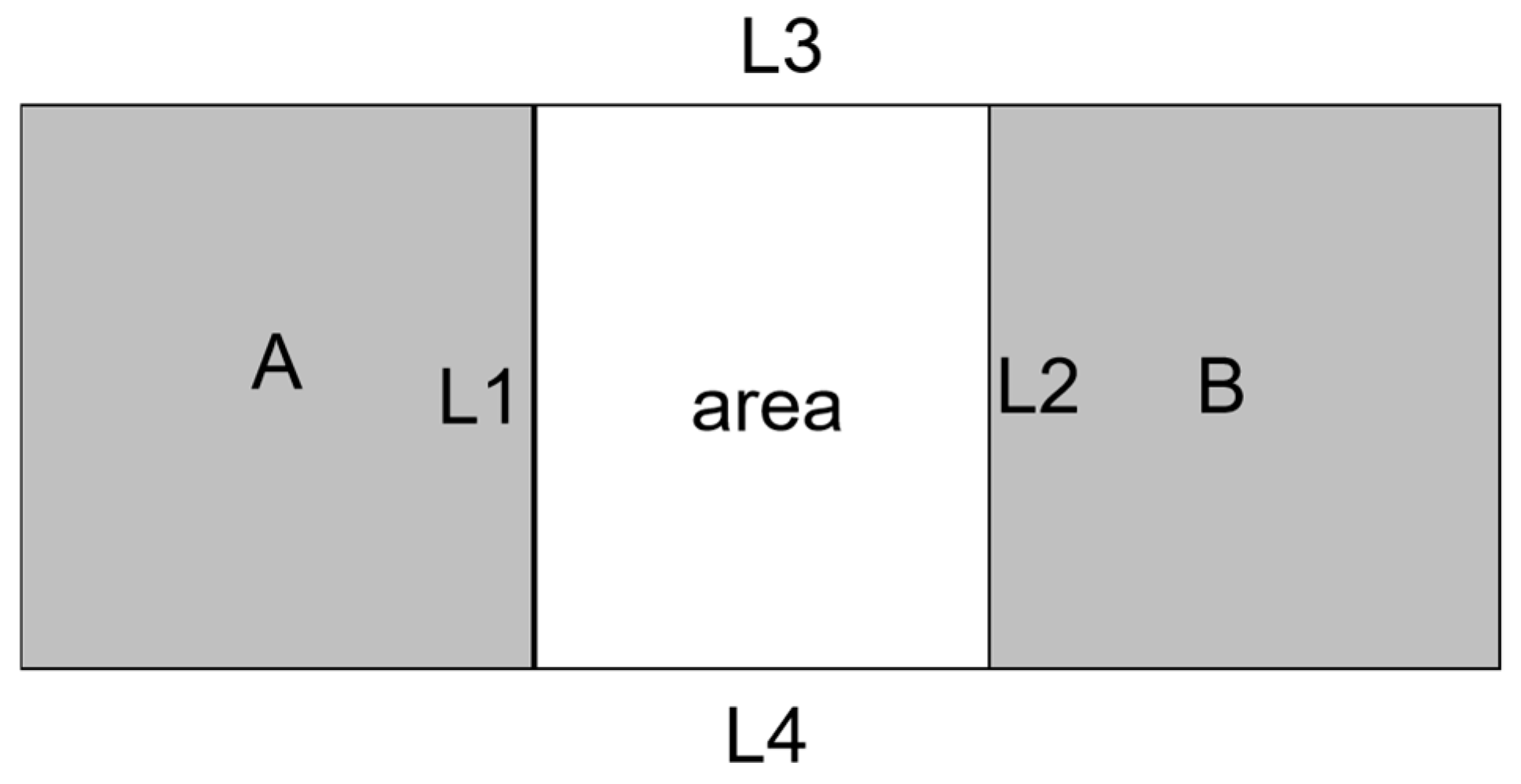
- is the intersection of object A with , where ;
- is the intersection of object B with , where ;
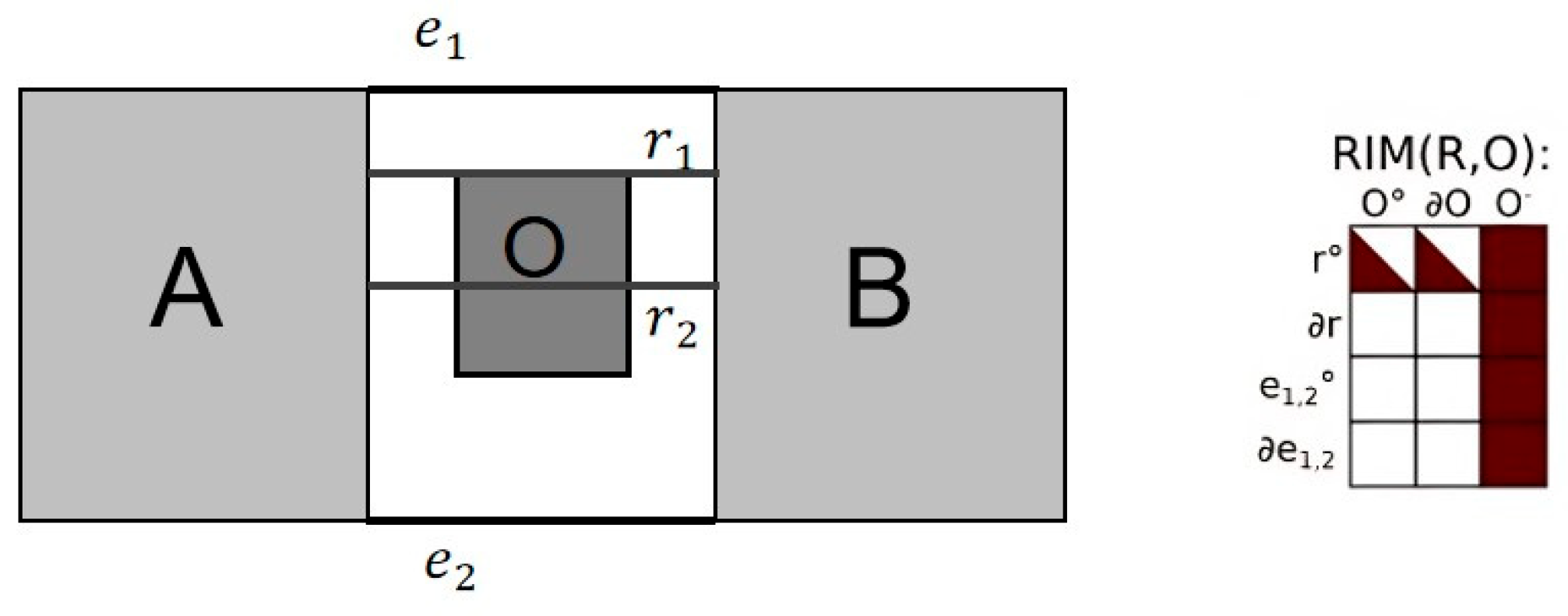
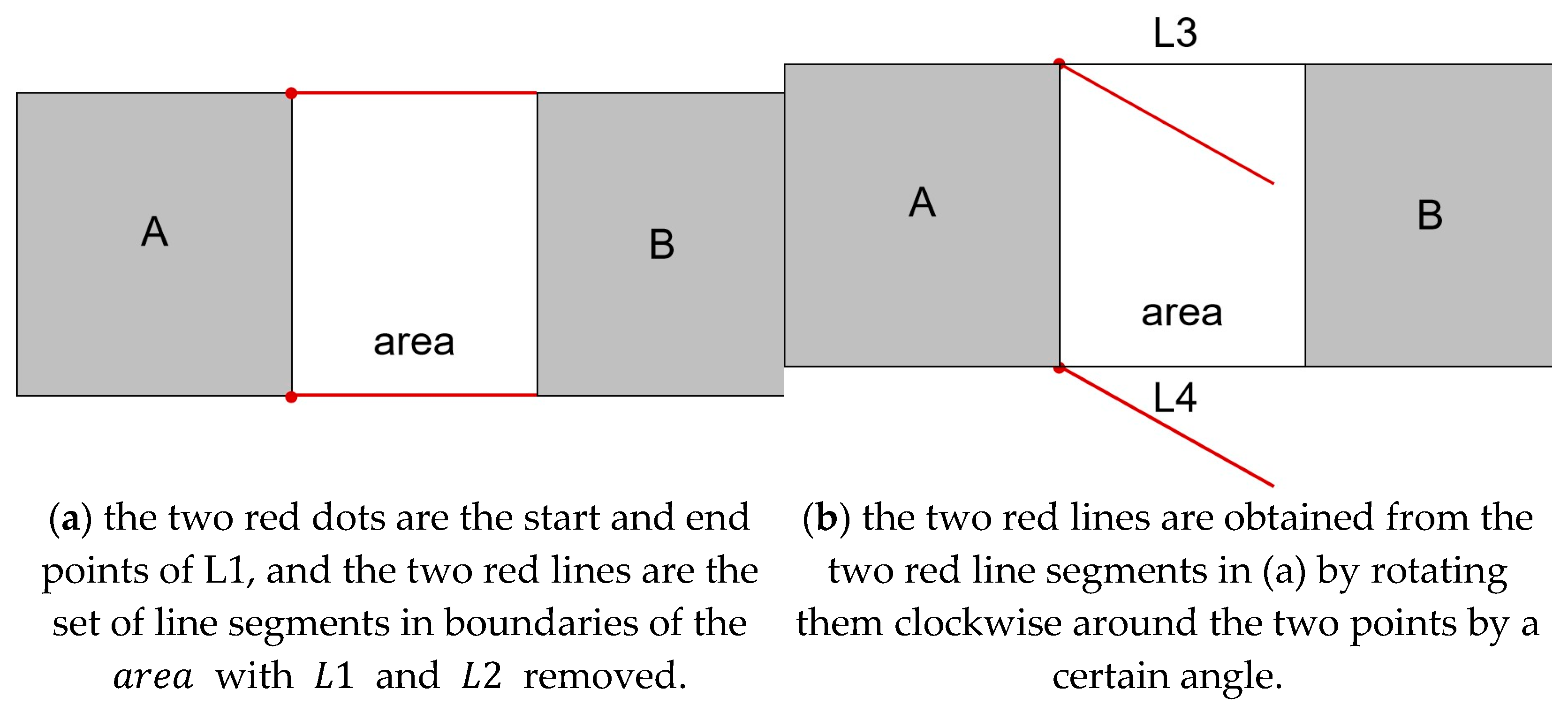
- and are the boundaries of the that intersect with A and B, respectively. is clockwise of and is clockwise of .
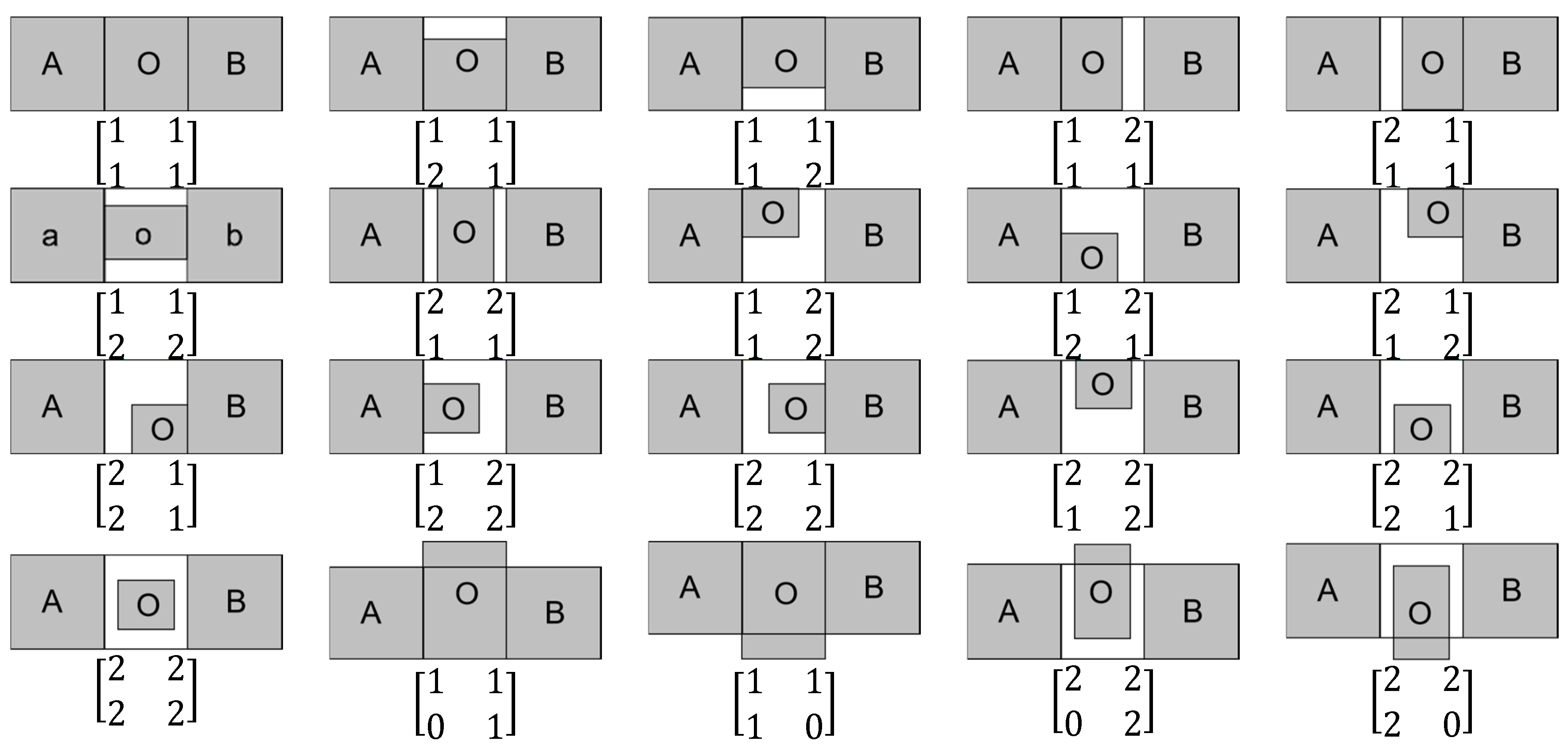
- i.
- When object O is inside the constrained region or is covered by the constrained region or is equal to it, that is, if the 9IM of the spatial relations between O and the constrained region are or or the topological relation between and O is denoted as 1 or 2, namely, . There are in total cases.
- ii.
- When object O intersects with the constrained region, that is, if the 9IM of the spatial relation between O and the constrained region is , and are topologically met or disjointed from O, denoted as or . or are topologically connected to O, denoted as , and another boundary line is topologically connected to O, denoted as , , or . That is, . There are in total cases.
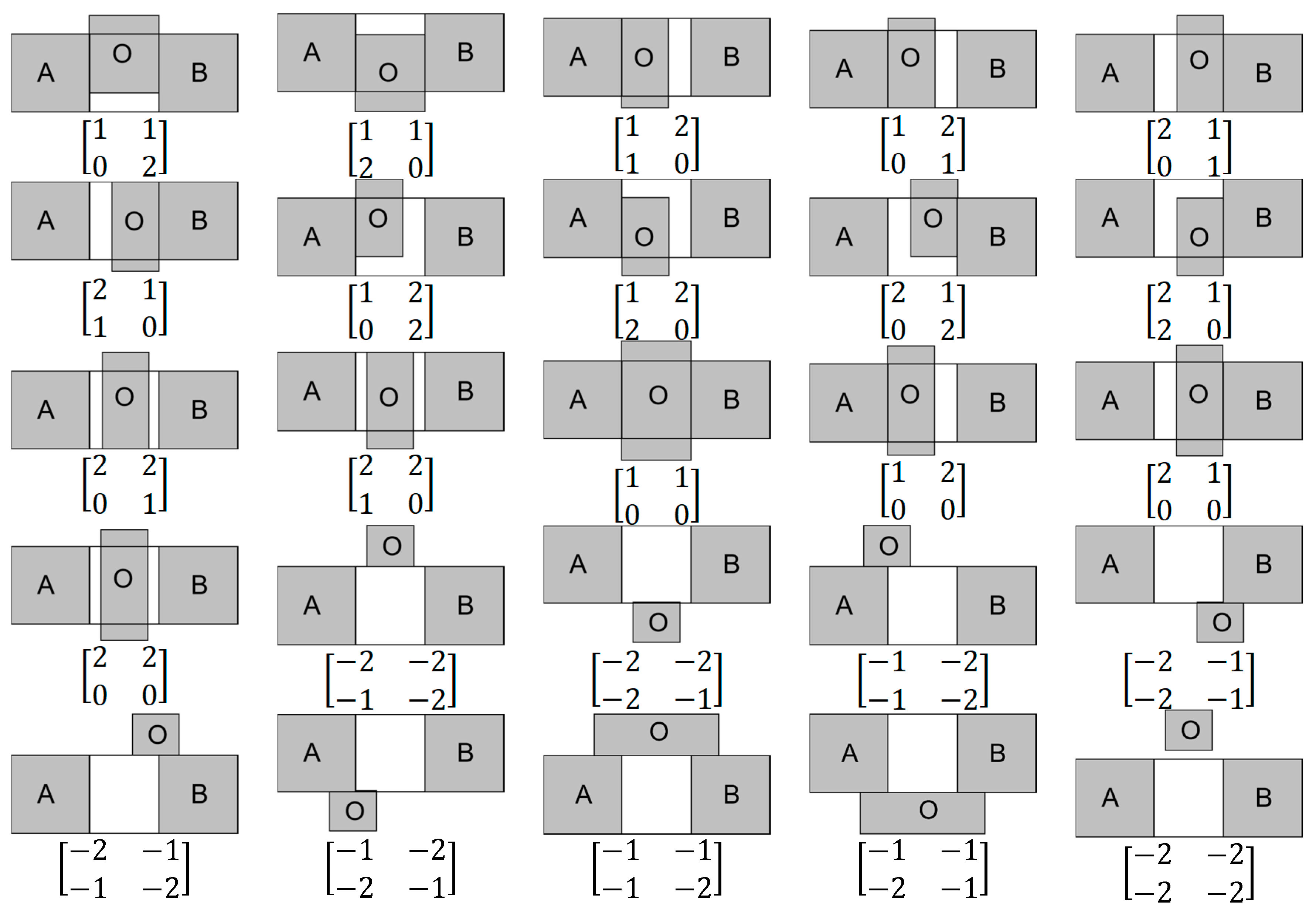
- iii.
- When object O is separated from or in contact with the constrained region, the 9IM of spatial relations between O and the constrained region are or , the topological relation between and , and O is denoted as or . When one of them is , the other must be . In this case, the topological relation between and and O is denoted as or . When both of them are , the topological relation between and and O is denoted as . That is, . There are in total cases.
3.2. 4SIM Performance Analysis
- i.
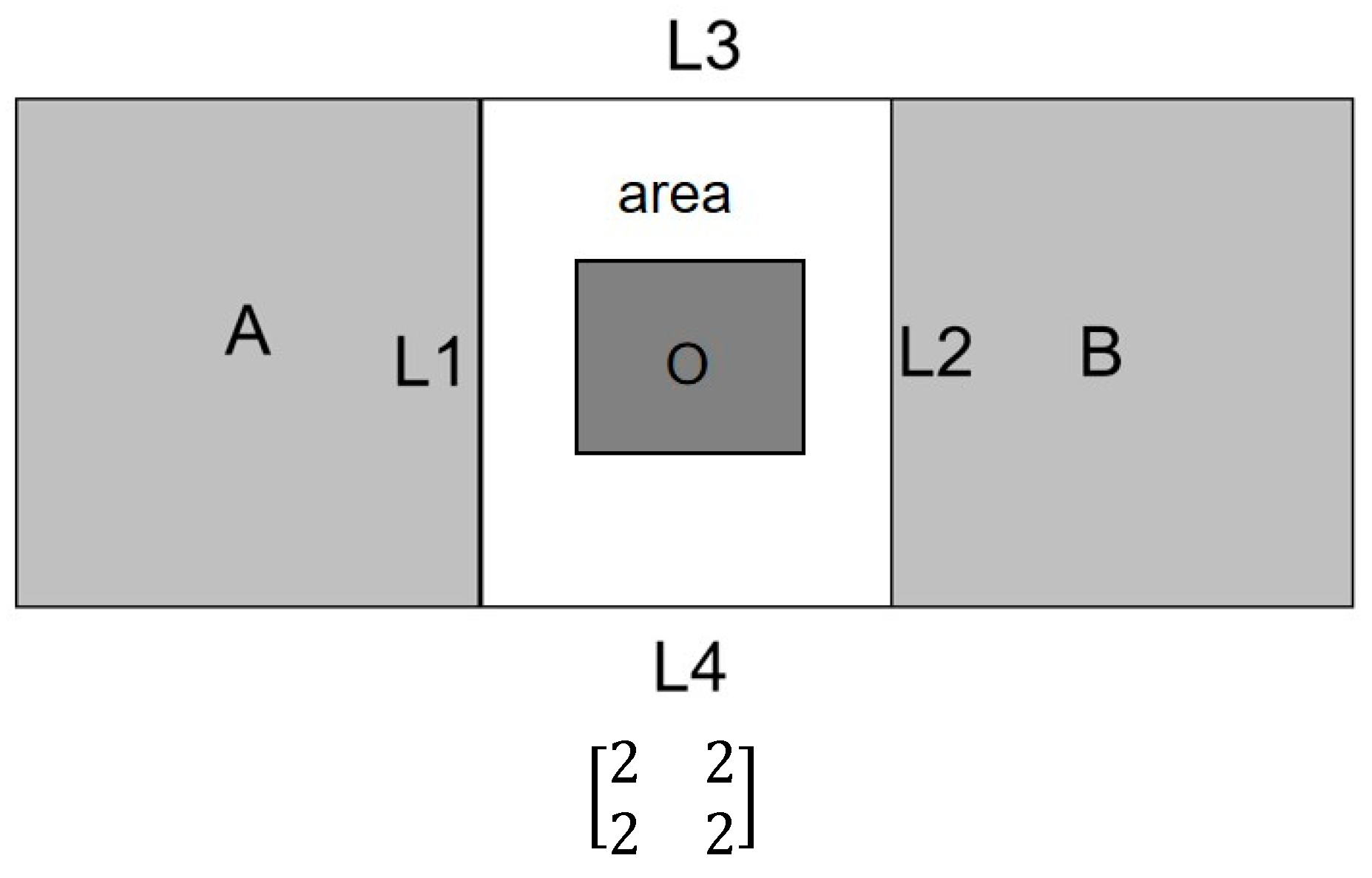
- The first is when O is completely between A and B, i.e., .
- ii.
- The second is when O is partially between A and B, i.e., .
- iii.
- The third is that O is not between A and B, i.e., .
4. 4SIM Implementation Methodology
4.1. Calculation of the Region Between A and B
4.2. Identification of the Four Boundaries
| Algorithm 1. Calculation of the region between A and B, and L1, L2, L3, L4 | |
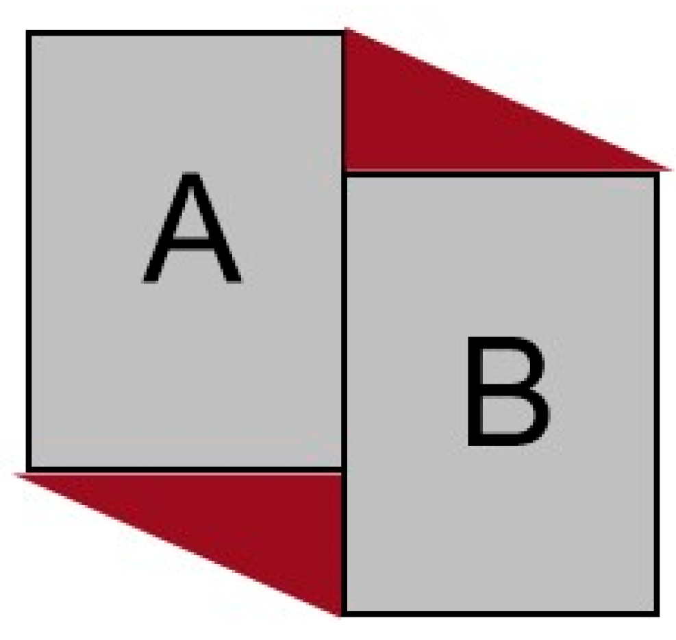
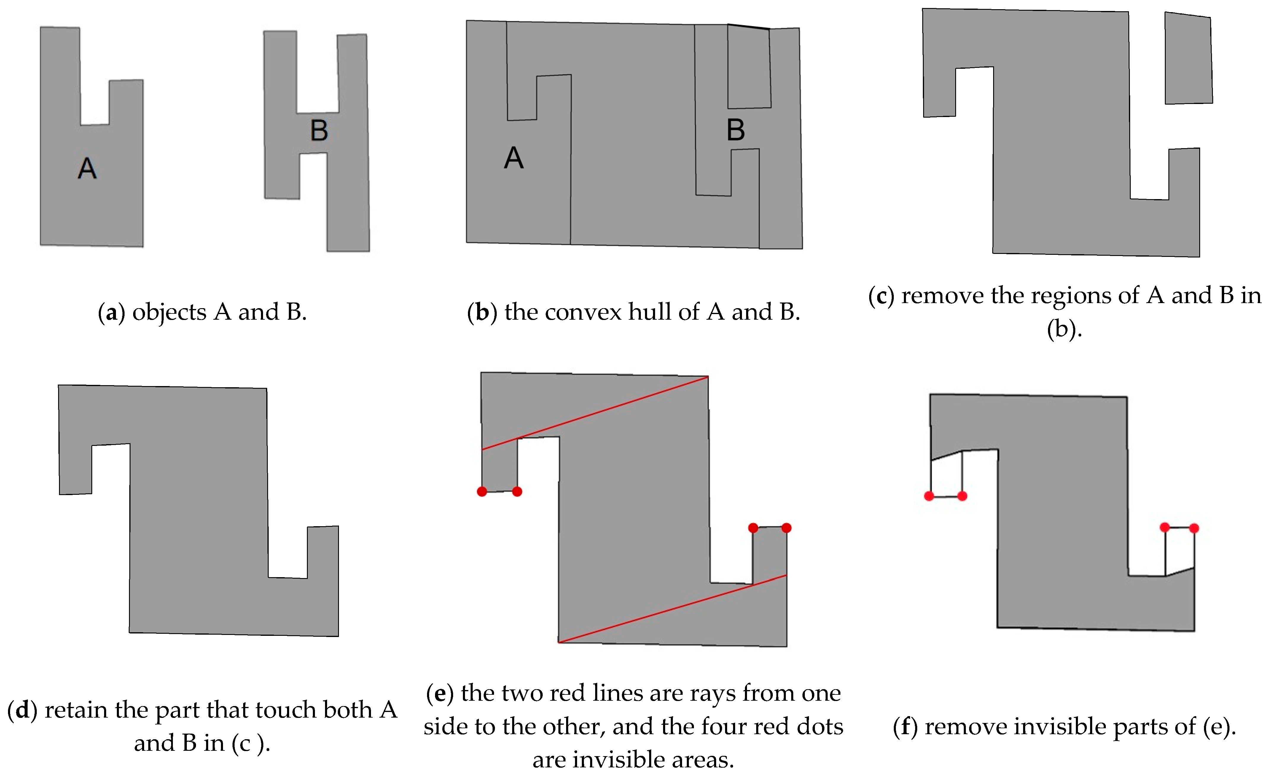
| # Step 1: Find the convex hull of A and B | 1 |
| convex_hull_ = convex_hull(A, B) () | 2 |
| 3 | |
| # Step 2: Remove A and B’s regions | 4 |
| area = convex_hull_.difference(A).difference(B) | 5 |
| 6 | |
| # Step 3: Delete the part that touches only A or B, and keep the part that touches both A and B | 7 |
| for geom in list(area): | 8 |
| if geom.disjoint(A) or geom.disjoint(B): | 9 |
| area.remove(geom) | 10 |
| 11 | |
| # Step 4: Find L1 and L2 | 12 |
| L1 = A.intersection(O) | 13 |
| L2 = B.intersection(O) | 14 |
| 15 | |
| # Step 5: Start and end of L1 line segment | 16 |
| start_point_L1, end_point_L1 = find_start_end_points(L1) | 17 |
| 18 | |
| # Step 6 Find the line segment set in area except L1 and L2 | 19 |
| remaining_lines = area.boundary.difference(L1).difference(L2) | 20 |
| 21 | |
| # Step 7: Rotate the segment set clockwise around the starting point | 22 |
| rotated_lines = rotate_lines(remaining_lines, start_point_L1, 1) | 23 |
| 24 | |
| #Step 8: Determine whether the rotated line segment intersects the area | 25 |
| L3 = [] | 26 |
| L4 = [] | 27 |
| for line in rotated_lines: | 28 |
| if is_intersect(line, area): | 29 |
| L3.append(line) | 30 |
| else: | 31 |
| L4.append(line) | 32 |
5. Comparative Experiment and Discussion
5.1. Combination of Ternary Buildings
5.2. Experiments
5.3. Discussion and Analysis
- (1)
- Comparison of distinguishing ability with existing models
- (2)
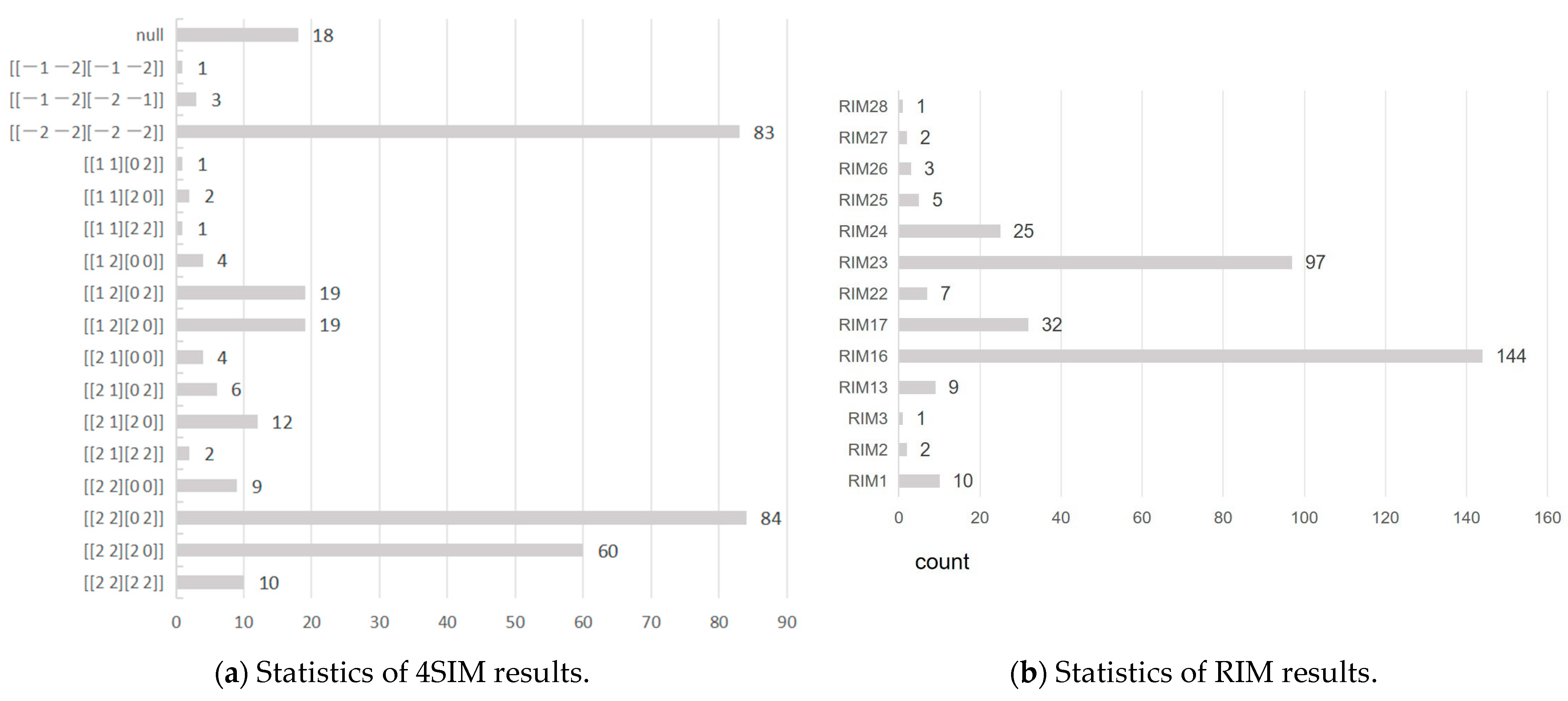
- Analysis of the “” results
- (3)
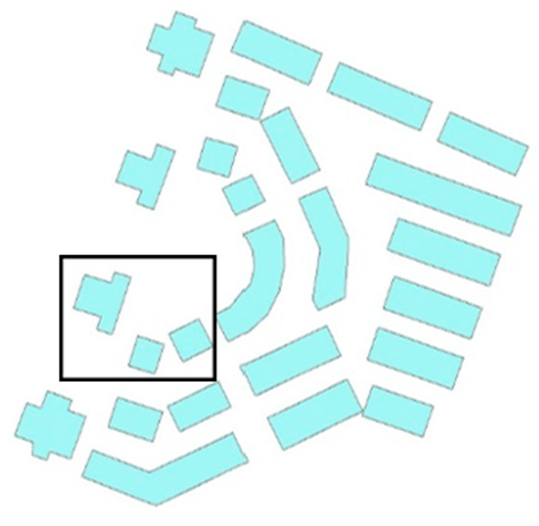
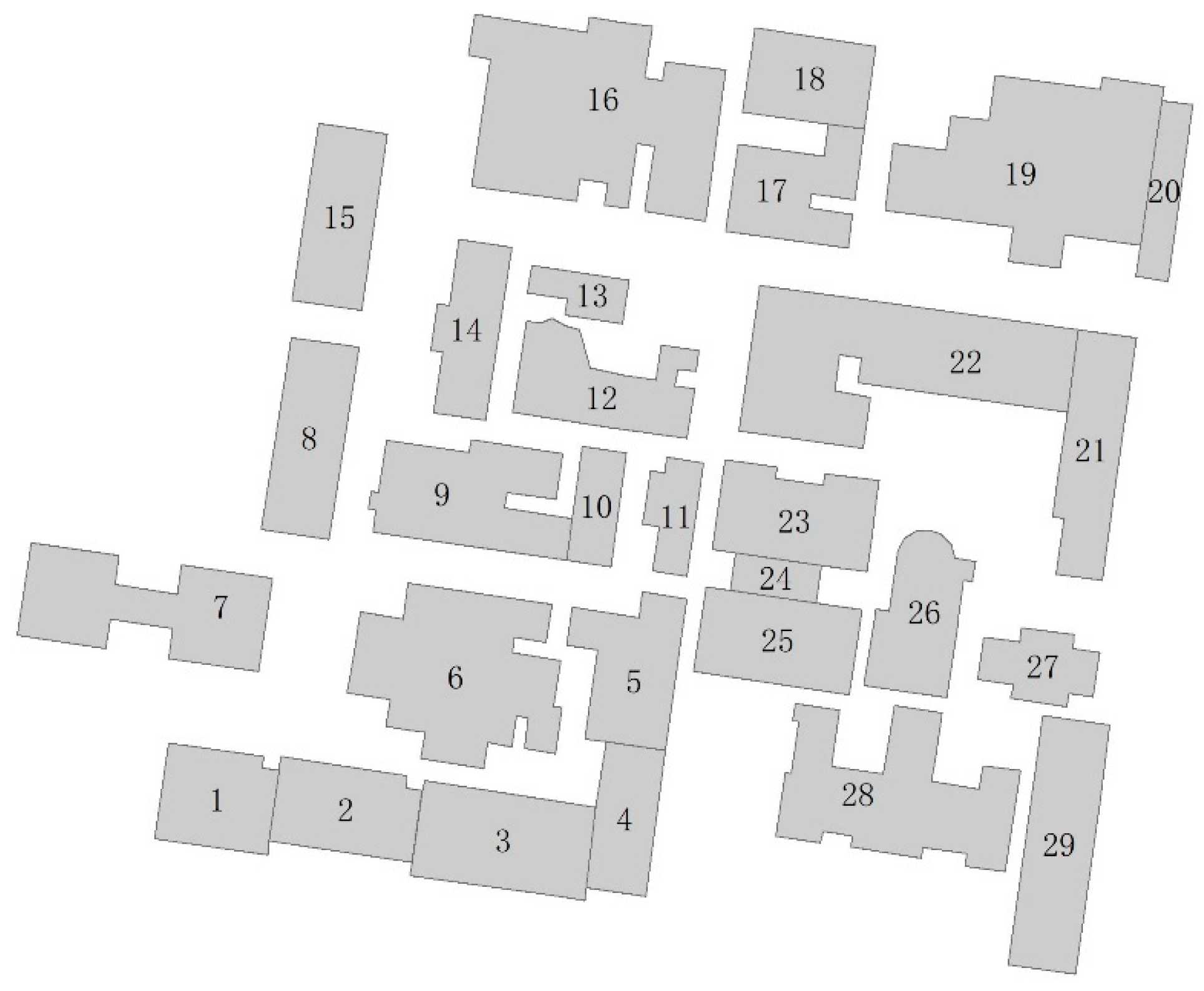
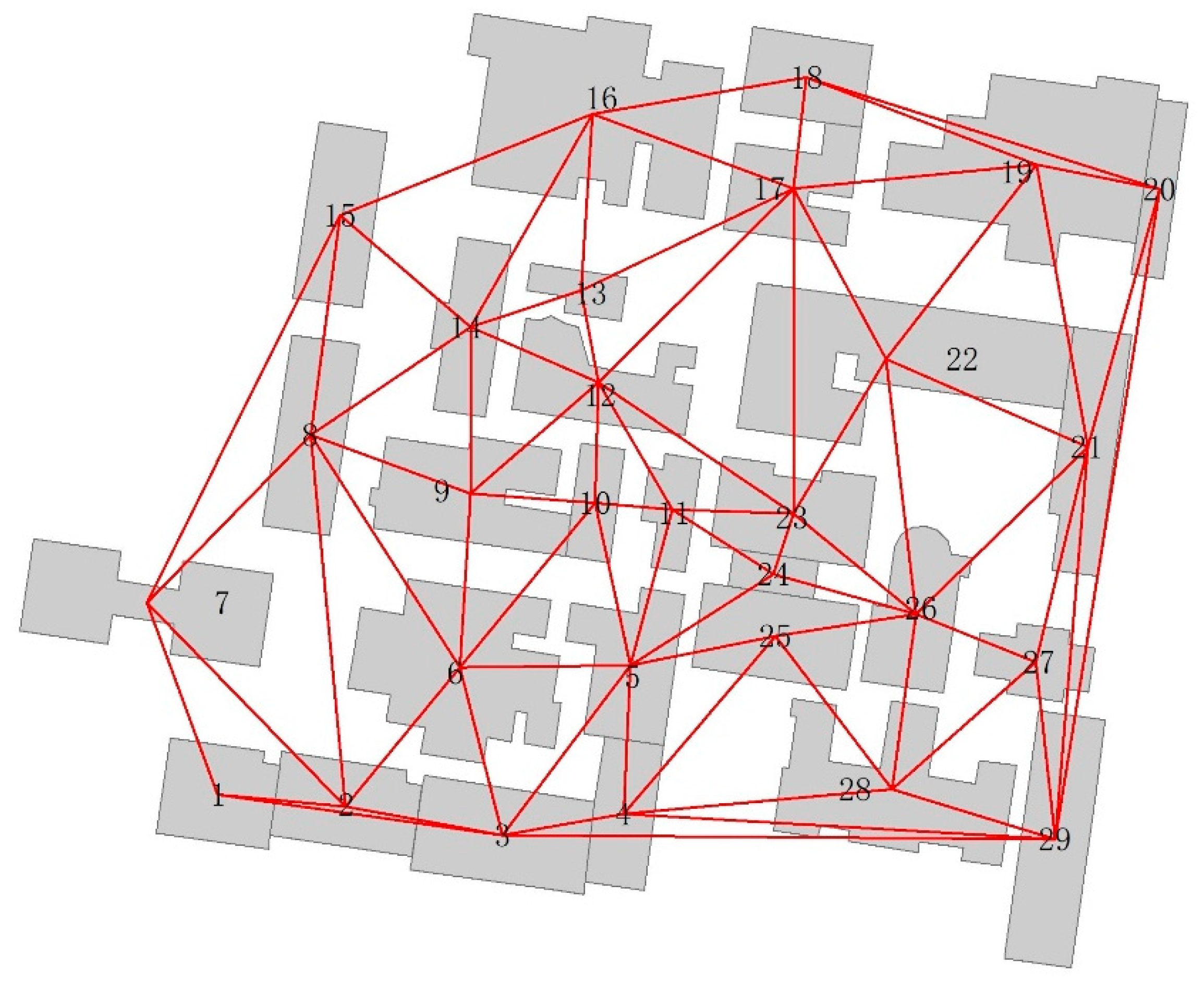
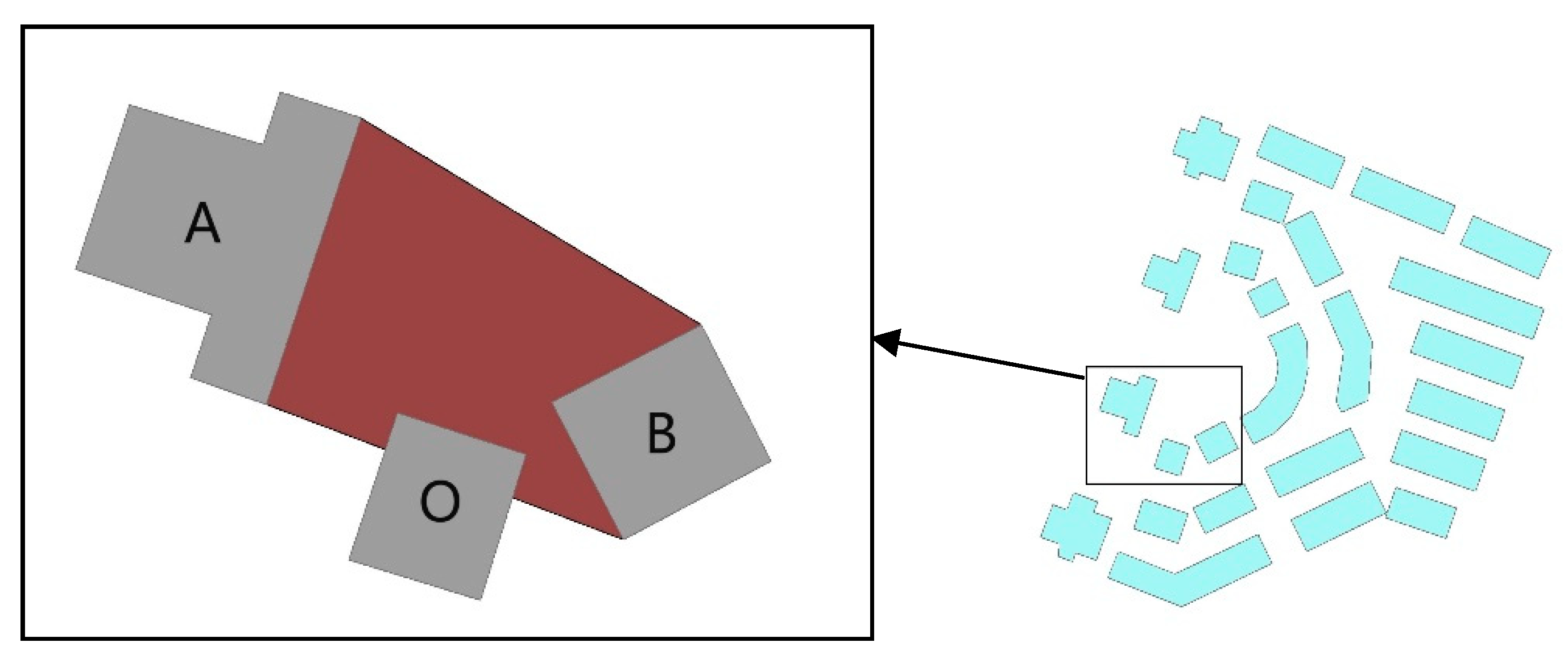
- Description for spatial distribution of irregular buildings
6. Conclusions
Author Contributions
Funding
Data Availability Statement
Conflicts of Interest
References
- Stell, J.G. Part and Complement: Fundamental Concepts in Spatial Relations John G. Stell Ann. Math. Artif. Intell. 2004, 41, 1–17. [Google Scholar] [CrossRef]
- Wu, K.; Zhang, X.; Dang, Y.; Ye, P. Deep Learning Models for Spatial Relation Extraction in Text. Geo-Spat. Inf. Sci. 2022, 26, 58–70. [Google Scholar] [CrossRef]
- van der Ham, I.J.M.; Borst, G. The Nature of Categorical and Coordinate Spatial Relation Processing: An Interference Study. J. Cogn. Psychol. 2011, 23, 922–930. [Google Scholar] [CrossRef]
- Xu, M.; Xie, Z. Hierarchical Spatial Proximity Reasoning for Vision-and-Language Navigation. IEEE Robot. Autom. Lett. 2024, 9, 10756–10763. [Google Scholar] [CrossRef]
- Zhang, X.; Ai, T.; Stoter, J.; Kraak, M.-J.; Molenaar, M. Building pattern recognition in topographic data: Examples on collinear and curvilinear alignments. Geoinformatica 2013, 17, 1–33. [Google Scholar] [CrossRef]
- He, X.; Zhang, X.; Xin, Q. Recognition of building group patterns in topographic maps based on graph partitioning and random forest. ISPRS J. Photogramm. Remote Sens. 2018, 136, 26–40. [Google Scholar] [CrossRef]
- Wang, X.; Burghardt, D. Using stroke and mesh to recognize building group patterns. Int. J. Cartogr. 2019, 6, 71–98. [Google Scholar] [CrossRef]
- Gong, X.; Wu, F. A Graph Match Approach to Typical Letter-like Pattern Recognition in Urban Building Groups. Geomat. Inf. Sci. Wuhan Univ. 2018, 43, 159–166. [Google Scholar]
- Du, S.; Luo, L.; Cao, K.; Shu, M. Extracting building patterns with multilevel graph partition and building grouping. ISPRS J. Photogramm. Remote Sens. 2016, 122, 81–96. [Google Scholar] [CrossRef]
- Zhao, R.; Ai, T.; Yu, W.; He, Y.; Shen, Y. Recognition of building group patterns using graph convolutional network. Cartogr. Geogr. Inf. Sci. 2020, 47, 400–417. [Google Scholar] [CrossRef]
- Worboys, M.; Duckham, M. Qualitative-geometric ‘surrounds’ relations between disjoint regions. Int. J. Geogr. Inf. Sci. 2021, 35, 1032–1063. [Google Scholar] [CrossRef]
- Bloch, I.; Colliot, O.; Cesar, R.M., Jr. On the Ternary Spatial Relation “Between”. IEEE Trans. Syst. Man Cybern. Part B (Cybern.) 2006, 36, 312–327. [Google Scholar] [CrossRef] [PubMed]
- Majic, I.; Naghizade, E.; Winter, S.; Tomko, M. RIM: A ray intersection model for the analysis of the between relationship of spatial objects in a 2D plane. Int. J. Geogr. Inf. Sci. 2020, 35, 893–918. [Google Scholar] [CrossRef]
- Takemura, C.M.; Cesar, R.M., Jr.; Bloch, I. Modeling and measuring the spatial relation ‘‘along’’: Regions, contours and fuzzy sets. Pattern Recognit. 2012, 45, 757–766. [Google Scholar] [CrossRef]
- Corcoran, P.; Mooney, P.; Bertolotto, M. Spatial Relations Using High Level Concepts. ISPRS Int. J. Geo-Inf. 2012, 1, 333–350. [Google Scholar] [CrossRef]
- Du, S.; Luo, L.; Zhao, W.; Guo, Z. Research Progress in Multi-scale Spatial Relations. J. Geo-Inf. Sci. 2015, 17, 135–146. [Google Scholar]
- Randell, D.A.; Cui, Z.; Cohn, A.G. A spatial logic based on regions and connection. Int. Conf. Princ. Knowl. Represent. Reason. 1992, 92, 165–176. [Google Scholar]
- Egenhofer, M.J.; Franzosa, R.D. Point Set Topological Spatial Relations. Int. J. Geogr. Inf. Syst. 1991, 5, 161–174. [Google Scholar] [CrossRef]
- Egenhofer, M.J.; Herring, J. Categorizing binary topological relations between regions, lines and points in geographic databases. Santa Barbar. CA Natl. Cent. Geogr. Inf. Anal. Tech. Rep. 1990, 94, 1–28. [Google Scholar]
- Clementini, E.; Felice, P.D. A model for representing topological relationships between complex geometric features in spatial databases. Inf. Sci. 1996, 90, 121–136. [Google Scholar] [CrossRef]
- Chen, J.; Li, C.; Li, Z. Improving 9-intersection model by replacing the complement with voronoi region. Geo-Spat. Inf. Sci. 2000, 3, 1–10. [Google Scholar]
- Du, S.; Wang, Q.; Li, Z. Definitions of Natural-Language Spatial Relations in GIS. Geomat. Inf. Sci. Wuhan Univ. 2005, 30, 533–538. [Google Scholar]
- Zhang, x.; Lv, G. Natural-language Spatial Relations and Their Applications in GIS. J. Geo-Inf. Sci. 2007, 9, 77–81. [Google Scholar]
- Freksa, C. Using Orientation Information for Qualitative Spatial Reasoning; Springer: Berlin/Heidelberg, Germany, 1992; pp. 162–178. [Google Scholar]
- Freksa, C. Temporal reasoning based on semi-intervals. Artif. Intell. 1992, 54, 199–227. [Google Scholar] [CrossRef]
- Clementini, E.; Billen, R. Modeling and Computing Ternary Projective Relations between Regions. IEEE Trans. Knowl. Data Eng. 2006, 18, 799–814. [Google Scholar] [CrossRef]
- Clementini, E. Projective Relations on the Sphere; Springer: Berlin/Heidelberg, Germany, 2008; pp. 313–322. [Google Scholar]
- Xu, N.; Majic, I.; Tomko, M. Perceptions of Qualitative Spatial Arrangements of Three Objects. In Leibniz International Proceedings in Informatics (LIPIcs); Schloss Dagstuhl—Leibniz-Zentrum für Informatik: Kobe, Japan, 2022; Volume 240, pp. 9:1–9:14. [Google Scholar]


| A | B | O | A | B | O | A | B | O |
|---|---|---|---|---|---|---|---|---|
| 1 | 2 | 3 | 1 | 3 | 2 | 2 | 3 | 1 |
| 2 | 1 | 3 | 3 | 1 | 2 | 3 | 2 | 1 |
| RIM | 4SIM | 338 | |
| Runtime: 27.933 ms | Runtime: 23.925 ms | ||
| RIM1 | 10 | O is completely between A and B | |
| RIM2 | 2 | ||
| RIM3 | 1 | ||
| RIM13 | 9 | O is partially between A and B | |
| RIM16 | 84 + 40 = 144 | ||
| RIM17 | 11 + 9 + 4 + 7 + 1 = 32 | ||
| RIM22 | 3 + 1 + 3 = 7 | O is not between A and B | |
| RIM23 | 83 + 14 = 97 | ||
| RIM24 | 8 + 10 + 2 + 5 = 25 | O is partially between A and B | |
| RIM25 | 3 + 2 = 5 | ||
| RIM26 | 1 + 2 = 3 | ||
| RIM27 | 2 | ||
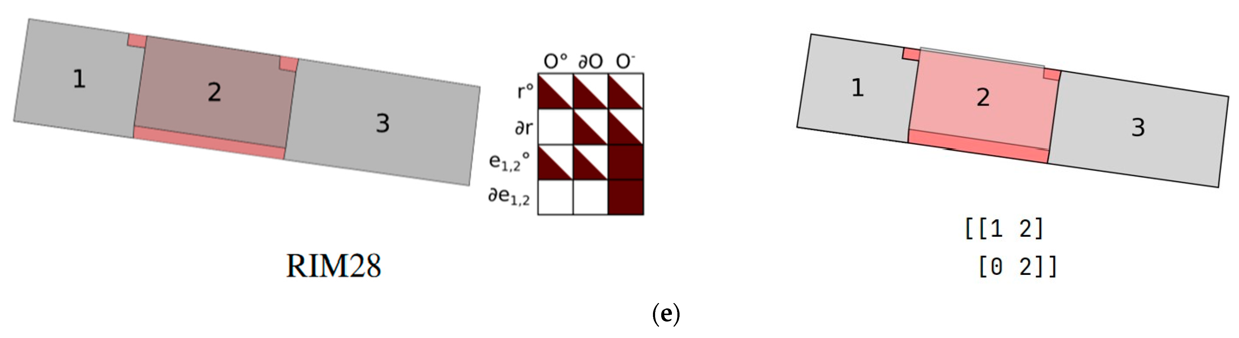
| RIM28 | 1 |
Disclaimer/Publisher’s Note: The statements, opinions and data contained in all publications are solely those of the individual author(s) and contributor(s) and not of MDPI and/or the editor(s). MDPI and/or the editor(s) disclaim responsibility for any injury to people or property resulting from any ideas, methods, instructions or products referred to in the content. |
© 2025 by the authors. Published by MDPI on behalf of the International Society for Photogrammetry and Remote Sensing. Licensee MDPI, Basel, Switzerland. This article is an open access article distributed under the terms and conditions of the Creative Commons Attribution (CC BY) license (https://creativecommons.org/licenses/by/4.0/).
Share and Cite
Zhang, H.; Gong, X.; Liu, C.; Wu, F.; Qiu, Y.; Wang, A.; Qi, Y. 4SIM: A Novel Description Model for the Ternary Spatial Relation “Between” of Buildings. ISPRS Int. J. Geo-Inf. 2025, 14, 83. https://doi.org/10.3390/ijgi14020083
Zhang H, Gong X, Liu C, Wu F, Qiu Y, Wang A, Qi Y. 4SIM: A Novel Description Model for the Ternary Spatial Relation “Between” of Buildings. ISPRS International Journal of Geo-Information. 2025; 14(2):83. https://doi.org/10.3390/ijgi14020083
Chicago/Turabian StyleZhang, Hanxue, Xianyong Gong, Chengyi Liu, Fang Wu, Yue Qiu, Andong Wang, and Yuyang Qi. 2025. "4SIM: A Novel Description Model for the Ternary Spatial Relation “Between” of Buildings" ISPRS International Journal of Geo-Information 14, no. 2: 83. https://doi.org/10.3390/ijgi14020083
APA StyleZhang, H., Gong, X., Liu, C., Wu, F., Qiu, Y., Wang, A., & Qi, Y. (2025). 4SIM: A Novel Description Model for the Ternary Spatial Relation “Between” of Buildings. ISPRS International Journal of Geo-Information, 14(2), 83. https://doi.org/10.3390/ijgi14020083