A Methodology to Convert Highly Detailed BIM Models into 3D Geospatial Building Models at Different LoDs

Abstract

This paper presents an implemented methodology to convert highly detailed building information models (BIMs) into geospatial 3D city models (Geos) at multiple levels of detail (LoDs). As BIM models contain highly detailed and complex geometries that differ significantly from city model standards, abstraction and conversion methods are required to generate usable outputs. Our study addresses this by developing a methodology that generates nine different LoDs from a single IFC input. These LoDs include both volumetric and surface-based abstractions for exterior and interior representations. The methodology involves voxelisation, filtering and simplification of surfaces, footprint derivation, storey abstraction, and interior geometry extraction. Together, these approaches allow flexible conversion tailored to specific applications, balancing accuracy, complexity, and computational efficiency. The methodology is implemented in a prototype tool named IfcEnvelopeExtractor. It automates IFC-to-CityGML/CityJSON conversion with minimal user input. The methodology was tested on a variety of models ranging from small houses to multistorey buildings. The evaluation covered geometric accuracy, semantic accuracy, and model complexity. Results show that non-volumetric abstractions and interior abstractions performed very well, producing robust and accurate results. However, the accuracy decreased for volumetric and complex abstractions, particularly at higher LoDs. Problems included missing or incorrectly trimmed surfaces, and modelling gaps and tolerance issues in the input IFC models. These limitations reveal that the quality of the input BIM models significantly affects the reliability of conversions. Overall, the methodology demonstrates that automated, flexible, and open-source solutions can effectively bridge the gap between BIM and geospatial domains, contributing to scalable GeoBIM integration in practice.

1. Introduction

Building information modelling (BIM) and geoinformation are widely recognised as complementary sources of data. Whereas a BIM model can represent a single building or infrastructure project in high detail, geoinformation-based sources can represent different types of features in a large region with less detail. Integrating geoinformation and BIMs is very useful in practice and constitutes an active research field which is often referred to as GeoBIM. A short list of GeoBIM applications include performing checks for the issuance of building permits using buildings (BIM) and city regulations (Geo), navigation that combines outdoor (Geo) and indoor (BIM) portions, facility management for infrastructure sites (BIM) that include the regional connections between the sites (Geo), and risk management using regional simulations (Geo) that also takes into account the impact on specific sites (BIM).

Among the geoinformation datasets that are usually considered within a GeoBIM context, 3D city models stand out because they model buildings in three dimensions, making them analogous to BIM models of buildings. Converting BIM to 3D city models has a wide range of potential applications, such as providing interior geometries for 3D city models and running spatial analyses to see the effect of unrealized/planned buildings. Buildings in 3D city models are represented in a simplified but also structurally different way; see Figure 1. As BIM models are generally more geometrically and semantically detailed, it should be possible to compute the BIM-to-Geo conversion through an automatic abstraction process using the data that is already available in a typical BIM model. This conversion is, therefore, the focus of most research [1] and has substantial software support [2].

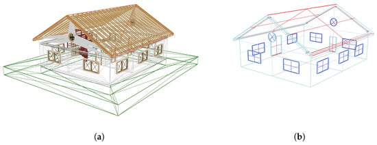
Figure 1. The difference between a building represented by a BIM model (a) and a 3D city model (b). It can be seen that the building is represented by distinct different elements in a BIM model. The building’s representation in a 3D city model is constructed out of a single shell comprising multiple surface types.

There is a large body of research on the conversion of BIM models to 3D city models (Section 2), but most methods in the literature tend to avoid applying complex geometric processing to the models. This keeps the methods simple but is also limiting what can be achieved. For instance, it is difficult or impossible for such a method to output models that are geometrically valid or fully conform to a particular standard (such as creating a closed shell representation as displayed in Figure 1b).

In this paper, we present our methodology (Section 3) to tackle the creation of building models at particular levels of detail (LoDs). LoD is a key feature of 3D city modelling standards that enables efficient and scalable creation, processing and use in applications [3]. Our method starts with detailed BIM models in the open Industry Foundation Classes (IFC) data model and abstracts them to nine different generalised output models that fit within the LoD frameworks in the open CityGML [4,5] and CityJSON [6,7] standards.

The selection of output LoDs has been created based on the goals of the Horizon Europe funded CHEK (Change Toolkit for Digital Building Permits) project. In this project, a toolkit has been developed to check new and renovated buildings (modelled in BIM) against urban regulations (e.g., maximum building height) by integrating the BIM models into the 3D city models. For this integration, abstractions of the BIM models need to be derived, containing the geometrical and semantic properties as needed for the regulations checking. This paper is a summary of the technical report of the BIM to Geo abstraction tool, which is available at https://research.tudelft.nl/en/publications/bim2geo-converter accessed on 26 November 2025.

Section 4 describes the implementation details of the method, which has been made into an open source prototype. Section 5 analyses the results of testing the prototype with a variety of IFC files. Section 6 contains the conclusions.

2. Related Work

2.1. 3D City Model LoD Abstraction Frameworks

The CityGML standard, in its versions up to 2.0 [4], introduced an abstraction framework consisting of five levels of detail (LoDs) ranging from LoD0 to LoD4. In the case of buildings, LoD0 is a 2.5D representation of the building’s footprint or roof area (roofprint), LoD1 is a prismatic blocks with flat roofs, LoD2 adds the building’s roof structures and surface semantics, LoD3 is a detailed architectural models of the building’s exterior, and LoD4 is a detailed architectural model that also includes the interior.

In CityGML version 3 [5], the abstraction framework was overhauled (Figure 2) in two main ways: (1) surface semantics can be included (or excluded) in any LoD, and (2) LoD4 was removed and interior geometries are now allowed in all LoDs, which includes floor plans for LoD0. As a result of the latter change, different LoDs can be used to represent both the exterior and interior features of a building.

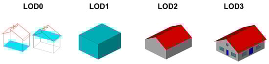
Figure 2. The four LoDs available in the CityGML 3.0 standard.

Considering the large gaps between LoDs, as well as the possibility of different interpretations of single LoDs in the standard, Biljecki et al. [6] proposed a finer-grained abstraction framework in which each LoD in the CityGML standard is split into four refined LoDs (Figure 3). Through this, an LoDx (where $0\le x\le 3$) in the original standard becomes four different levels of the form LoDx.y, where $0\le y\le 3$. This LoD framework is explicitly supported in the CityJSON standard [7].

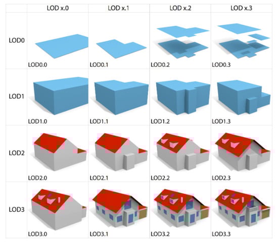
Figure 3. The 16 LoDs proposed by Biljecki et al. [6]. Surfaces with different colours have different semantics.

In this scheme, LoD0.x and 1.x follow a similar pattern, with 0.x modelling footprints and sometimes roof areas, and 1.x modelling volumes. LoD0.0 and 1.0 allow multiple buildings to be aggregated into a single geometry, LoD0.1 and 1.1 model buildings individually (without aggregation) with all their large parts, LoD0.2 and 1.2 also model smaller parts (e.g., alcoves) with roofs modelled/extruded at a single height, and LoD0.3 and 1.3 are similar but allow multiple roof surfaces at different heights. Note how LoD0.2 and 1.2, as well as 0.3 and 1.3, essentially encode the same information, as the missing walls in LoD0.x could be derived by extruding the roof surfaces down to ground level.

In LoD2.x, the different LoDs progressively add smaller elements that can be modelled. Starting from LoD2.0, which only models large building parts, LoD2.1 adds smaller building parts, LoD2.2 adds roof superstructures (e.g., dormers), and LoD2.3 adds explicitly modelled roof overhangs.

LoD3.x is characterised by explicitly modelled openings, e.g., windows and doors, but the abstraction scheme follows a different logic where the different LoDs do not have a strict increase in detail. LoD3.0 models detailed roof superstructures and their possible openings (e.g., skylights) but less detailed walls, whereas LoD3.1 is the opposite (detailed walls with openings but less detailed roofs) and models roof overhangs. These opposing modelling approaches reflect the elements that can be discerned from the two common data capture locations: from above (e.g., using satellite or aerial imagery and LiDAR) and from the ground (e.g., using terrestrial or car-mounted scanners). Finally, LoD3.2 models both detailed walls and roofs, and LoD3.3 incorporates finer details (e.g., window embrasures and awnings).

2.2. BIM to Geo Conversion

The problem of automatic BIM to Geo conversion has long been studied. Most early academic efforts focused on defining a mapping between equivalent BIM and Geo classes [8,9], or performed a conversion of some basic geometry types [10]. At roughly the same time, closed source software (e.g., FME and IFC Explorer) introduced basic functionality to convert from IFC to CityGML, but the methods used were not documented in the literature and the resulting files did not comply with the conventions and expectations of a typical CityGML file (e.g., containing non-overlapping and correctly classified semantic surfaces).

To our knowledge, the first well-documented effort to perform a BIM to Geo conversion was around the open source building information server BIMserver. Discussed in de Laat and van Berlo [11], it introduced two related pieces of work: the CityGML LoD4 export functionality of the software and a GeoBIM ADE of CityGML. As BIMserver can import IFC files, the export functionality could be used to perform an IFC to CityGML conversion, whereas the ADE allowed the storage of IFC semantics and properties in CityGML.

Later on, a few different methods which attempted to extract specific LoDs from BIM models were developed. For example, Donkers et al. [12] specifically targets the creation of CityGML LoD3 models. It uses a combination of semantic mapping of equivalent CityGML and IFC classes, geometric transformations based on constructive solid geometry to merge elements, and a process of geometric and semantic refinement to obtain missing surface semantics. There is an open implementation based on the Computational Geometry Algorithms Library (CGAL).

Similarly, Stouffs et al. [13] uses a triple graph grammar that defines a correspondence between equivalent elements in IFC and CityGML. Through this, object graphs for both IFC and CityGML are created and related to each other. The end result is a direct conversion of elements that should be geometrically equivalent to the input IFC model. The authors also define a CityGML Application Domain Extension (ADE) to improve the compatibility of CityGML with IFC, as well as the specificities of the Singaporean context of the study. The latter is described in more detail in Biljecki et al. [14].

A more recent representative example is described by Lam et al. [15], who target CityGML LoD4 specifically. Their method leverages the capabilities of existing software (FME 2023.1 and 3dcitydb) to perform the initial conversion, validates the results using the OWL/RDF semantic web technologies, and visualises the results using Cesium Ion and Unreal Engine 5.0.

A recent review of the scientific literature of IFC to CityGML conversion is contained in Liang and Tan [16], and Noardo et al. [2] provides a summary of the capabilities and limitations of other software for this purpose. In summary, while a few different pieces of software offer this functionality, the results are not ideal: output models are generally invalid, semantic mapping is difficult, and targeting specific LoDs is not realistic.

2.3. Abstraction Methods

In order to actually obtain 3D city models at specific LoDs from more detailed BIM models, applying an abstraction or generalisation method is necessary. Fan et al. [17] is an early example of an abstraction method to simplify building models in CityGML. They describe a few different techniques: extracting the outer envelope of approximately convex buildings, simplifying ground plans (useful for the bottom of building models), generalising façades, and substituting detailed windows for typified templates.

Deng et al. [18] proposed an instance-based method to create mapping rules between equivalent IFC and CityGML classes, which are formally stored in a reference ontology called the Semantic City Model. The study focuses on the transformation of coordinates and the creation of explicit geometries. Multiple LoDs can be generated from a BIM model by selecting or removing particular types, as well as by extracting the outer envelope of a building using ray casting.

Kang and Hong [19] uses a method that combines exterior envelope extraction and custom LoD mapping rules to extract multiple CityGML LoDs from a BIM model. The exterior envelope extraction uses a screen buffer to sample the surfaces that are visible from the exterior quickly, which can be implemented in a GPU.

Similarly, Zhou et al. [20] use a number of different observation points known to be in the exterior of a building to extract its outer envelope. As only the exterior surfaces of a building are visible from these observation points, this can be used to efficiently obtain these surfaces.

Ji et al. [21] use an ontology-based method to extract specific CityGML LoDs from an IFC file. Rule maps are used to convert coordinates (local to global), filter or extract geometries, and map the semantics of the different objects.

In sum, there is existing academic work to extract simplified 3D city models from BIM models, as well as to simplify existing 3D city models. Most of these methods tackle the creation of general-use useful shapes, such as exterior envelopes, whereas a few focus on the creation of specific CityGML LoDs. However, it is worth noting that even among the limited methods that attempt to extract specific LoDs, none addresses the creation of LoDs within the extended LoD framework of Biljecki et al. [6], and none offers a complete pipeline from BIM to Geo with an open implementation. Our methodology, presented in the following section, proposes a solution to this problem.

3. Methodology

The methods developed for the abstraction of BIM (IFC) models to Geo (CityJSON) models at different LoDs that form the BIM2Geo methodology developed in this research can be split into different steps.

Before the computation of the desired LoD abstraction output, our methodology always starts with a preprocessing step, which reduces the data’s complexity to ease the next steps. In this preprocess, the model’s placement is optimised, the objects required for the processes are selected, and complex objects (doors and windows) are simplified.

Secondly, a voxelisation step is required for every LoD except for LoD0.0 and 1.0. Here, the voxels that are used for the coarse filtering of data in most of the downstream abstraction processes are computed.

This is followed by a series of abstraction-specific processing steps. These are the processes where the actual abstracted shapes (i.e., geometries) are created. Depending on the required output LoD geometries, certain processing steps are executed while others are omitted. Roughly, the LoD abstraction methods can be grouped into five different levels. These levels are based on how much of the geometry of the input IFC model the methods rely on. The levels of geometric dependency and the individual LoDs generated are presented in Table 1. In addition to the standard LoDs described by Biljecki et al. [3], we consider one more useful LoD that consists of the roofing structure of LoD2.2, which we hereafter refer to as LoD0.4; see Figure 4. The IFC elements that the different methods use are shown in Figure 5.

Table 1. The five levels of geometry dependence of the different LoD abstractions. * Non-standard LoD.

level	Output	Based on BIM Model’s
low	LoD0.0 and LoD1.0 exterior	vertices
mid	LoD0.2, 0.3, and 0.4 * roof	roof geometry
	LoD1.2, 1.3 and 2.2 exterior
high	LoD0.2 and 0.3 storeys	selective outer shell
very high	LoD3.2 exterior	complete outer shell
interior	LoD0.2, 1.2, 2.2, and 3.2 interior	IfcSpaces

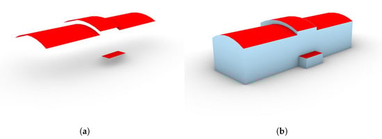
Figure 4. Example of LoD0.4 (a) which stores the roof surfaces of LoD2.2 (b) in a non-volumetric manner.

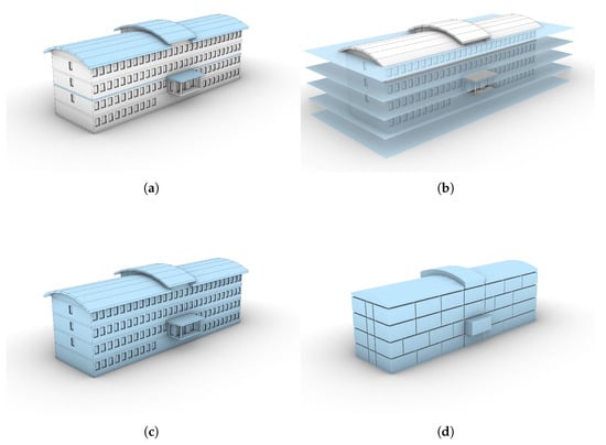
Figure 5. The elements relevant for the different abstraction methods. Low geometric dependent abstraction uses the vertices of the model. (a) Mid geometric dependent abstraction uses the roofing structure. (b) High geometric dependent abstraction uses the geometry at horizontal internals (the blue planes signify the horizontal sections taken). (c) Very high geometric dependent abstraction uses the complete outer shell. (d) Interior geometric dependent abstraction uses the IfcSpace objects.

A schematic overview of the methods and their relationships can be found in Figure 6. As this overview shows, some of the output LoDs are obtained by a mix of the five methods. For example, for a full LoD0.3 model, the LoD0.3 roof structure would be created via the mid geometric dependent abstraction methods, and the LoD0.3 storeys and footprint would be created via the high geometric dependent abstractions.

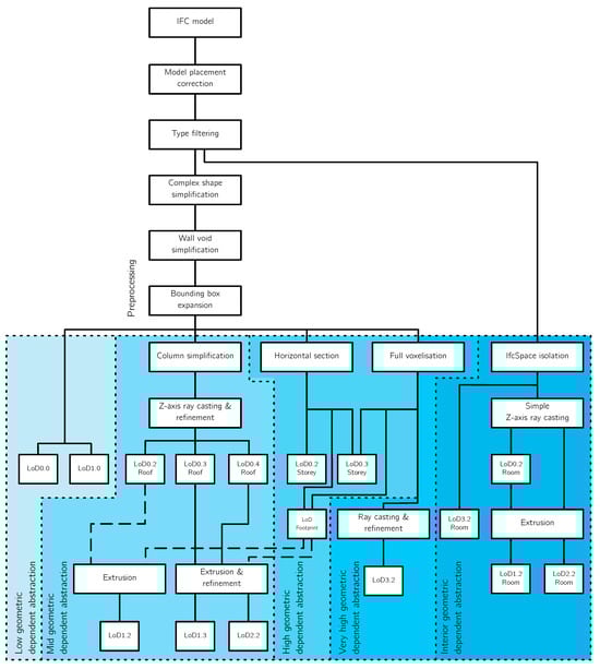
Figure 6. Flowchart to show the relationships of the different steps in the process (simplified). Non-standard LoDs are shown in grey. Optional connections based on the desired output refinement are shown in dashed lines.

3.1. Preprocessing

The preprocessing encompasses three different simplifications steps: the model placement is corrected, objects are filtered based on their IfcClass, and objects with complex geometries are simplified.

3.1.1. Correction of Model Placement

An IFC model can be placed in sub-optimal ways in its local coordinate system. Mostly, three unwanted situations can occur: a model is placed far away from its local coordinate system’s origin, a model is rotated in a way where it is not axis aligned to its local coordinate system’s axis, or both. These issues are fixed by computing translation and rotation vectors that place the model close to the coordinate system’s origin $(0,0,0)$ and align it to the local coordinate system’s axes.

3.1.2. Class Based Selection

The first and coarsest filtering step is the filtering based on IFC object class. For the abstraction of BIM models to GIS models, only space-dividing objects are required [22]. These objects represent physical/tangible geometries that play a role in the division of space. Examples are walls, floors, and roofs that encapsulate specific spaces and isolate the interior of the building from the exterior. The space-dividing objects are only utilized for the abstraction of the exterior of the building. The interior abstractions are based on the IfcSpace representations instead. Therefore, if interior spaces are to be abstracted and exported to CityJSON, the IfcSpace objects are also filtered.

3.1.3. Complex Object Abstraction

After the initial filtering step, the geometry of complex objects, i.e., IfcDoor and IfcWindow, is simplified. These objects often include many small details, such as hinges and grips, which are not relevant at a GIS scale and unnecessarily increase the complexity of subsequent abstraction steps.

Because doors and windows are often box-like in nature, they can be abstracted by replacing their geometry with an orientated smallest bounding box in full 3D space (using X, Y, and Z rotation); see Figure 7. However, not all IfcDoor and IfcWindow objects can be simplified using this box simplification, such as if a window has a triangular frame.

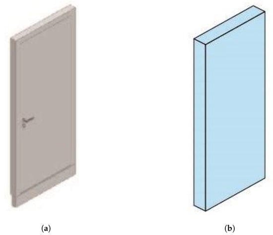
Figure 7. Simplification by bounding box creation. (a) A complex IfcDoor object. (b) The resulting bounding box that is used to replace the IfcDoor geometry. Image from [22].

Alternatively, a more drastic abstraction of windows and doors can be achieved by selectively applying subtractive elements. Doors and windows are often placed in openings, which are modelled with IfcOpeningElement or IfcFeatureElementSubtraction objects. If these subtractive elements are not applied (Figure 8), the windows and doors that were placed inside of these openings can be discarded without creating a hole between the interior and exterior.

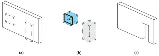
Figure 8. Selectively applying subtractive shapes in an IfcWall object. (a) A wall with subtractive objects. (b) The objects encapsulated by these subtractive objects. The grey void has no nested objects while the blue void has a nested IfcWindow object. (c) Only the subtractive objects with no internal objects is applied, resulting in the simplified wall geometry. Image from [22].

3.2. Voxelisation

For mid, high, or very high geometric dependent abstraction processes, a voxel grid is created. The use of the voxels is primarily coarse filtering of IfcObjects to speed up computation, although in the high and very high geometric dependent abstraction processes, it also fulfils a different role. If mid geometric dependent abstraction is to be executed, the voxel grid is populated with voxel columns. If high or very high geometric dependent abstraction is selected, the voxel grid will be populated with full voxelisation.

Column voxelisation is the result of “growing” voxels vertically in a column-like shape; see Figure 9. For the full voxelisation, each voxel is independently tested for intersection with a mesh representation of any of the space-dividing objects. After the intersection test has been executed for all voxels, the exterior space can be grown from one of the voxels that are at the edge of the domain.

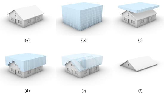
Figure 9. Column voxelisation. (a) Starting IFC model. (b) Full voxel grid. (c) Top slice of voxels from which the growing is started. (d) Elongated columns that are grown up until they hit geometry. (e) An isolated voxel with the wireframe of the geometry it intersects with highlighted. (f) The isolated geometry of the model that intersects with the voxel columns. Note that from (c) onward the outer ring of columns has been hidden for clarity.

As noted by van der Vaart et al. [23] the “ideal” voxel size depends on the size and nature of the model that has to be voxelised. A too large voxel size might miss detail required for any of the downstream applications, while a too small voxel size will slow down the subsequent processes and reduce robustness. Therefore, the voxel size can be selected by the user so that it can be fine-tuned to fit the model that is to be processed. In general, a voxel size between 0.1 to 0.4 m functions well on most models.

3.3. Low Geometric Dependent Abstraction

The low geometric dependent abstraction processing extracts the LoD envelopes that are primarily based on the model’s vertices (LoD0.0 and 1.0 exterior). The LoD0.0 representation can consist of two faces: a face representing the roof outline and a face representing footprint outline. If the LoD0.0 roof outline is desired, the face representing the roof outline is created based on a tightly encapsulating bounding box surrounding all the space-dividing objects. The top surface of this bounding box is isolated and stored as an independent object in the output file. The surface type is set to RoofSurface. If no footprint outline is desired, the roof outline surface is placed at the footprint height instead of at the top height. Instead of the RoofSurface surface type, this surface has the custom surface type +ProjectedRoofOutline. If the LoD0.0 footprint outline is desired, a new bounding box has to be created. The tightly encapsulating bounding box surrounds all objects, while the footprint in theory can be smaller. The footprint outline LoD0.0 surface is based on the bounding box of all the objects that are placed at, or intersect with, the footprint level $\pm 0.15$ m. The lower vertical surface of this bounding box is isolated, placed at the footprint height, and stored as an independent object in the output file. The surface type is set to GroundSurface.

The LoD1.0 representation is a copy of the shape of the tightly encapsulating bounding box surrounding all the space-dividing objects. The type of the four surfaces of this box that have a normal with a Z-component of close to 0 are set to WallSurface. Of the two remaining surfaces, the type of the surface with the highest Z-value is set as RoofSurface. The type of the other surface is set as GroundSurface.

3.4. Mid Geometric Dependent Abstraction

The mid geometric dependent abstraction extracts LoD envelopes and projections that are primarily based on the model’s roofing structure (LoD 0.2, 0.3, and 0.4 roof structures and 1.2, 1.3, and 2.2 exterior). The roof related elements are isolated in two steps: coarse filtering with column voxelisation and fine filtering via ray casting in Z-direction; see Figure 9 and Figure 10.

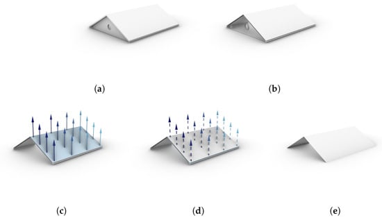
Figure 10. Surface filtering and ray casting to isolate the surfaces that are part of the roof structure. (a) The surface collection collected via the column voxelisation. (b) The surfaces are filtered by eliminating the surfaces with normal $Z=0$. (c,d) An isolated situation of the ray casting process of the two viewer facing roof surfaces. The top surface in (c) has at least one non-intersecting ray (solid colour arrow). The bottom surface in (d) has no non-intersecting ray (dotted arrow). (e) Final result.

3.4.1. Filtering of Surfaces

The objects collected with the help of the column voxelisation are assumed to have at least one surface that could play a role in the construction of LoD0.2, 0.3, 1.2, 1.3, and 2.2. The unique objects that are intersected with and their surfaces are selected. The selected objects’ surfaces are further filtered via a ray casting process where the rays are cast from each surface upwards parallel to the Z-axis.

This is followed by a polyhedral surface approximation, as an IFC file supports both implicit and explicit geometry while CityJSON only supports explicit geometry.

3.4.2. Creating Surface Based Abstractions

To construct the LoD0.2 roof abstraction, the surfaces identified as part of the visible roof structure are all projected to the $XY$-plane (Z = 0) and merged into a single surface: the projected roof outline. If footprint extraction is to be executed/exported, which can be generated by the high dependent abstraction method (see Section 3.5), the roof outline surface is translated to the max height of the building. The surface type is set to RoofSurface. If no footprint extraction is to be executed/exported, the projected roof outline is stored at the ground level of the model. In this case, the surface type of the surface is set to +ProjectedRoofOutline.

To construct the LoD0.3 roof abstraction (i.e., with varying height in case of significant height jumps), the surfaces identified as part of the visible roof structure are grouped and flattened; see Figure 11. Then, the surfaces are trimmed by extruding the roof surfaces downwards to the lowest height of the input model to form solids, which are used to split the flattened isolated roof surfaces.

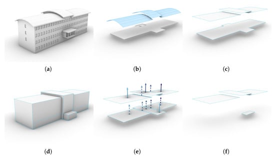
Figure 11. The steps of the LoD0.3 roof abstraction. (a) The model used. (b) The fine filtered roof surfaces (3 groups) that were isolated with the help of column voxelisation and ray casting. (c) These groups are flattened. (d) The surfaces are extruded to ground floor level, and each original un-extruded surface is split with the extruded shapes that intersect it. (e) The split surfaces are filtered with the help of a ray casting process, solid arrows do not intersect, dotted ones do intersect. (f) The resulting LoD0.3 surfaces.

To create the LoD0.4 roof surfaces, all the steps of LoD0.3 are followed except for the grouping and flattening of the shapes. The surface types of both the LoD0.3 and 0.4 roof surfaces are set to RoofSurface.

3.4.3. Creating Volumetric Abstractions

To construct the LoD1.2 exterior abstraction, the LoD0.2 roof outline surfaces are projected to the $XY$ plane (Z = 0) and extruded upwards to the max height of the building.

The same logic for the surface semantics that is applied for the LoD1.0 shape (see Section 3.3) is applied here. The type of the surfaces that have a normal with a Z-component of close to 0 are set to WallSurface. Of the two remaining surfaces, the type of the top surface is set as RoofSurface and the type of the lower surface as GroundSurface.

The constructions of the LoD1.3 and 2.2 exterior abstraction are closely related to each other, but the LoD1.3 reconstruction uses the LoD0.3 roof structure as a starting point and LoD2.2 uses the LoD0.4 roof structure. Each of the starting surfaces (either the LoD0.3 or LoD0.4) are extruded downwards to the ground level and merged into a single solid.

A similar process for surface semantics that is applied for the LoD1.0 and LoD1.2 shape is applied for LoD1.3 and 2.2. The type of the surfaces that have a normal with a Z-component of close to 0 are set to WallSurface. The type of the surfaces that are at the footprint height are set to GroundSurface. The type of the remaining surfaces are set to RoofSurface.

If desired, the LoD1.2, 1.3, and 2.2 exterior abstractions can be restricted by the outline of the model’s footprint. This does, however, require the footprint to be generated, which is a more complex process that relies on more parts of the IFC model’s geometry; see Section 3.5.

For the LoD1.2 footprint-restricted exterior abstraction, the footprint can be extruded upwards to the building’s max height. For the LoD1.3 and 2.2 footprint-restricted exterior abstraction, the roofing surfaces that overhang over the footprint can be trimmed down before being used for extrusion; see Figure 12. The rest of the processes for creating both LoD1.3 and 2.2 remain exactly the same.

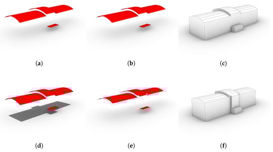
Figure 12. The difference between roof-structure-based LoD2.2 creation (a–c) and footprint-restricted LoD2.2 creation (d–f). The column (a,d) shows the input geometry required. The column (b,e) shows the faces used for downward extrusion in red. It can be seen that some surfaces are not used for footprint-based extraction (in white); these are parts of the roof surfaces that extend over the footprint. The column (c,f) shows the resulting shapes.

When the footprint-based extraction is used, the LoD0.2, 0.3, and 0.4 roof surfaces can differ from the LoD1.2, 1.3, and 2.2 roof surfaces, respectively. The LoD0.2, 0.3, and 0.4 roof surfaces remain untrimmed, so when overhang is present over the footprint, this will be reflected by these roof surfaces. The footprint-based LoD1.2, 1.3, and 2.2 roof surfaces can possibly cover a smaller area in comparison.

3.5. High Geometric Dependent Abstraction

The high geometric dependent abstraction processing extracts elements that are based on the model’s outer shell (LoD0.2 and 0.3 storey representation and the LoD0.2 and 0.3 footprint). Unlike the very high geometric dependent abstraction processes (see Section 3.6), these processes only sample the outer shell at certain intervals: at the storey heights and at the building’s footprint heights.

The LoD0.2 and 0.3 storey abstraction rules are not well described in existing documentation. Therefore, we tried to apply the rules defined for the exterior to the interior storeys. For LoD0.2, a storey is represented as a horizontal surface (or group of surfaces) representing all the objects in a building at a certain storey elevation. This surface (or group of surfaces) will span the entire building at a single height. This loosely resembles the single top surface logic of the exterior LoD0.2 roof surface. For LoD0.3, a storey is represented as a horizontal surface (group) representing all the objects at a certain storey elevation that are related to that storey. This surface (group) can span only a part of the building at a single height. Depending on how the IFC model has been constructed, this resembles the multiple horizontal flat plane LoD0.3 logic. Additionally, we decided to add extra functionality to the LoD0.3 storeys by expanding its stored surface semantics.

Similarly to the storey abstraction rules, the footprint abstraction rules of LoD0.2 and 0.3 are also not well described in documentation. Due to time constraints, we chose to create the same shape for both: a horizontal surface (or group of surfaces) representing all the objects in a building at a certain user submitted footprint elevation.

3.5.1. Simple Approach for Storey Abstraction

This abstraction method leads to an LoD0.2 storey representation by taking a horizontal section through all the input model’s space-dividing objects at each of the storeys’ heights. These heights are found by taking the elevation attribute of the IfcBuildingStorey objects. If modelled properly, this height should represent the elevation of the top of the construction slab of a storey. If multiple storeys are present with the same or similar elevation values they are grouped together and handled as if they are a single storey object. This can occur when a model is constructed from multiple IFC files.

The used surface type for all the created surfaces is FloorSurface. The attributes of the IfcBuildingStorey object(s) at that elevation can be copied to the CityJSON storey object. Each of these CityJSON objects has a parent/child relationship to the main building’s CityJSON object to keep the clear structure in the reconstructed model.

3.5.2. Complex Approach for Storey Abstraction

The storeys of the LoD0.3 abstraction are created in a similar manner as LoD0.2 but with two major differences. Firstly, the horizontal section at the storey elevation splits only the objects that are related to that IfcBuildingStorey object or group of IfcBuildingStorey objects at the storey elevation. This allows the accurate inclusion of half or split storey elevations across a building model, but requires the IFC model to have the correct objects bound to the storey surfaces. Secondly, during the process, the surfaces are divided based on if they are interior or exterior. This makes it possible to isolate balconies and parts of the (flat) roof structure and to not include these outdoor parts in downstream analysis, if, for example, only the interior is required. The interior/exterior distinction is made with the help of the voxel grid. For every surface, it is tested if the voxels above it are representing the exterior. If any of the voxels is representing the exterior, the surface is considered exterior. Otherwise, the surface is considered interior.

Both the interior and exterior surfaces can be stored in the same BuildingStorey CityJSON city object representing the group of storeys at that elevation. The used surface type is FloorSurface for the interior surfaces and OuterFloorSurface for the exterior surfaces. As with the LoD0.2 storeys, the attributes of the IfcBuildingStorey object(s) at that elevation can be copied to the city object. Each of these CityJSON objects has a parent/child relationship to the main building’s CityJSON object to keep the clear structure in the abstracted model.

3.5.3. Footprint Abstraction

The footprint abstraction method (LoD0.2 and LoD0.3) follows a very similar approach to the LoD0.2 storey abstraction. Instead of the storey’s elevation, the footprint elevation is taken as the height of the horizontal section. The final LoD0.2 surface is further refined by selectively removing inner loops, as certain voids, such as elevator or staircase shafts, are not important for the (outdoor) footprint geometry. The voids are filtered with the help of the voxel grid. For every inner ring’s void area it is tested if the voxels above it are representing the interior. If any of the voxels is representing the interior, the ring is ignored.

The surfaces representing the footprint are stored in the same CityJSON object in the CityJSON file as the roof abstractions. The footprint shape is considered to be exterior. The type of the surface is set as GroundSurface.

3.6. Very High Geometric Dependent Abstraction

The very high geometric dependent abstraction processing extracts LoD abstractions that are based on the complete model’s outer shell, including windows and doors (LoD3.2 exterior). It is the highest dependent abstraction method and requires well-made models to function properly. The creation of the LoD3.2 abstraction can be split into three main processes: surface filtering, surface refinement, and the fetching process of the attribute data. A visual example of the complete process can be seen in Figure 13.

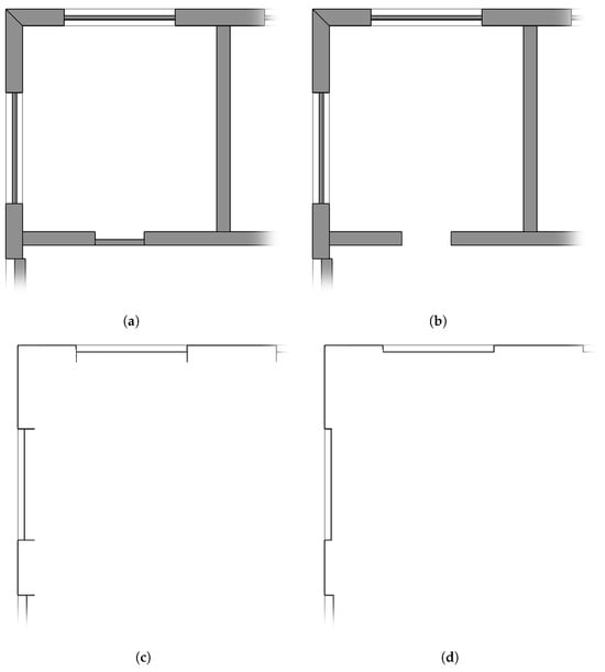
Figure 13. The steps of LoD3.2 abstraction. (a) The starting situation after the IFC class filtering and complex shape simplification. (b) The objects that are close to the exterior of the building model are isolated by using the intersecting voxels that neighbour an exterior void voxel. (c) The fully inner surfaces are filtered out by voxel-assisted ray casting. (d) The surfaces are split and again filtered out by voxel-assisted ray casting.

3.6.1. Surface Filtering

The aim is to isolate the surfaces that play a role in the construction of the exterior shell of the building. This filtering is performed with the help of a voxel-assisted ray casting process. During the voxelisation process, described in Section 3.2, the voxel objects store data related to their intersections. With this information, a coarse filtering of the objects can be made. The intersecting voxels that have one, or more, neighbouring voxels that are non-intersecting and external are assumed to represent the exterior shell of the building. The IFC objects with which these filtered voxels intersect are assumed to have at least a single surface that is part of the exterior shell. The unique intersecting objects of this group of voxels are collected and used in the ray casting process.

The surfaces of the collected objects are filtered with the help of the voxel-assisted ray casting process. This is performed by populating each surface with a point grid. From these points, rays are cast to the centres of the surrounding non-intersecting exterior voxels. For every point on the surface, the exterior voxels that fall within 1.5 times of the voxel size are selected as ray target points. Every ray is tested for an intersection with any of the surrounding meshed surfaces (except the surface from which it originates). If the ray intersects with anything, it is considered a hidden ray. If the surface has at least one ray that is not hidden, it is considered of importance and collected for further processing.

3.6.2. Surface Refinement

The surfaces that were collected are at least partially exterior. However, these surfaces can still have parts that are interior; see Figure 13. These interior parts need to be eliminated to be able to create a closed outer shell. During this surface refinement step, the surfaces are split and filtered.

The surfaces are split by the surrounding surfaces that they touch. After all the surfaces are split, they comprise a new pool of surfaces that are either completely exterior or interior. To detect if the surface is visible, another voxel-assisted ray cast process is used. This is similar to that described in Section 3.6.1 but only utilises a single point from which a ray is cast. The resulting surfaces are considered to be completely visible. The surfaces that are considered to be completely visible can be merged based on their surface type. Due to the complexity of the types, three distinctions are made: doors, windows, and others. Surfaces that touch, have a parallel normal, and are part of the same type group can be merged into a single surface.

3.6.3. Acquiring Attribute Data

To be able to merge the surfaces based on their type and to correctly store them as CityJSON surfaces, attribute data is required. In most cases, the IFC object class is utilized, e.g., IfcWall objects are walls and IfcRoof objects are roofs. Table 2 shows a full overview of the BIM to GIS types. However, in certain cases this is not enough. For example, windows and doors can also be part of IfcCurtainWall objects; see Figure 14. If a window is present in a curtain wall, it is often modelled as an IfcPlate object. Consequently, a method had to be developed to detect if an IfcPlate object is a window.

Table 2. The relationship between IFC types and CityJSON surface types.

IfcClass	CityJSON Type
IfcDoor	All surfaces: Door
IfcWindow	All surfaces: Window
IfcPlate with glass like material	All surfaces: Window
IfcSlab	If below ground level:
	Horizontal: FloorSurface
	Other faces: WallSurface
	If Above ground level:
	Horizontal: RoofSurface
	Other faces: WallSurface
Other classes	WallSurface

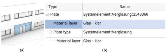
Figure 14. (a) The window/door structure of the main entrance of the digital HUB model (its windows highlighted in blue) is modelled as an IfcCurtainWall where the windows are IfcPlate class objects. (b) The model is modelled by a German party, so relying on the material name, which is expected to be English, would not work.

The most reliable way of detecting windows that are nested in IfcCurtainWall objects is by the material rendering properties which are stored in the IfcSurfaceStyleRendering class. This rendering class has a transparency attribute that ranges from 0 to 1. If the transparency is larger than 0.25, the surface is considered to be a window surface.

Relying on the IfcMaterial object’s name attribute is an alternative option. If the material represents glass, the words “glass” or “glazed” are often part of the material’s name. However, this is not always the case. For example, if a language other than English is used, the words would have to be translated; see Figure 14.

The way of detecting the windows passes through all the three options. First, the class type is used. If the type is IfcCurtainWall or IfcPlate, the IfcMaterial class’s name attribute is searched for. If this name contains the words “glass” or “glazed", the surface is typed as a window. If this is not the case, the final option is followed and the IfcSurfaceStyleRendering class properties are used.

3.7. Interior Geometric Dependent Abstraction

Interior extraction methods are defined for LoD0.2, 1.2, 2.2, and 3.2 abstractions, where each room in the input model is represented by a unique shape. LoD0.2 uses only the ceiling outline, while LoD1.2–3.2 provide full volumetric abstractions.

The abstracted shapes representing the interior rooms are based on the IfcSpace objects, which are modelled similarly in the IFC model to their abstracted GIS representations will be; see Figure 15. They are both modelled as a shell representing the transition between tangible geometry and interior void, which makes it a fairly easy process to transition from IFC to CityJSON. However, if there is no IfcSpace data present or if the geometry representation is incorrect, the abstracted shape will also be missing or incorrect.

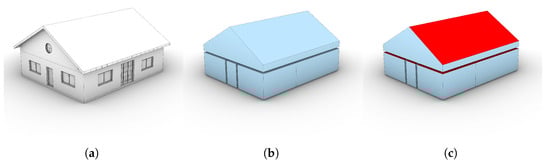
Figure 15. Comparison between the IFC interior space objects (b) and the CityJSON interior space objects (c) of the FZK_haus model (a). Aside from the surface types, the geometric shapes of the IFC spaces and CityJSON spaces are identical.

To create the LoD0.2, 1.2, and 2.2 interior abstractions, the ceiling structure of the IfcSpace has to be isolated; see Figure 16. This process is similar to the roof structure detection described in Section 3.4.1.

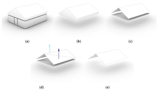
Figure 16. The steps that are taken for the ceiling detection. (a) The starting shapes are the IfcSpace objects. (b) For a more clear visual, one room is isolated. (c) The vertical faces are discarded. (d) A ray is cast from the surface to test for intersection. (e) The surfaces from which a non-intersecting ray is cast are collected; these are the surfaces representing the ceiling structure.

For LoD0.2, the ceiling surfaces are projected flat, merged, and translated to the Z height of the lowest point of the original IfcSpace object. Similarly to the LoD0.2 roof outline of the exterior shell, this surface has the type of a top surface. In this case, that is the +ProjectedCeilingOutline type.

To create the LoD1.2 abstraction, the flattened merged surface that has been created for LoD0.2 is extruded upwards to the top height of the IfcSpace object’s geometry. The type of the surfaces that have a normal with a Z-component of close to 0 are set to InteriorWallSurface. Of the two surfaces that are left, the type of the top surface is set to CeilingSurface and the type of the bottom one to FloorSurface.

LoD2.2 uses the un-flattened ceiling surfaces. These are extruded downwards to the lowest height of the original IfcSpace object. The type of the resulting shape’s surfaces that have a normal with a Z-component of close to 0 are set to InteriorWallSurface. The type of the lowest of the remaining untyped surfaces is set to FloorSurface. The type of the rest of the surfaces is set to CeilingSurface.

The LoD3.2 abstraction shapes for the interior are not actual abstractions. They are almost 1:1 conversions of the IfcSpace geometry. The only difference is that IFC supports implicit geometry while CityJSON only supports explicit geometry. If implicit geometry is used to represent the surfaces modelling the room, the surfaces are approximated by polyhedral surface approximation.

Similarly to that performed for the LoD1.2 and 2.2 abstractions, surfaces that have a normal with a Z-component of close to 0 are walls. However, angled walls can occur in LoD3.2. Consequently, there can be a case where a wall has a normal with a Z-component that is not close to 0. To be able to correctly detect those surfaces as walls, an extra rule is added. If a surface normal falls within a 20 degree angle of a horizontal plane, the surface is considered a wall.

Unlike the interior abstraction spaces of LoD1.2 and 2.2, the LoD3.2 shape can have multiple surfaces representing the floor. To detect the floor surfaces, a ray cast is made from each surface upwards along the Z-axis. If it intersects with any other surface, except itself, it is considered a floor surface. All the remaining surfaces are marked as ceiling surface.

4. Implementation Details

4.1. Bim2geo Application

The methods described in Section 3 were implemented in an open source software application called the IfcEnvelopeExtractor. This allows us to test the viability of these methods in an automated manner. The IfcEnvelopeExtractor is a cross-platform (Windows and Linux) console application that takes an IFC model as input and automatically converts it to a CityGML/CityJSON file with minimal user assistance. Precompiled Windows or Ubuntu Linux versions can be acquired from the application’s GitHub page: https://github.com/tudelft3d/IFC_BuildingEnvExtractor accessed on 26 November 2025. The utilized version for this research is V0.2.6.

The application is C++ based and utilizes the IfcOpenShell 0.7 and OCCT 7.5.3 libraries for accessing the BIM data and processing the geometry. In conjunction with the IfcEnvelopeExtractor, the C++ open source library CJT was developed. CJT enables editing of CityGML/CityJSON files and the conversion of OCCT geometry to CityGML/CityJSON.

4.2. Used Models

The models tested cover a wide range of building types, from simple single houses to multistorey offices, including CHEK project use cases (Table 3, Figure 17). Two out of the six evaluated models required editing to meet input requirements of the methods and the IfcEnvelopeExtractor. As objects are selected by type, issues arose when models used incorrect types, e.g., a road in the FM_ARC_DigitalHub model was classified as an IfcSlab. Such cases were corrected by changing or removing the object type.

Table 3. Summary of the models used to test performance.

File Name	Source	IFC Version	Object Count	Storeys	$\mathit{X},\mathit{Y},\mathit{Z}$ Size (m,m,m)
AC20-FZK-Haus	IAI/KIT	IFC4	102	2	15.0, 13.0, 6.5
AC20-Institute-Var-2	IAI/KIT	IFC4	896	5	64.4, 42.2, 15.4
FM_ARC_DigitalHub	RWTH Aachen	IFC4	775	3	64.3, 35.6, 12.1
PRAHA_GO_V5	CHEK	IFC4	3588	7	91.4, 61.2, 26.1
Demo_Lisbon_2025	CHEK	IFC4	591	7	33.3, 11.4, 19.4
Demo_Ascoli Piceno_v2	CHEK	IFC4	3040	8	61.6, 57.7, 22.1

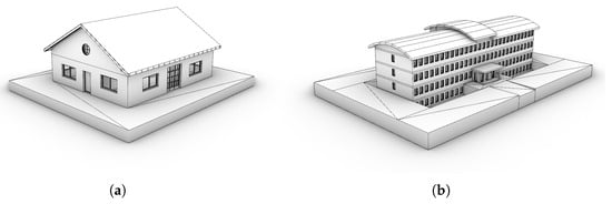
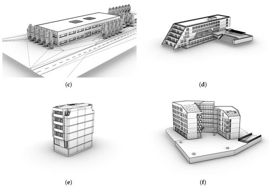
Figure 17. The different models that are used to evaluate the performance of the developed methods. (a) AC20-FZK-Haus model, (b) AC20-Institute-Var-2, (c) FM_ARC_DigitalHub, (d) PRAHA_GO_V5, (e) Demo_Lisbon_2025, (f) Demo_Ascoli Piceno_v2. The figures representing these models are not to the same scale.

5. Results, Evaluation, and Discussion

5.1. Geometric Accuracy

We assessed geometric accuracy by visually comparing the input IFC models with their abstractions and checking whether volumetric outputs formed closed shapes and do not have any extra elements. Instead of a binary evaluation, we used three scores: 1 (correct/as expected), 0.5 (minor issues but still usable), and 0 (major issues preventing GIS analysis). The results (see Table 4 and Table 5) show that non-volumetric abstractions perform very well, while volumetric accuracy decreases with complexity: LoD1.0 and 1.2 scored high, but LoD1.3 and complex shapes scored lower. Footprint-restricted abstractions followed the same trend. All interior abstractions scored 1 across 2D, 2.5D, and 3D outputs.

Table 4. The success rate of the exterior shell extraction. * Output differs per execution.

File Name	LoD0.0	LoD0.2	LoD0.3	LoD0.4	LoD1.0	LoD1.2	LoD1.3	LoD2.2	LoD3.2
AC20-FZK-Haus	1	1	1	1	1	1	1	1	0.5
AC20-Institute-Var-2	1	1	1	1	1	1	1	1	1
FM_ARC_DigitalHub	1	1	1	1	1	1	1	1	0.5
PRAHA_GO_V5	1	1	1	0–1 *	1	1	1	0.5–1 *	0
Demo_Lisbon_2025	1	1	1	1	1	1	0.5	0.5	0.5
Demo_Ascoli Piceno_v2	1	1	1	1	1	1	0.5	0.5	0

Table 5. The success rate of the footprint-restricted exterior shell extraction.

File Name	LoD1.2	LoD1.3	LoD2.2
AC20-FZK-Haus	1	1	1
AC20-Institute-Var-2	1	1	1
FM_ARC_DigitalHub	1	1	1
PRAHA_GO_V5	1	1	0.5
Demo_Lisbon_2025	1	1	0.5
Demo_Ascoli Piceno_v2	1	0.5	0.5

5.1.1. Propagation of IFC-Model-Related Issues

Even models rated 1 may be unusable if the input IFC is faulty, as errors in the input file propagate through the IfcEnvelopeExtractor. Demo_Ascoli Piceno_v2 illustrates two different occurrences of this. First, open connections between the building’s exterior and the underground parking and staircase shafts prevent a clear interior–exterior distinction, so these spaces are classified as exterior, which is consistent with geometry but not user expectations. This can be noted across several LoDs (LoD0.2 and 0.3 footprints, LoD0.3 storeys, footprint-restricted LoD1.2, 1.3, and 2.2, and LoD3.2 exterior). Second, facade gaps (≥1 cm) due to modelling errors create issues in high and very high geometry-dependent abstractions (LoD0.3 and 3.2).

5.1.2. Tolerances/Precision

Volumetric abstractions face two issues: incorrect vertical face elimination in LoD1.3 and 2.2, and faulty surface trimming in LoD3.2, both linked to tolerances in IFC models and Boolean operations in the tool. The tool applies a tolerance of 0.001 mm (1 × 10^$-6$ m), which exceeds the modelling accuracy typically achieved in practice. While such small gaps are irrelevant in most BIM contexts, they affect the IfcEnvelopeExtractor. For example, in Demo_Lisbon_2025 and Demo_Ascoli Piceno_v2, minor gaps in roof structures prevented vertical faces from aligning, leaving remnant faces and blocking the creation of closed solids.

As shown in Table 4, the Demo_Lisbon_2025 and Demo_Ascoli Piceno_v2 models scored perfectly for LoD0.3 and 0.4 despite small gaps in the roofing structure, as these are below the GIS precision of 1 mm. However, overly strict tolerances cause trimming errors in nearly all LoD3.2 abstractions. Even in simple cases (e.g., AC20-FZK-Haus), untrimmed surfaces prevent models from being true solids, leaving watertight but invalid geometries (Figure 18). These errors often occur around windows, doors, and curtain walls, though simplifying complex objects can reduce their frequency.

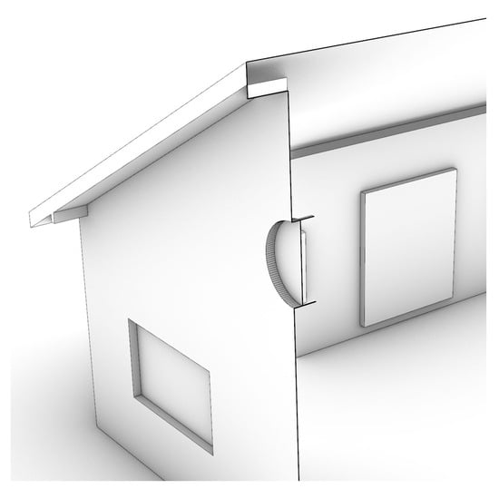
Figure 18. A section of the LoD3.2 abstraction of the AC20-FZK-Haus model that shows some of the incorrectly trimmed surfaces at the round window.

PRAHA_GO_V5 and Demo_Ascoli Piceno_v2 show poor LoD3.2 results, with incorrect trimming and missing surfaces. Although missing surfaces are a different issue, they stem from the same cause: faulty trimming. During the second ray-casting step (Section 3.6.2), split surfaces are assumed to be entirely interior or exterior. If the split is incorrect, a surface can be both, and its classification then depends on the ray origin, leading to missing or incorrect geometry.

5.2. Semantic Accuracy

We visually evaluate the surface types of each LoD abstraction to check if their type adheres to the description in the CityGML3.0 standard [5]. The tests showed that the surface types of all abstractions are as expected when compared to the CityGML 3.0 feature type documentation. The success rate of both the interior and exterior abstractions show that, even though the way that the surface types are determined is very simple, they are also accurate. Even on models that were not true solids, such as the Demo_Lisbon_2025 model, the surface types could still be accurately determined. Note that the surfaces that were incorrectly modelled were not included here, as these surfaces are not supposed to be there.

Even though the surface types were technically correct in the FM_ARC_DigitalHub and Demo_Lisbon_2025 abstracted models, these models have windows that are part of the roofing structure. Due to the simplicity of the rules that are used to determine the surface types, these were not classified as windows in the abstracted LoD1.3 and 2.2 shapes. LoD1.3 officially requires no surface types and LoD2.2 does not require the surface types that signify if a surface is a window or a door. However, the value of the models could be enlarged if window surfaces that are part of the roof structure can be identified as such.

5.3. Model Complexity

We compare the size of the different output files with the original input IFC file size. Table 6 compares the size of a 1:1 converted .obj file, the combined CityJSON abstraction containing the nine abstracted representations of the model (LoD0.0, 0.2, 0.3, 0.4, 1.0, 1.2, 1.3, 2.2, and 3.2 interior and exterior), and the LoD3.2 CityJSON abstraction to the original file. The 1:1 .obj file was added to this evaluation to include the file size of the input model with all explicit geometry. Similar to .obj, CityJSON only allows explicit geometry, while IFC also allows implicit geometry. This .obj model/file is also used for the other evaluations in this section.

Table 6. Comparison of the file size of the 1:1 OBJ conversion, the combined output GIS file, and the output GIS file containing LoD3.2 only to the input IFC file. All the files contain both interior and exterior abstractions. * This output file contains LoD0.0, 0.2, 0.3, 0.4, 1.0, 1.2, 1.3, 2.2, and 3.2.

File Name	OBJ File Size (%)	CityJSON File Size * (%)	CityJSON LoD3.2 File Size (%)
AC20-FZK-Haus	14.43	0.43	0.39
AC20-Institute-Var-2	39.63	8.71	8.06
FM_ARC_DigitalHub	303.70	1.35	0.78
PRAHA_GO_V5	3751.33	7.77	7.11
Demo_Lisbon_2025	548.52	1.26	0.65
Demo_Ascoli Piceno_v2	800.52	4.82	2.19
Average	909.69	4.05	3.20

This is followed by a comparison of the polygon count. Table 7 compares the number of triangles of the exterior abstractions with the 1:1 .obj conversion of the IFC model. To compute the number of triangles of the CityJSON abstractions, the shapes were triangulated using Rhino3D.

Table 7. Comparison of the number of triangles compared to the 1:1 OBJ representation of the exterior geometry in the IFC file. Note that this table is in per-thousand/per-mille and not percentages. * Faulty abstractions (<0.5).

	Triangle Count per-1000 (‰)
File Name	LoD0.2	LoD0.3	LoD0.4	LoD1.2	LoD1.3	LoD2.2	LoD3.2
AC20-FZK-Haus	0.19	0.19	0.27	0.56	0.56	0.74	65.53
AC20-Institute-Var-2	0.47	0.42	1.27	1.04	1.23	3.49	85.35
FM_ARC_DigitalHub	0.09	1.25	1.25	1.04	2.39	2.39	9.45
PRAHA_GO_V5	0.04	0.22	0.43	0.04	0.43	0.68	3.27 *
Demo_Lisbon_2025	0.17	0.72	1.01	0.22	1.02	3.23	6.54
Demo_Ascoli Piceno_v2	0.26	0.40	1.53	0.15	0.54	6.77	37.82 *
Average	0.20	0.53	0.96	0.34	1.03	2.71	34.66

Finally we compare the different complex object simplification processes. Table 8 compares the three different approaches to simplifying IfcWindow and IfcDoor objects to the original triangular polygon count.

Table 8. The effect of the complex shape simplification functions on the final triangle count. The full LoD3.2 has no complex shape simplification applied, the normal LoD3.2 has only bounding box simplification applied, and the simple LoD3.2 has bounding box and selective void simplification applied. This is just a comparison of the geometry. LoD3.2 is the outer shell only. * Faulty abstractions (<0.5).

File Name	Full LoD3.2 (%)	Normal LoD3.2 (%)	Simple LoD3.2 (%)
AC20-FZK-Haus	17.45 *	6.55	0.61
AC20-Institute-Var-2	24.42	8.53	0.76
FM_ARC_DigitalHub	- *	0.95	0.30
PRAHA_GO_V5	4.54 *	0.33 *	0.33 *
Demo_Lisbon_2025	23.45 *	0.68	0.68
Demo_Ascoli Piceno_v2	77.92 *	3.78 *	3.67 *

5.3.1. File Size

The file size evaluation (Table 6) shows a significant reduction from IFC to CityJSON. Even the combination file, containing nine abstractions, is much smaller than the input model. On average, output files are 4% of the original IFC size, with LoD3.2 files averaging only 3% while still retaining considerable detail.

The file size reduction results from multiple factors, with shape abstraction being assumed the most significant: simpler geometry requires less storage. Other contributors include eliminated semantic data, differences in file encoding, and the geometry storage method.

During abstraction, semantic data is reduced: only selected attributes are copied to the GIS file. For exteriors, IfcBuilding, IfcDoor, and IfcWindow attributes are retained (only IfcBuilding for LoD < 3.2), while for interiors, only IfcRoom and IfcBuildingStorey attributes are kept. Ignoring other attributes can significantly reduce the output CityJSON file size, depending on the original IFC model.

The abstracted data is stored in CityJSON, a lightweight format compared to IFC. Simply converting IFC data to CityJSON can already reduce file size due to differences in data storage.

IFC supports implicit geometry, but CityJSON does not, so all implicit geometry must be converted to explicit form. Depending on the IFC model, this could increase CityJSON file size.

5.3.2. Polygon Count

Table 7 shows as expected a trend of increased polygon count for less abstracted shapes. This trend is valid for most models. However, there are some deviations. The PRAHA_GO_V5 and Demo_Ascoli Piceno_v2 models show a LoD0.2 abstraction that has a higher or similar triangle count compared to the LoD1.2 abstraction. This is caused by the LoD0.2 footprints of these models, which are more complex than the roof outline.

5.3.3. Complex Object Simplification

A reduction in triangles can be observed when moving from full complex object use to bounding box abstraction (Normal). In some of the models, another reduction in triangles can be observed when augmented with selective void applying (Simple). AC20-FZK-Haus, AC20-Institute-Var-2, and FM_ARC_DigitalHub show large complexity reduction, Demo_Ascoli Piceno_v2 shows some reduction, and PRAHA_GO_V5 and Demo_Lisbon_2025 show no reduction. When manually counting the windows and doors that are present in each of the LoD3.2 models, this inconsistent behaviour is corroborated; the models that show a large triangle reduction when selectively applying voids also show a large reduction in the LoD3.2 window count. The majority of this unexpected behaviour can be traced back to the implementation, where IfcOpenShell is used to access the geometry of an IFC model. This library should be able to access geometry without voids applied, but its behaviour can be inconsistent.

The increasing complexity when not utilizing any complex object simplification (Full) has negative side effects: slow processing, an increase in the LoD3.2 related issues (Section 5.1), more incorrectly trimmed and missing surfaces, and a lower usability of the output models.

5.4. Processing Time

We evaluate the processing time by measuring the total duration of the running time of the application. This time takes into consideration all the processes required to generate a model. Two durations per model are computed: the total time required to create all LoD and the total time required to only create LoD3.2. The application is executed on a consumer-level laptop with a Intel Core i7-8750H CPU and 32 GB RAM.

The results (see Table 9) show that more complex models require a longer processing time. However, all the processes were finished under 500 s. It is safe to assume that this is a lot faster than modelling the LoD abstractions by hand would be.

Table 9. The total processing time of the application per model. The processing time shows the total processing time for all the LoDs. The processing time LoD3.2 shows the total processing time for creating the LoD3.2 model only.

File Name	Processing Time (s)	Processing Time LoD3.2 (s)
AC20-FZK-Haus	25.2	23.6
AC20-Institute-Var-2	44.8	42.0
FM_ARC_DigitalHub	59.0	52.9
PRAHA_GO_V5	476.5	434.6
Demo_Lisbon_2025	119.1	116.1
Demo_Ascoli Piceno_v2	488.8	479.8

The processing times of the complete set of LoDs are marginally slower than the ones of the LoD3.2 only models. This seems to imply that LoD3.2 creation takes a long time compared to the other, more abstracted LoD. Although this is true, the impact that it seems to have based on this data alone is exaggerated. The LoD3.2 only and the complete set of LoD models require very similar preprocesses to be executed, as is covered in Section 3. Although not timed during these tests, it seems that this step alone takes about one quarter of the processing time.

The processing time tends to be longer with more complex models. However, it has proven challenging to precisely pinpoint causes of time increase. In general, spatially larger, more geometrically complex, and/or structurally complex models tend to have a slower processing time than models that are more simple.

6. Conclusions

This paper describes our research to convert highly detailed BIM models to Geo models at different LoDs. A method was developed and implemented that takes an IFC model as input and converts it to nine different LoDs depending on the user’s needs, including volume-based and surface-based LoDs of both interior and exterior. Five abstraction-specific processing methods were developed, based on how much of the geometry of the input IFC model the specific step relies on. The abstraction steps range from low geometric dependent abstraction to very high geometric dependent abstraction and interior geometric dependent abstraction. The output LoDs were obtained by a mix of the five methods, which were implemented into a prototype application, tested, and evaluated on several BIM models.

Our study shows that the developed and implemented BIM-to-Geo conversion method achieves robust and accurate results, particularly with non-volumetric and interior abstraction methods, which consistently scored highly across various evaluations. However, the accuracy of volumetric and complex shape abstractions diminishes as the complexity of the output geometric representations increases, largely due to modelling errors in input IFC models, surface trimming inaccuracies, and tolerance-related issues.

The challenges faced in this research include the propagation of issues present in the IFC model, such as ambiguous interior–exterior delineations and modelling gaps, which can have a negative impact on abstraction outcomes. Additionally, the precision tolerances in input models often lead to small surface gaps that hinder proper Boolean operations, causing incomplete or inaccurate geometric representations, especially at higher levels of detail.

Furthermore, the results reveal that abstraction complexity impacts file size reduction and processing efficiency significantly, with simpler models achieving smaller sizes of output models and faster processing. Overly complex models without appropriate simplification may also suffer from reduced geometric accuracy.

To improve BIM-to-Geo conversions, future work should consider adaptive tolerance settings, enhanced IFC model preprocessing, and alternative methods for defining interior–exterior boundaries, especially in designs with interconnected or open spaces. Overall, while the current methodology provides a solid foundation for BIM-to-GIS integration, addressing the identified limitations will further enhance its reliability and applicability in real-world scenarios.

References

- Tan, Y.; Liang, Y.; Zhu, J. CityGML in the Integration of BIM and the GIS: Challenges and Opportunities. Buildings 2023, 13, 1758. [Google Scholar] [CrossRef]
- Noardo, F.; Harrie, L.; Arroyo Ohori, K.; Biljecki, F.; Ellul, C.; Krijnen, T.; Eriksson, H.; Guler, D.; Hintz, D.; Jadidi, M.A.; et al. Tools for BIM-GIS Integration (IFC Georeferencing and Conversions): Results from the GeoBIM Benchmark 2019. ISPRS Int. J. -Geo-Inf. 2020, 9, 502. [Google Scholar] [CrossRef]
- Biljecki, F.; Stoter, J.; Ledoux, H.; Zlatanova, S.; Çöltekin, A. Applications of 3D City Models: State of the Art Review. ISPRS Int. J. -Geo-Inf. 2015, 4, 2842–2889. [Google Scholar] [CrossRef]
- Gröger, G.; Kolbe, T.H.; Nagel, C.; Häfele, K.H. OGC City Geography Markup Language (CityGML) Encoding Standard 2.0.0.; OpenGIS Encoding Standard; Open Geospatial Consortium: Arlington, VA, USA, 2012. [Google Scholar]
- Kolbe, T.H.; Kutzner, T.; Smyth, C.S.; Nagel, C.; Heazel, C.R.C. OGC City Geography Markup Language (CityGML) Part 1: Conceptual Model Standard; OGC Standard; Open Geospatial Consortium: Arlington, VA, USA, 2021. [Google Scholar]
- Biljecki, F.; Ledoux, H.; Stoter, J. An improved LOD specification for 3D building models. Comput. Environ. Urban Syst. 2016, 59, 25–37. [Google Scholar] [CrossRef]
- Ledoux, H.; Arroyo Ohori, K.; Kumar, K.; Dukai, B.; Labetski, A.; Vitalis, S. CityJSON: A compact and easy-to-use encoding of the CityGML data model. Open Geospat. Data Softw. Stand. 2019, 4, 4. [Google Scholar] [CrossRef]
- Isikdag, U.; Zlatanova, S. Towards Defining a Framework for Automatic Generation of Buildings in CityGML Using Building Information Models. In 3D Geo-Information Sciences; Lee, J., Zlatanova, S., Eds.; Lecture Notes in Geoinformation and Cartography; Springer: Berlin/Heidelberg, Germany, 2009; Chapter 6. [Google Scholar]
- El-Mekawy, M.; Östman, A.; Hijazi, I. An Evaluation of IFC-CityGML Unidirectional Conversion. Int. J. Adv. Comput. Sci. Appl. 2012, 3, 159–171. [Google Scholar] [CrossRef]
- Wu, I.; Hsieh, S. Transformation from IFC data model to GML data model: Methodology and tool development. J. Chin. Inst. Eng. 2007, 30, 1085–1090. [Google Scholar] [CrossRef]
- de Laat, R.; van Berlo, L. Integration of BIM and GIS: The Development of the CityGML GeoBIM Extension. In Advances in 3D Geo-Information Sciences; Kolbe, T.H., König, G., Nagel, C., Eds.; Lecture Notes in Geoinformation and Cartography; Springer: Berlin/Heidelberg, Germany, 2011. [Google Scholar]
- Donkers, S.; Ledoux, H.; Zhao, J.; Stoter, J. Automatic conversion of IFC datasets to geometrically and semantically correct CityGML LOD3 buildings. Trans. Gis 2016, 20, 547–569. [Google Scholar] [CrossRef]
- Stouffs, R.; Tauscher, H.; Biljecki, F. Achieving Complete and Near-Lossless Conversion from IFC to CityGML. Int. J. -Geo-Inf. 2018, 7, 355. [Google Scholar] [CrossRef]
- Biljecki, F.; Lim, J.; Crawford, J.; Moraru, D.; Tauscher, H.; Konde, A.; Adouane, K.; Lawrence, S.; Janssen, P.; Stouffs, R. Extending CityGML for IFC-sourced 3D city models. Autom. Constr. 2021, 121, 103440. [Google Scholar] [CrossRef]
- Lam, P.D.; Gu, B.H.; Lam, H.K.; Ok, S.Y.; Lee, S.H. Digital Twin Smart City: Integrating IFC and CityGML with Semantic Graph for Advanced 3D City Model Visualization. Sensors 2024, 24, 3761. [Google Scholar] [CrossRef] [PubMed]
- Liang, Y.; Tan, Y. A Systematic Literature Review of IFC-To-CityGML Conversion. In CRIOCM 2023, Proceedings of the 28th International Symposium on Advancement of Construction Management and Real Estate, Nanjing, China, 4–6 August 2023; Li, D., Zou, P.X.W., Yuan, J., Wang, Q., Peng, Y., Eds.; Lecture Notes in Operations Research; Springer: Singapore, 2024. [Google Scholar]
- Fan, H.; Meng, L.; Jahnke, M. Generalization of 3D Buildings Modelled by CityGML. In Advances in GIScience; Sester, M., Bernard, L., Paelke, V., Eds.; Springer: Berlin/Heidelberg, Germany, 2009; pp. 387–405. [Google Scholar]
- Deng, Y.; Cheng, J.C.; Anumba, C. Mapping between BIM and 3D GIS in different levels of detail using schema mediation and instance comparison. Autom. Constr. 2016, 67, 1–21. [Google Scholar] [CrossRef]
- Kang, T.W.; Hong, C.H. IFC-CityGML LOD Mapping Automation Using Multiprocessing-based Screen-Buffer Scanning Including Mapping Rule. KSCE J. Civ. Eng. 2018, 22, 373–383. [Google Scholar] [CrossRef]
- Zhou, X.; Zhao, J.; Wang, J.; Su, D.; Zhang, H.; Guo, M.; Guo, M.; Li, Z. OutDet: An algorithm for extracting the outer surfaces of building information models for integration with geographic information systems. Int. J. Geogr. Inf. Sci. 2019, 33, 1444–1470. [Google Scholar] [CrossRef]
- Ji, Y.; Wang, Y.; Wei, Y.; Wang, J.; Yan, W. An ontology-based rule mapping approach for integrating IFC and CityGML. Trans. GIS 2024, 28, 675–696. [Google Scholar] [CrossRef]
- van der Vaart, J. Automatic Building Feature Detection and Reconstruction in IFC Models. Master’s Thesis, TU Delft Architecture and the Built Environment, Delft, The Netherlands, 2022. [Google Scholar]
- van der Vaart, J.; Stoter, J.; Agugiaro, G.; Arroyo Ohori, K.; Hakim, A.; El Yamani, S. Enriching lower LoD 3D city models with semantic data computed by the voxelisation of BIM sources. ISPRS Ann. Photogramm. Remote Sens. Spat. Inf. Sci. 2024, 10, 297–308. [Google Scholar] [CrossRef]
Disclaimer/Publisher’s Note: The statements, opinions and data contained in all publications are solely those of the individual author(s) and contributor(s) and not of MDPI and/or the editor(s). MDPI and/or the editor(s) disclaim responsibility for any injury to people or property resulting from any ideas, methods, instructions or products referred to in the content. |
© 2025 by the authors. Published by MDPI on behalf of the International Society for Photogrammetry and Remote Sensing. Licensee MDPI, Basel, Switzerland. This article is an open access article distributed under the terms and conditions of the Creative Commons Attribution (CC BY) license (https://creativecommons.org/licenses/by/4.0/).