Probabilistic Time Geographic Modeling Method Considering POI Semantics

Abstract

The possibility of moving objects accessing different types of points of interest (POIs) at specific times is not always the same, so quantitative time geography research needs to consider the actual POI semantic information, including POI attributes and time information. Existing methods allocate probabilities to position points, including POIs, based on space–time position information, but ignore the semantic information of POIs. The accessing activities of moving objects in different POIs usually have obvious time characteristics, such as dinner usually taking place around 6 PM. In this paper, building upon existing probabilistic time geographic methods, we introduce POI attributes and their time preferences to propose a probabilistic time geographic model for assigning probabilities to POI accesses. This model provides a comprehensive measure of position probability with space–time uncertainty between known trajectory points, incorporating time, space, and semantic information, thereby avoiding data gaps caused by single-dimensional information. Experimental results demonstrate the effectiveness of the proposed method.

1. Introduction

Probabilistic time geography holds that the possibility of moving objects accessing reachable position points is not always the same [1] and is related to the space–time distance between space–time anchor points. The first law of geography states that the closer the space distance between geographic entities, the stronger the correlation. Similarly, in time geography, the lower the time cost to the space–time anchor, the more likely moving objects are to appear. This means that in quantitative time geography analysis, the closer the time and space distance from the determined space–time anchor point, the greater the probability of moving objects appearing. Therefore, we expect a quantitative measure model of position probability in time geography.

Downs introduced a position probability measurement model that considers space–time distances, known as Time-Geographic Density Estimation (TGDE) [2]. From the perspective of historical experience data, TGDE measures the access probability of the reachable point to be measured by calculating the time cost between two adjacent anchor points in time distance from the reachable point. This method combines kernel density estimation and time geography and follows the first law of geography to construct a time geographic density estimation model based on geographic ellipse. Consequently, the space–time uncertainty of moving objects between any two time-adjacent space–time anchor points can be expressed as a probability density cloud. Such probability density clouds can be used in two manners: first, kernel density estimation [3], which is the superposition of all density clouds on the space–time trajectory, is used to express the home range estimation of the moving object in the space–time trajectory region; the other is interaction analysis [4], that is, the intersection analysis of density clouds in the same time period, which is used to measure the interaction probability of two moving objects in the space–time trajectory period. Such a probability density cloud modeling method is effective in homogeneous space [5].

However, up to this point, the position probabilistic modeling method of probabilistic time geography still stays in the homogeneous space, only considering the time and space information of the position point but ignoring the semantic attribute information. This article will make two important extensions. Firstly, the distribution of position probability is extended from feedback to mutual feedback. The classical method of position probability allocation is the calculation of the time cost from the space–time anchor point to the measured point, which is one-way feedback, only considering the ability constraint of whether the moving object has enough ability to reach the measured point, which refers to the joint constraint of the moving speed and time of the moving object. However, the semantic information of the point to be measured also has an impact on the access of the moving object, such as in the case in which the moving object will not access the supermarket closed after 22:00 or the access probability is 0, which belongs to the ability constraint. On the basis of considering the time cost of the point to be measured, we will consider the mechanism of the semantics of the point to be measured on the access probability and form the “Mutual feedback model” of the anchor point and the point to be measured. Then, we also extend the position probability model of homogeneous space to heterogeneous space, especially urban space. In urban space, activity places are often marked with points of interest (POIs) on the map, so POIs can be used to express the space–time position points accessed by moving objects, and in different periods, different types of POI have different attractions to moving objects. POI position points that contain semantic attribute information can have an impact on access to moving objects, such as on weekdays when a child accesses school in the morning instead of going to the park. Therefore, we will have a method for calculating the probability of position in heterogeneous space.

The rest of this article is organized as follows. Section 2 explains the relevant basis and background of this study, including the related concepts of time geography, the introduction of POIs and POIs in time geography. Section 3 describes in detail the probabilistic time geographic modeling method considering POI semantics, including POI position probability modeling, POI time weight modeling, POI-type weight modeling, and POI access probability modeling. Section 4 describes the research process of this paper, that is, using the model proposed in Section 3 to calculate the POI access probability considering POI semantics. Section 5 discusses the potential extensions of this research in the future. Section 6 summarizes the research in this article.

2. Related Work

This section provides the basic theory of time geography and probabilistic time geography and discusses the mechanism of interaction between POIs and moving objects. Time geography provides an important theoretical framework for measuring the space–time uncertainty of potential access to space–time position points for moving objects [6,7]. Probabilistic time geography is an extension of (classical) time geography [8], paying more attention to the possibility of space–time position points being accessed. These theories will be closely integrated in the work of this paper. In this paper, the space–time semantic information of POIs is introduced to reflect the possibility of moving objects accessing POIs, that is, the POI position probability measure considering the semantic information.

2.1. Time Geography

Time geography studies the space–time uncertainty of moving objects under space–time constraints [9,10,11]. Space–time constraints can be divided into ability constraints, authority constraints, and combination constraints in time geography [8]. Ability constraint means that the ability of the moving object to carry out various activities is limited, such as the moving object having its own maximum moving speed; authority constraint means that the moving object is restricted by laws, customs, and social norms when carrying out activities, such as when the activity place is only open during business hours; and the combination constraint refers to the interaction between the moving object and other moving objects or activity places when carrying out activities, such as a moving object going to a restaurant-type POI position point for dining [8]. The research of time geography is divided into two categories: qualitative research and quantitative research.

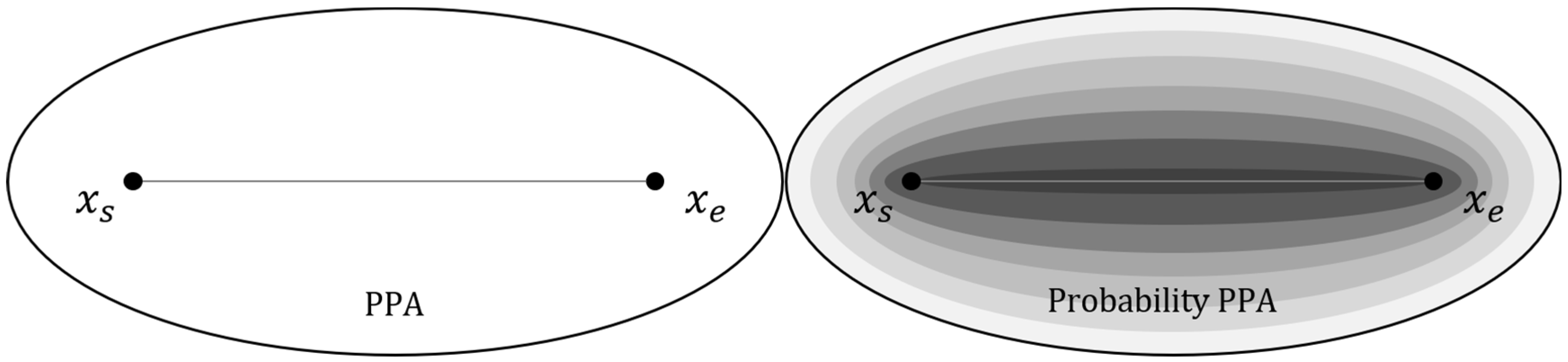
In qualitative research, time geography primarily employs three key concepts: space–time trajectories, space–time prisms, and potential path areas (PPAs) to describe space–time uncertainty [12,13,14,15]. Space–time trajectories can be viewed as time series of geographic position points, which can be represented in time geography through STP:

$$STP=\left\{l_0,l_1,\dots ,l_i,\dots ,l_n\right\}$$

(1)

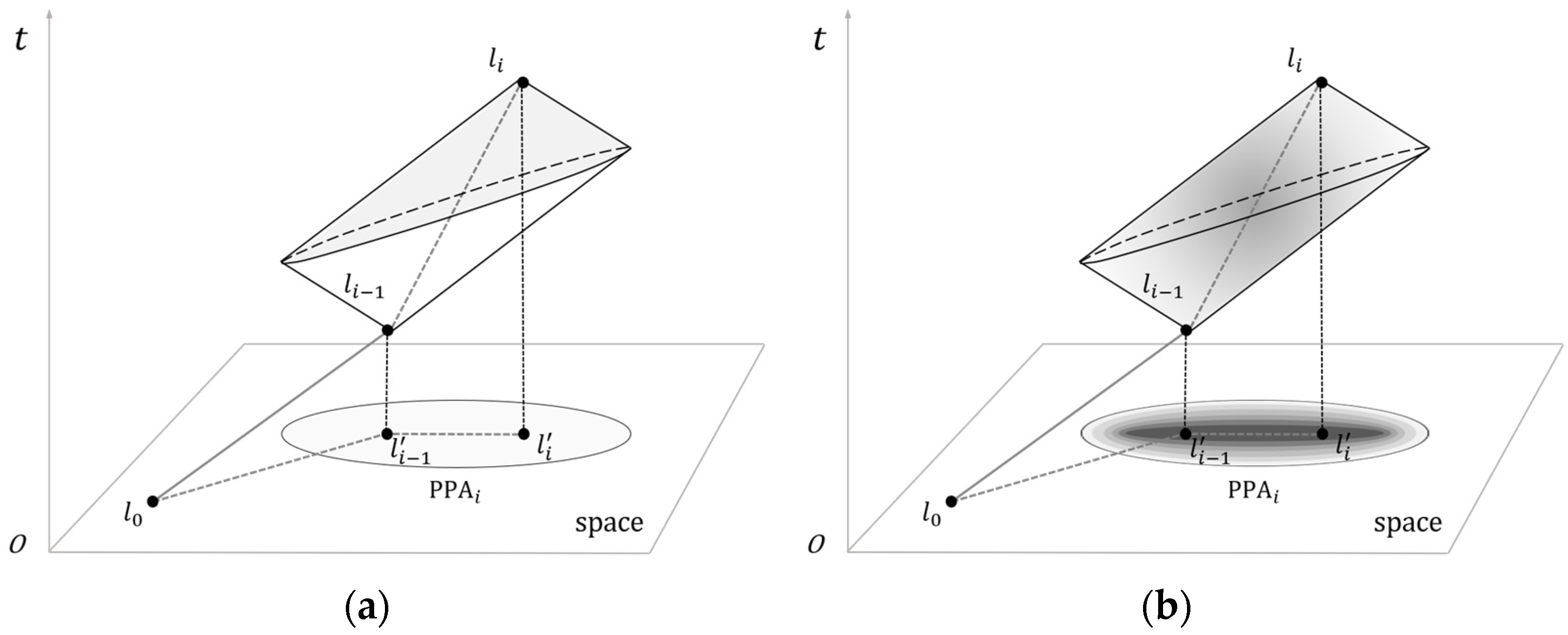
where $STP$ represents the space–time path (Figure 1); $n$ is the total number of trajectory points; and $l_i$ is the $i\mathrm{t}\mathrm{h}$ trajectory point of the moving object, which can be described as $\left(x_i,y_i,t_i\right)$, $\left(x_i,y_i\right),$ and $t_i,$ which respectively represent the two-dimensional space position and timestamp of trajectory points. Trajectory points are sometimes called anchor points or control points. The STP expresses the directional movement trend of the moving object, while the space–time prism can express the space–time boundary of the moving uncertainty. The space–time prism represents the set of all possible space–time points that a moving object can reach under the common constraints of the starting and ending points, the ability constraints (such as the maximum moving speed), and the authority constraints (such as the geographical environment) (Figure 1a). The footprint or projection of the space–time prism in the plane space is called PPA, and in the homogeneous space it can be described as an ellipse with the two anchor points ${(l}_{i-1},l_i)$ as the focal point and $v_{\mathrm{m}\mathrm{a}\mathrm{x}}·\left(t_i-t_{i-1}\right)$ as the major axis:

$${PPA}_i=\left\{x|\left|\right|x-l_{i-1}\left|\right|+\left|\right|l_i-x\left|\right|\le \left(t_i-t_{i-1}\right)·v_{\mathrm{m}\mathrm{a}\mathrm{x}}\right\}$$

(2)

where ${PPA}_i$ represents PPA on the $i\mathrm{th}$ trajectory segment, $x$ represents any point in ${\mathrm{P}\mathrm{P}\mathrm{A}}_i$, $\left|\right|-\left|\right|$ represents the Euclidean distance in two-dimensional space, $t_i-t_{i-1}$ is the budget time of each pair of trajectory anchor points $\left(l_{i-1},l_i\right)$, and $v_{\mathrm{m}\mathrm{a}\mathrm{x}}$ is the maximum moving speed of the moving object.

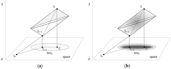
Figure 1. Basic tools of time geography: (a) space–time prism and PPA; (b) probabilistic space–time prism and probabilistic PPA.

In quantitative research, time geography assigns a position probability to each position point within a PPA or space–time prism to represent how likely it is that a moving object will access a certain reachable position at a given time. Therefore, the quantitative research of time geography is also called probabilistic time geography, which is a fusion of time geography and probability theory [8]. The basic idea is that in the PPA or space–time prism during appearance of a pair of trajectory anchor points, the position probabilities of moving objects accessing different position points at any time are not always equal, and the size of the probability value changes with the change of state information [16,17,18]. For any reachable position point, different position probabilities are typically assigned to the position points based on the time cost of reaching that point from the starting and ending points, often using distance decay kernel function models such as Brownian bridge and TGDE [7,16,19,20,21].

The qualitative and quantitative research methods of time geography analyze the space–time uncertainty of moving objects and consider the three space–time constraints of time geography. These methods are valid in homogeneous space, especially when not distinguishing the semantic attributes of position points, such as the types of POI and time semantic information. However, differences in the attachment characteristics of space position points will produce different attractions for moving objects and change over time.

2.2. POIs

A POI refers to geographic position points on a map that are of interest to moving objects, with information including position, attributes (types), and time [22,23]. People’s travel always has certain preferences and purposes [24], which is why navigation and planning are essential in people’s journeys. POIs have gradually become the key search information for people’s travel navigation [25], which is related to POIs representing certain functions and needs, and therefore has become important information for human activity analysis [26].

There are significant differences in the attractiveness of different types of POI to individuals. For example, restaurant POIs may attract people to eat, tourist attraction POIs may attract people to access, transportation facility POIs may affect people’s living habits and travel choices, shopping consumption POIs may affect people’s consumption behaviors, and so on. The space distribution of POI positions usually has a certain aggregation [27]. For example, a large number of various service types of POIs are gathered in urban business districts, so as to attract nearby consumers to travel.

The same types of POIs will have different attraction to individuals at different time periods [28,29,30]. For example, the attraction of restaurant POIs to individuals at mealtime is much higher than that at other time; the attraction of corporate POIs to individuals is greater on working days; and the attraction of tourist attraction POIs is generally greater on holidays. POIs can better reflect the space–time activity behavior of urban residents and have a strong explanatory power for the behavior of moving objects accessing the space–time position points. Therefore, it is necessary to consider the actual POI semantic information in the quantitative calculation of position probability.

2.3. POIs in Time Geography

Based on the analysis above, it can be concluded that the attractiveness of POIs has an impact on the access of moving objects. The quantitative description of this influence will affect the calculation of position probability. The activity of an individual moving object usually includes various POI position points, and there is space–time proximity between the space–time trajectories of moving objects and the accessed POI positions. Existing studies have analyzed the attractiveness of POIs from two aspects.

Zeng proposed a method to analyze the change of attraction of urban POIs based on a taxi track [31]. He calculated the attractiveness and distribution of different categories of POI in different time periods according to the proximity of taxis staying near different categories of POIs in different time periods and then statistically analyzed the law of citizen activities. He believes that the attractiveness of POIs is related to their attributes, position, and time period, and that existing methods ignore the influence of time and category on the attractiveness of POIs. This method evaluates the attractiveness of POIs through statistical analysis and presents the distribution of POIs in a large range of global attractiveness but ignores the semantic information of POIs themselves and the personalized attractiveness of POIs to a single space–time trajectory. Moreover, this method requires a large number of independent trajectory data samples and lacks a priori in calculating the probability distribution. Downs assigns access probabilities to space positions including POI positions using TGDE [2], and the access probability of POI positions reflects the attraction of the POIs to moving objects. This method only considers the start and end points of space–time trajectories, without considering the time budget of corresponding activities at POI positions. This method also ignores the semantic information of POIs, and it lacks verification of the posterior probabilities of POI access based on empirical data.

The above research indicates that the influence of POI semantic information on the trajectory of moving objects is significantly different, and correspondingly, the possibility of moving objects on the same trajectory accessing POIs with different attractiveness is also different. In time geography, on the one hand, the attraction of POIs is an uncertainty measure of space–time position points, which is the probability of space–time position statistics through a large number of space–time trajectories. On the other hand, relative to the space–time trajectory, POIs are the position points that the moving object can reach in space–time, and the access activity at the POI position points is also a part of the time budget between the anchor points of the space–time trajectory.

Therefore, the time geography based on space–time trajectory to predict space–time uncertainty needs to incorporate the semantic information of POIs into the position probability distribution, including POI type, time factor, etc. At present, TGDE only considers the space position and the time cost from the position point to the two anchor points, without considering the difference of POIs in space positions. In this paper, a POI probability model considering the proximity of moving trajectories is proposed based on the known trajectory information and the space–time distance between the trajectory point and the POI. The model expresses the space–time uncertainty between known precise space–time position points based on the space–time constraints of moving speed and time limitations and provides all the information, including time, space, and semantic information, for this space–time uncertainty measurement, which avoids the error caused by single information. This model not only provides a theoretical basis for the quantification of position probability but also provides a time geography support for the statistics of POI attraction. For example, in the space–time prism of a moving object, the trajectory that does not contain a POI can be excluded when calculating the space–time trajectory of a moving object passing through a POI.

3. Construction of the POI Access Probability Model

There is an interaction between the activity of the moving object and the POI position point: the activity and the flow of people it brings will affect the space layout of the POI. Conversely, the aggregation of the POI will also attract the accessing of the moving object. This means that the POI access probability considers not only the activity trajectory but also the characteristics of the POI itself, such as position, type, and opening time. Therefore, the access probability of POIs is not only related to their own space position, but also to their non-position information, involving the semantic information such as the attribute and time of the POI. The quantitative analysis of POI position assignment probability via time geography requires that POI position information and non-position information be treated as equally important.

3.1. POI Position Probability

In space, there are many factors that affect the access probability of POI position points, such as weather, distance, travel route direction, and POI characteristics themselves. In this paper, the time geography kernel density estimation function TGDE is used to calculate the position probability of a POI position point being accessed based on the space–time distance cost, and the normalized access probability can be formalized as follows:

$$P_{\mathrm{s}\mathrm{p}\mathrm{a}\mathrm{c}\mathrm{e}}^{\prime }({POI}_k)=\frac{P_{\mathrm{s}\mathrm{p}\mathrm{a}\mathrm{c}\mathrm{e}}({POI}_k)}{\sum P_{\mathrm{s}\mathrm{p}\mathrm{a}\mathrm{c}\mathrm{e}}({POI}_k)}$$

(3)

where ${POI}_k$ is the $k\mathrm{t}\mathrm{h}$ POI position point in the PPA, $P_{\mathrm{s}\mathrm{p}\mathrm{a}\mathrm{c}\mathrm{e}}\left({POI}_k\right)$ is the position probability of the $k\mathrm{t}\mathrm{h}$ POI position point in the PPA, and $P_{\mathrm{s}\mathrm{p}\mathrm{a}\mathrm{c}\mathrm{e}}^{\prime }\left({POI}_k\right)$ is the position probability after normalization.

3.1.1. Sample Space PPA

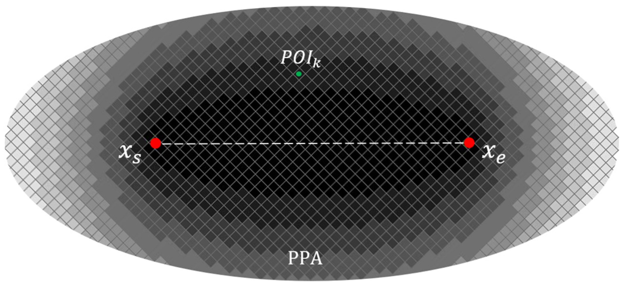
A key concept in time geography is PPA, which represents the reachable range of a moving object under the constraints of two space–time trajectory points. PPA provides a sample space for the measure of POI access probability, which can be mathematically described as an ellipse with a pair of starting and ending anchor points ${(x}_s,x_e)$ as the focus and $v_{\mathrm{m}\mathrm{a}\mathrm{x}}·t\left(s,e\right)$ as the long axis in homogeneous space (Figure 2). The PPA during a pair of anchor points can be formalized as follows:

$$PPA=\left\{x|\left|\right|x-x_s\left|\right|+\left|\right|x-x_e\left|\right|\le t\left(s,e\right)·v_{\mathrm{m}\mathrm{a}\mathrm{x}}\right\}$$

(4)

where $t\left(s,e\right)$ represents the time budget from anchor point $s$ to anchor point $e$, which is the difference in time at the two anchor points.

Figure 2. PPA and probability PPA.

From the above, it is clear that PPA is an ideal model with only two variables: trajectory time budget and maximum possible speed. In reality, especially when describing human activities, the maximum possible speed varies greatly between different modes of travel, such as walking (5 km/h) and driving (50 km/h, a smaller estimate in cities). Despite the widespread use of PPA, its main limitation is that when the maximum speed or time budget is large enough, the PPA is too large or even beyond the study area, thus making it lose the physical significance of delimiting the reachable area.

A common approach is to use the probability density function to narrow down the PPA, which is the probability PPA (Figure 2). For example, in motion ecology, 50% and 95% TGDE isodensity lines are used instead of PPA boundaries as the core home range and home range [3], based on the theory that the access probability within the space–time prism is not uniform [16]. The premise of the above method is to assign a probability to each position point within the PPA to measure the likelihood of the moving object being in that position at a particular time [18]. The use of isodensity lines instead of PPA boundaries can greatly reduce the scope of the study, thus helping to improve the expression of PPA. At the same time, this reduction can also allocate limited resources such as fire protection, policing, and commerce to areas that are accessed more frequently by people, thereby improving the utilization rate of social resources and the energy efficiency of services.

3.1.2. Position Probability of Sample POI

Generally, there are two methods used to calculate the probability of position points in the plane space. One method is to cover the entire research area with a regular grid, then calculate the probability values of all positions in the research area one by one, and finally select the probability value containing the required POI position points. The other method is to calculate the probability value at a single point element by considering only the POI points where the position probability needs to be calculated. The former requires a large amount of computation, while the latter is a discrete POI probability that cannot generate a continuous probability surface [32,33].

In this paper, we use the first method. We calculate probabilities using a regular grid covering the PPA range to generate a continuous probability surface that represents the probability of POI accessing positions. According to the sum of the distance between any position $x$ in the PPA and the two anchor points $(x_s,x_e)$, i.e., $\left|\right|x-x_s\left|\right|+\left|\right|x_e-x\left|\right|$, the probability is assigned to each position point in a PPA by combining TGDE and the space connection method (Figure 3). It can be formalized as follows:

$$P_{\mathrm{s}\mathrm{p}\mathrm{a}\mathrm{c}\mathrm{e}}\left(x\right)=G(\frac{\left|\right|x-x_s\left|\right|+\left|\right|x_e-x\left|\right|}{t\left(s,e\right)·v_{max}})=\frac{t\left(s,e\right)·v_{max}}{\left|\right|x-x_s\left|\right|+\left|\right|x_e-x\left|\right|}$$

(5)

where $G(·)$ is an attenuation function. $t\left(s,e\right)·v_{max}$ is the maximum activity distance of a moving object during a pair of locus anchor points, which is used to replace the bandwidth of the classical kernel density function [3]. TGDE realizes the fusion of kernel density estimation and time geography, which avoids the deviation of density estimation caused by the classical kernel density estimation assigning non-zero probability to the position outside the geographic ellipse and also avoids the deviation caused by the subjective setting of the bandwidth.

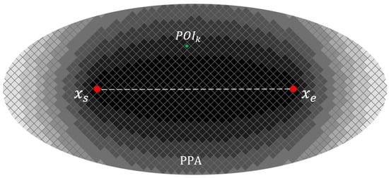
Figure 3. TGDE.

3.2. POI Time Weight

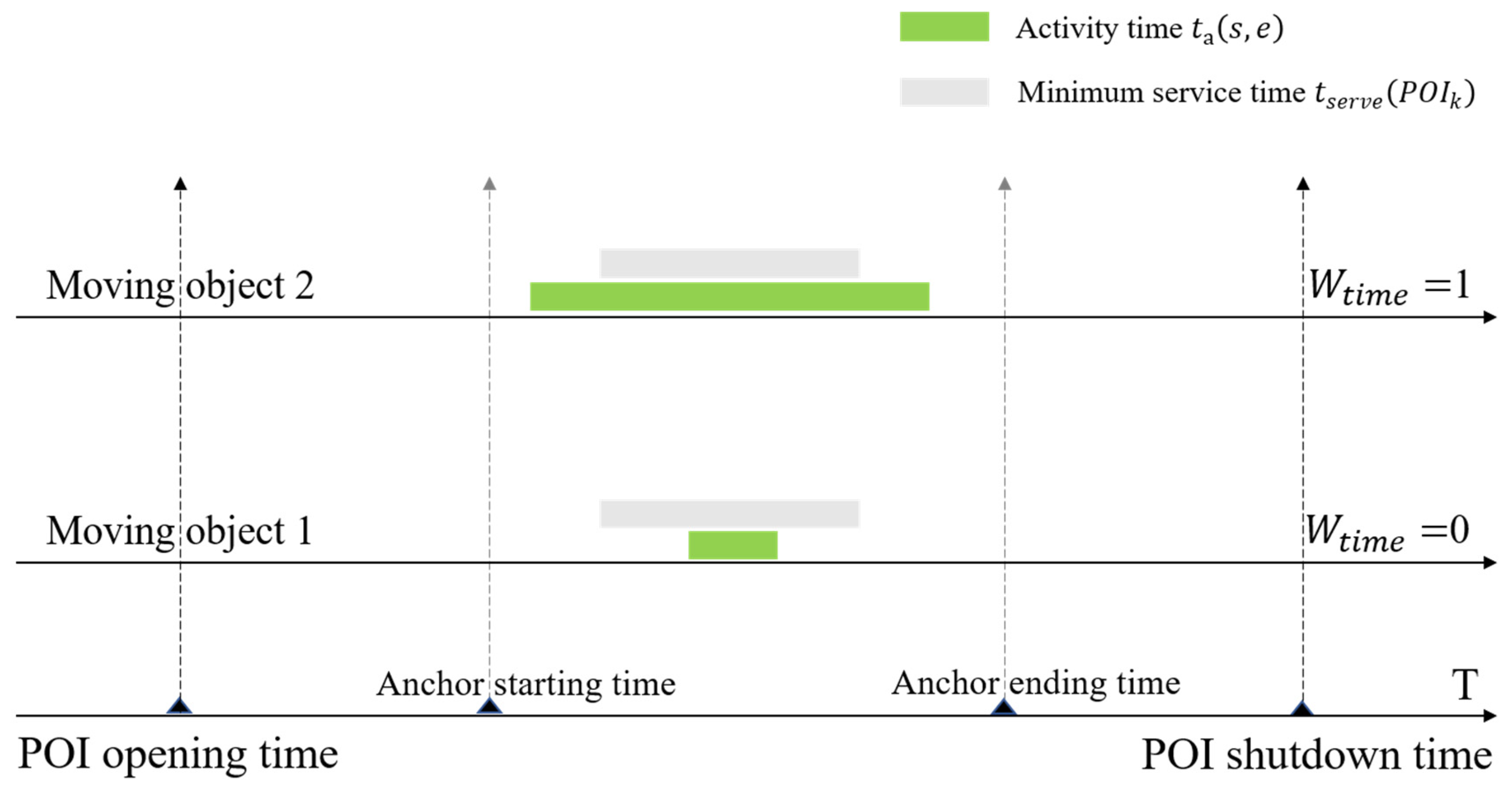
In terms of time factors, POI time weights can be divided into two aspects: the time of the moving objects and the time of the POI. Among them, the time of the moving object includes the time period between adjacent trajectory points and the activity time. The time of the POI includes two time periods: open time and minimum service time (Figure 4). If the active time includes the minimum service time of the POI, and the active time is within the open time of the POI, the time weight factor of the POI is 1, otherwise it is 0. The time weight of a POI can be formalized as follows:

$$W_{time}({POI}_k)=\left\{\begin{array}{l}1, {t_{serve}\left({POI}_k\right){\subseteq t}_a\left(s,e\right) \& t_a\left(s,e\right)\subseteq t}_{open}\left({POI}_k\right)\\ 0, \mathrm{otherwise}\end{array}\right.$$

(6)

where $W_{time}\left({POI}_k\right)$ represents the time weight of the $k\mathrm{t}\mathrm{h}$ POI position point, $t_{serve}\left({POI}_k\right)$ represents the minimum service time of the POI, $t_{\mathrm{a}}\left(s,e\right)$ represents the activity time of the moving object during a pair of trajectory anchor points, and $t_{open}\left({POI}_k\right)$ represents the open time of the POI.

Figure 4. Time weight of POI.

3.2.1. The Time of the Moving Objects

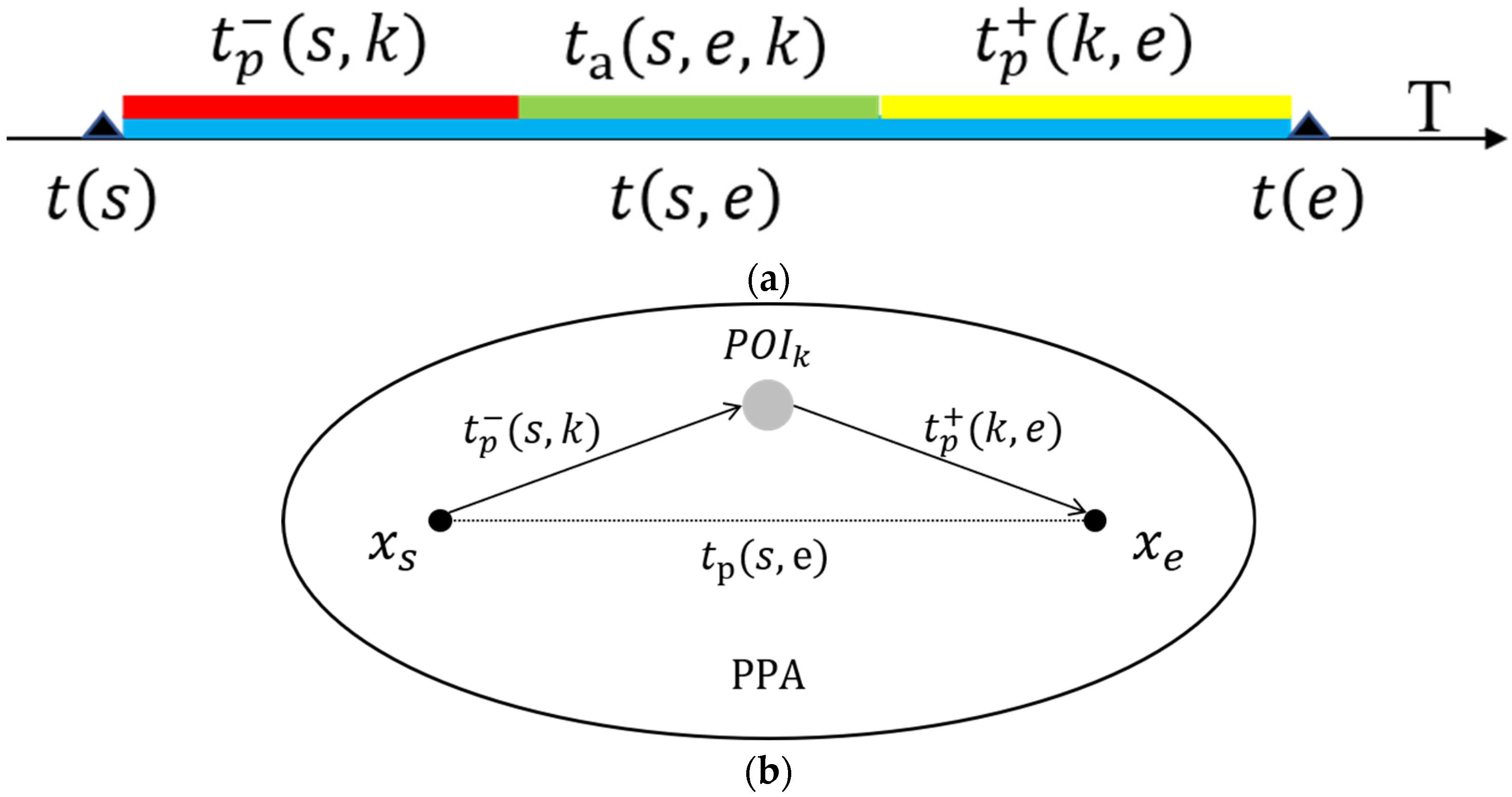
The time of moving objects includes two aspects: the time period between adjacent trajectory points and the activity time (Figure 4). The time period between adjacent trajectory points refers to the budget time $t\left(s,e\right)$ between each pair of space–time trajectory anchors. Activity time refers to the time period except the minimum moving time of route ${POI}_k$ within the budget time between each pair of space–time trajectory anchors $\left(s,e\right)$, which is expressed as $t_{\mathrm{a}}\left(s,e,k\right)$; the active time is a subset of the time period between adjacent trajectory points. Thus, $\mathrm{b}\mathrm{u}\mathrm{d}\mathrm{g}\mathrm{e}\mathrm{t} \mathrm{t}\mathrm{i}\mathrm{m}\mathrm{e}=[\mathrm{l}\mathrm{e}\mathrm{f}\mathrm{t} \mathrm{m}\mathrm{o}\mathrm{v}\mathrm{e} \mathrm{t}\mathrm{i}\mathrm{m}\mathrm{e}+\mathrm{a}\mathrm{c}\mathrm{t}\mathrm{i}\mathrm{v}\mathrm{e} \mathrm{t}\mathrm{i}\mathrm{m}\mathrm{e}+\mathrm{r}\mathrm{i}\mathrm{g}\mathrm{h}\mathrm{t} \mathrm{m}\mathrm{o}\mathrm{v}\mathrm{e} \mathrm{t}\mathrm{i}\mathrm{m}\mathrm{e}]$ (Figure 5a). The time to move left is the minimum time cost from $s$ to ${POI}_k$, $t_p^{-}(s,k)$; right shift time is the minimum time cost from ${POI}_k$ to $e$, $t_p^{+}(k,e)$. It is worth mentioning that the sum of the left and right movement times is different from $t_{\mathrm{p}}(s,e)$, which is the minimum time cost from $s$ to $e$ [34].

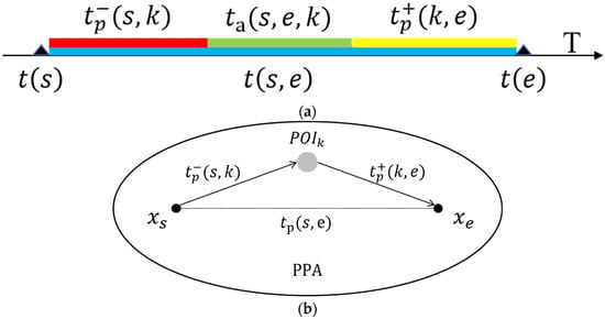
Figure 5. Time of moving objects: (a) activity time diagram; (b) POI diagram of moving object path.

There is uncertainty in the space–time information of the mobile object during the budget time, and it is impossible to accurately obtain the space–time trajectory of the moving object in this time period. However, the activities of the moving object usually occur at POI position points, especially in urban space. This means that the ascertained POI distribution can provide a theoretical basis for quantifying the space–time uncertainty of moving objects.

When people carry out various social activities, they always try to obtain the greatest benefit at the least cost, so we can reasonably assume that the moving object moves the least time before and after the activity destination. The minimum time spent on the road by a moving object passing through a POI position at maximum walking speed within the PPA can be formalized as follows:

$$t_{\mathrm{p}}\left(s,e,k\right)=t_p^{-}\left(s,k\right)+t_p^{+}(k,e)=\frac{\left|\right|{POI}_k-x_s\left|\right|+\left|\right|{x_e-POI}_k\left|\right|}{v_{\mathrm{m}\mathrm{a}\mathrm{x}}}$$

(7)

where $t_{\mathrm{p}}(s,e,k)$ represents the minimum time spent on the road by the moving object. $\left|\right|{POI}_k-x_s\left|\right|$ and $\left|\right|{x_e-POI}_k\left|\right|$ are the two-dimensional distances from the anchor point to the POI position point (Figure 5b). Thus, the activity time can be formalized as follows:

$$t_{\mathrm{a}}\left(s,e,k\right)=t\left(s,e\right)-t_{\mathrm{p}}(s,e,k)$$

(8)

3.2.2. The Time of POI

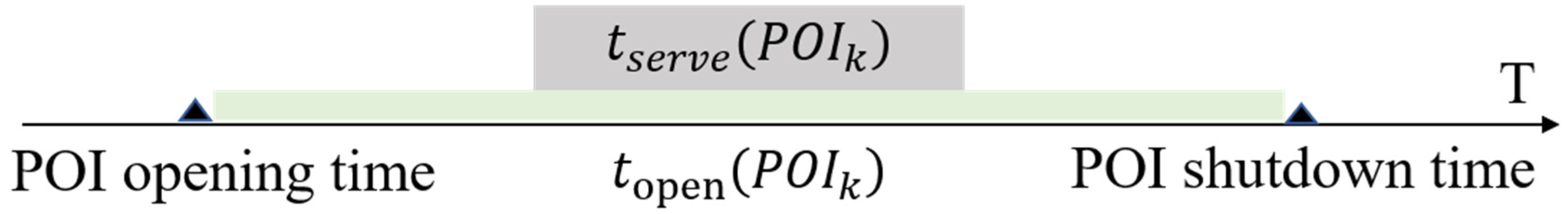
The time of a POI includes two time periods: open time and minimum service time (Figure 6). Open time refers to the business hours of POI points, such as the opening hours of barber shops being mostly 09:00~22:00. Minimum service time refers to the minimum time required for a moving object to perform the corresponding activities at a POI position point when it accesses the POI position point, such as the minimum time required for a haircut at a barber shop being 10 min. In addition, the minimum service time should include the queue wait time, and here the queuing time is regarded as 0. For example, Table 1 gives the minimum service time for five types of POI (ATM, restaurant, shopping, science and education (SE), and sports). The minimum service time period is a subset of the open time period and determines the types of activities that a moving object can perform during the active time.

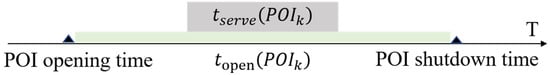
Figure 6. Time of POI.

Table 1. Minimum service time of POI.

POI Type	ATM	Restaurant	Shopping	SE	Sports
Minimum service time (min)	5	20	20	5	20

In real space, POIs have diversity, and the time characteristics of different types of POI have great differences, mainly in the open time period and the minimum service time period. For example, most of the open times of elementary schools are 09:00~17:00, which is different from the open time of barber shops. Therefore, the time factor cannot affect the access weight of the POI alone but needs to be combined with the type of POI.

3.3. POI Type Weight

At different points in time, moving objects have different access preferences for different types of POI, so different types of POI position points have different semantic weights at different points in time; for example, people go out to their businesses in the morning and return to their homes in the evening. This means that the POI type, as a single attribute, needs to be combined with the time attribute to better describe changes in the attractiveness of the POI to moving objects.

3.3.1. POI Type

The types of different POIs play a decisive role in people’s access. According to Google Maps, the types of POI include restaurant, company, shopping, transportation facility, hotel, tourist attraction, SE, finance and insurance, residence, etc. [35]. Different types of POIs can meet people’s different needs.

People’s needs change over time. This means that people access different types of POIs at different times; in other words, the same POI appeals to people differently at different times. Therefore, the same POI has different preferences to be accessed at different points in time, and correspondingly, the preferences to access different types of POIs at the same point in time are different.

According to life experience and data observation, a day is divided into six periods: [06:00, 09:00], [9:00, 12:00], [12:00, 14:00], [14:00, 18:00], [18:00, 22:00], and [22:00, 06:00⁺¹] [31]. Table 2 shows the type weights of the five types of POI (ATM, restaurant, shopping, SE, sports) visited, but this is only an example, which can be dynamically adjusted according to the living habits of local people in different urban scenarios. For example, between [12:00, 14:00], moving objects are more likely to access the POI of restaurant, while between [14:00, 18:00], moving objects are more likely to access the POI of shopping.

Table 2. Type weights of POI.

Time	ATM	Restaurant	Shopping	SE	Sports
[06:00, 09:00]	0.15	0.4	0.15	0.15	0.15
[09:00, 12:00]	0.2	0.3	0.3	0.1	0.1
[12:00, 14:00]	0.15	0.4	0.2	0.15	0.1
[14:00, 18:00]	0.2	0.2	0.3	0.2	0.1
[18:00, 22:00]	0.2	0.3	0.2	0.1	0.2
[22:00, 06:00+1]	0.2	0.2	0.2	0.2	0.2

From the above table, it can be seen that people’s activity needs establish a bridge between POI types and activity trajectory point timestamps, and the attractiveness of different types of POI varies non-uniformly over time. This provides a quantitative basis for calculating the preference of moving objects to access any POI type based on the timestamps of trajectory points.

3.3.2. Calculating the POI-Type Weight

In time geography, a PPA of a moving object has two time points corresponding to two space–time anchors. For either of the two time points, we can assign a weight to any POI within the PPA according to Table 2. At present, there is not enough information and no perfect theory to support the weight allocation of the same POI at two time points. For a PPA, a POI should have a type weight, and POIs of the same type should have the same type weight. This means that the POI-type weights corresponding to the two timestamps of the two anchor points within the PPA need to be fused. However, this can cause certain errors, such as the weight possibly being very low at the start and end times and very high between them; then, the type weight assigned to the POI will be less than it should be. Based on this, when we calculate the POI-type weight, we fuse the type weight of the start anchor timestamp, the type weight of the anchor middle timestamp, and the type weight of the end anchor timestamp. They are fused by calculating the average:

$$W_{class}({POI}_k)=\frac{W_{class}^s\left({POI}_k\right)+W_{class}^e\left({POI}_k\right)+W_{\raisebox{1ex}{$t$}\!\left/ \!\raisebox{-1ex}{$2$}\right.}\left({POI}_k\right)}{3}$$

(9)

where $W_{class}\left({POI}_k\right)$ represents the type weight of the $k\mathrm{t}\mathrm{h}$ POI position point, $W_{class}^s\left({POI}_k\right)$ represents the POI-type weight determined by the start anchor timestamp, $W_{\raisebox{1ex}{$t$}\!\left/ \!\raisebox{-1ex}{$2$}\right.}\left({POI}_k\right)$ represents the POI-type weight determined by the anchor middle timestamp, and $W_{class}^e\left({POI}_k\right)$ represents the POI-type weight determined by the end anchor timestamp. The normalized type weights can be formalized as follows:

$$W_{class}^{\prime }({POI}_k)=\frac{W_C\left({POI}_k\right)}{\sum W_C\left({POI}_k\right)}$$

(10)

where $W_{class}^{\prime }\left({POI}_k\right)$ represents the normalized POI-type weights.

3.4. POI Access Probability Model

In this paper, the distribution of position probability is extended from feedback to mutual feedback. The traditional calculation method of position probability is the calculation of the time cost from the space–time anchor point to the point to be measured, and it only considers the ability constraint, that is, the moving speed and time of the moving object, which is one-way feedback. However, in urban space, the position of people’s activities usually contains various types of POI, and there are often preferences about time and space position when selecting activities. This preference can also be interpreted as the influence of POI semantic information of the point to be measured on the access of the moving object. For example, the moving object will not access the supermarket that is closed after 22:00; that is, the access probability is 0, which belongs to the authority constraint.

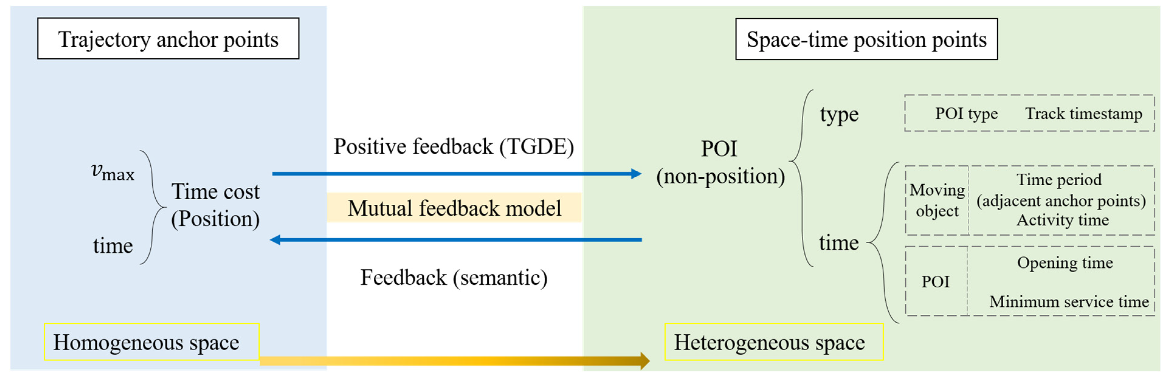
Therefore, in this paper, we will start with the time and space factors of the space–time trajectory, and we will add the non-position weight (time and type) to the POIs on the basis of adding the position probability. In space, the probability of space position is assigned based on TGDE. In terms of time, semantic weights are assigned based on POI time and type. A mutual feedback mechanism between anchor points and POI position points is formed (Figure 7), which integrates space–time semantic information to measure the probability of moving objects accessing POI points of various types of uncertainty between deterministic space–time trajectory points. In this way, in urban heterogeneous space, we will have a probabilistic time geographic modeling method considering POI semantics.

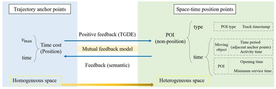
Figure 7. Mutual feedback model.

Combining position probability and non-position weight, the product of the two can be used to calculate the access probability of POI position points. The probability calculation equation of the “Mutual feedback model” is as follows:

$$({POI}_k)=\frac{P_{space}^{\prime }\left({POI}_k\right)W_{time}\left({POI}_k\right)W_{class}^{\prime }\left({POI}_k\right)}{\sum P_{space}^{\prime }\left({POI}_k\right)W_{time}\left({POI}_k\right)W_{class}^{\prime }\left({POI}_k\right)}$$

(11)

where $P\left({POI}_k\right)$ represents the access probability of the $k\mathrm{t}\mathrm{h}$ POI position point.

4. Experimental Setup

4.1. Data Source

The experimental data required in this paper are trajectory data containing specific activity information of individual moving objects. The data mainly come from trajectory data uploaded by users of the 2bulu website (https://www.2bulu.com, accessed on 30 July 2023), which includes information such as the time series of departure points, destinations, and activity labels. These trajectories are located in Shenzhen, Guangdong Province, China, in terms of spatial position. Spatial data sources are obtained from the open-source map, OpenStreetMap (https://www.openstreetmap.org, accessed on 6 May 2023). Additionally, 392,500 pieces of POI data for this area were obtained through Python web scraping, including attributes such as names, types, and geographic coordinates. POIs are discrete point features on the map, and to continuously depict the access probability of moving objects in the plane space, the method proposed in this paper will be applied to a spatial regular grid C (10 m × 10 m). The implementation of this model is based on ArcGIS 10.2 (ESRI, Inc., Redlands, CA, USA).

4.2. Calculation of POI Access Probability

(1)

Method

Based on the principles of space–time paths in time geography, as expressed in Equation (1), the space–time trajectories of moving objects are obtained and formalized to generate sequences of space–time anchor points, constructing the STPs of individual moving objects. Each STP is composed of time-adjacent trajectory anchor points and line segments connecting them. The anchor point data include space positions (longitude, latitude) and time labels (DD Month YYYY hh:mm:ss). The STP constructed in this paper contains 8 trajectory anchor points, with a time interval from 10 September 2022 6:10:00 to 10 September 2022 9:30:00, STP = {(1, 114°6′31.800″ E, 22°32′40.693″ N, 10 September 2022 6:10:00), (2, 114°6′23.872″ E, 22°32′40.427″ N, 10 September 2022 6:30:00), (3, 114°6′25.452″ E, 22°32′29.717″ N, 10 September 2022 7:20:00), (4, 114°6′54.252″ E, 22°32′34.397″ N, 10 September 2022 8:50:00), (5, 114°6′51.098″ E, 22°32′39.786″ N, 10 September 2022 9:00:00), (6, 114°6′48.298″ E, 22°32′39.098″ N, 10 September 2022 9:10:00), (7, 114°6′47.635″ E, 22°32′45.802″ N, 10 September 2022 9:20:00), (8, 114°6′38.855″ E, 22°32′45.157″ N, 10 September 2022 9:30:00)}. The vertical dimension of the three-dimensional space–time path represents time height. There is a relative difference between the space and time dimensions of the STP, so the height of the time dimension is somewhat subjective relative to the space position, considering the effect of three-dimensional display.

In this paper, we set $v_{max}=1 \mathrm{m}/\mathrm{s}$. Based on the STP constructed in the previous step and the principles of space–time prisms in time geography, as expressed in Equation (2), a PPA of a moving object is constructed between a pair of anchor points ((3, 114°6′25.452″ E, 22°32′29.717″ N, 10 September 2022 7:20:00), (4, 114°6′54.252″ E, 22°32′34.397″ N, 10 September 2022 8:50:00)), and a space regular grid C (10 m × 10 m) covering the PPA is generated. This paper takes the types of POI that represent the behavioral activities of moving objects as examples and selects five types of POI: ATM, restaurant, shopping, SE and sports. Restaurant POIs include Chinese restaurant, fast food restaurant, tea restaurant, and comprehensive restaurant. Shopping POIs include supermarkets and shopping malls; SE POIs include schools and training institutions; and sports POIs include park squares, sports venues, and fitness centers. By using PPA and POI point sets within the study area for intersection calculation, 3526 POI points were selected to prepare for the next step of assigning position probability and non-position weight to the POI.

Moving objects will have travel cost considerations when choosing a destination to access. The POI that spends less time on the road and is closer together is usually given priority. Based on the preference of space–time distance cost, the position probability of each cell in the grid space is calculated according to Equation (3). The space connection method is used to match the grid cells and POI position points one by one. When multiple POIs fall into the same grid cell, the position probability is regarded as the same. In this way, we will calculate the position probability of each POI position within the PPA being accessed. In order to continuously describe the position probability of moving objects on the plane space, a continuous POI position probability surface is generated using Inverse Distance Weighting (IDW) interpolation.

The attractiveness of POIs represents people’s “expectation” and “preference” for a certain type of POI, and its non-position weight can describe the characteristics of POIs themselves well. The time factor and type of POI affect the preference of moving objects to access POI position points. During a pair of anchor points (s [10 September 2022 7:20:00], e [10 September 2022 8:50:00]), 1174 sports, SE, and ATM POIs are all within the opening time, among which 1055 POIs have an activity time greater than the minimum service time; according to Equation (6), their time probability is 1, while the time probability for the remaining POIs is 0. Among the 2352 restaurant and shopping POIs, there are 1571 POIs in the opening time, and the activity time is greater than the minimum service time, with the time probability of 1 and the remaining POI time probability of 0. From the type weight of a POI (Table 2), it can be seen that the time interval of the anchor point is within the same time interval; therefore, based on Equation (10), the type weights of ATM, restaurant, shopping, SE, and sports POIs are 0.15, 0.4, 0.15, 0.15, 0.15, and 0.15, respectively.

Finally, fusing position probability and non-position weight, according to Equation (11), the probability of a POI position point being accessed considering the POI semantics is computed. In order to continuously describe the access probability of moving objects on the plane space, a continuous POI access probability surface is generated via IDW interpolation.

(2)

Results

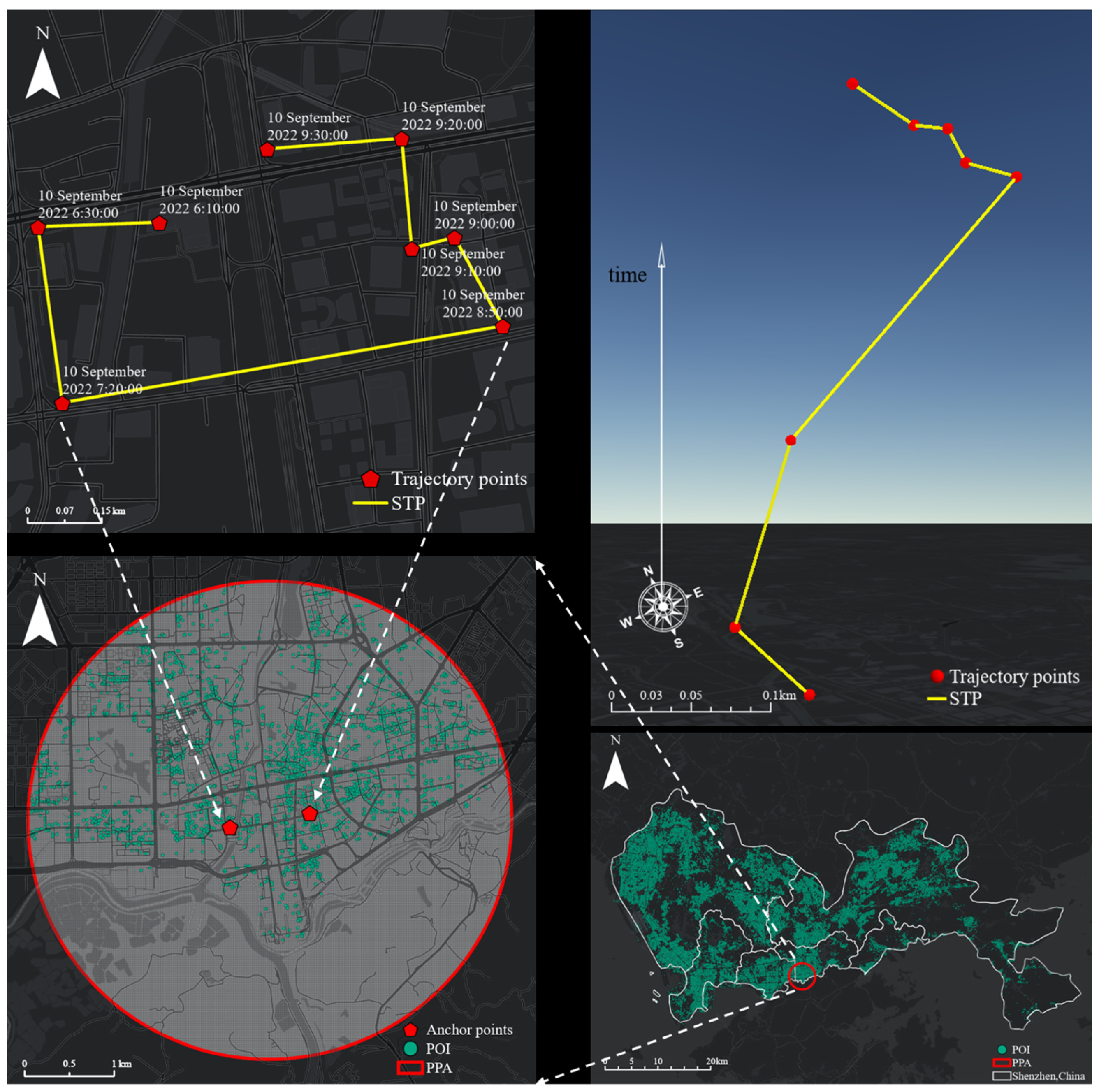
Figure 8 illustrates 2D (top left) and 3D (top right) forms of a space–time path, POI (bottom right), and a PPA (bottom left) in the study area. In Figure 8, the red points represent trajectory anchor points, yellow lines represent the space–time paths, green points represent POIs, and red circles represent PPAs. In a 2D map, time information is ignored when the moving trajectory is expressed by point and line elements, while in a 3D map, the space–time trend of moving objects is depicted by adding vertical time semantic information, which enhances the visualization effect. PPA is an ideal model with only two variables: track time budget and maximum possible moving speed. In Figure 8, the time interval of the two anchor points is 90 min, and the time budget is large enough, so the PPA ellipse approximates a circular shape. In this PPA, ATM, restaurant, shopping, SE, and sports POIs accounted for 7%, 60%, 6%, 18%, and 9%, respectively. It can be seen that the urban function of this area is mainly to satisfy the needs of people for food and education.

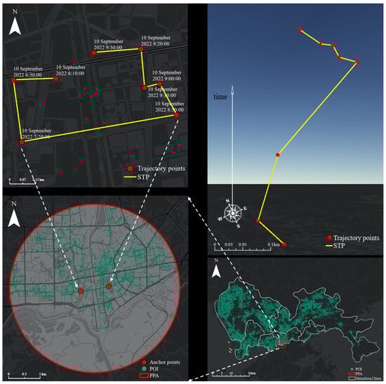
Figure 8. Study area, a trajectory, and a PPA.

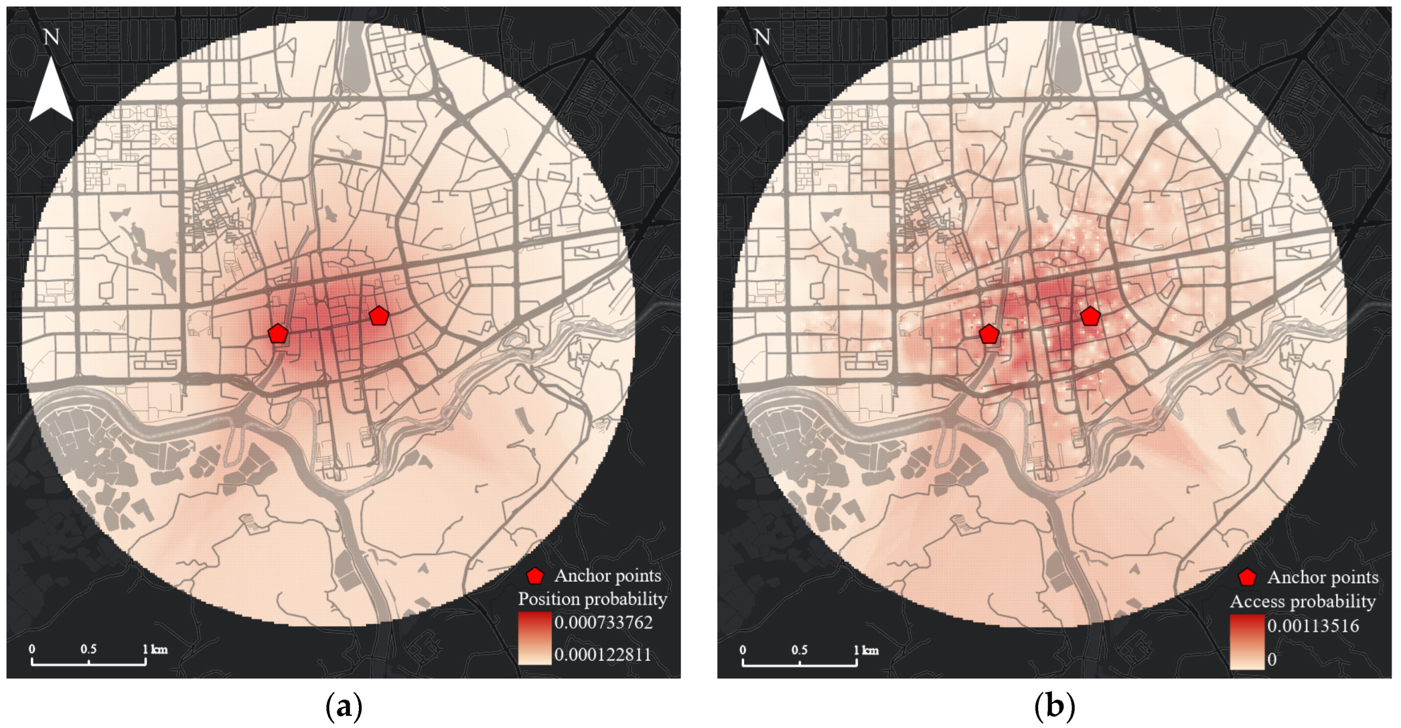
Figure 9 illustrates the POI position probability surface and access probability surface. The darker the color, the greater the probability value. In Figure 9a, the continuous POI position probability surface is generated via IDW interpolation from the POI position probability calculated using TGDE. These surfaces do not consider non-position attributes of a POI. The POI position probability value is larger on the line of anchor points and near the anchor points, and the POI position probability decreases uniformly with the increase of distance from the anchor points. At the edge of the PPA, the POI position probability is infinitely close to 0. In Figure 9a, the continuous POI access probability surface is generated using IDW interpolation from the POI access probability calculated using the “Mutual feedback model” proposed in this paper. These surfaces consider non-position attributes (type and time) of POIs. Compared with Figure 9a, POI access probability decreases non-uniformly as the distance from anchor points increases. In this paper, on the basis of position probability, it is more realistic to assign 0 probability to POIs where the moving object appears at POI non-opening times, or the activity time is less than the minimum service time. In contrast, TGDE assigns a non-0 probability to every POI, which does not correspond to reality.

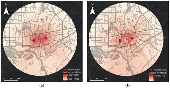
Figure 9. POI probability surface: (a) position probability surface; (b) access probability surface.

4.3. Verification

In order to test the validity of the proposed model, this paper counts the real distribution of the access probability of POI position points through individual trajectory data originated from data sources. Subsequently, the Root Mean Square Error (RMSE) was employed to evaluate the average deviation between the theoretical distribution generated using the model in this paper and the real distribution: [36]

$$RMSE=\sqrt{\frac{1}{n}{\sum }_1^n{(O_k-P_k)}^2}$$

where $O_k$ and $P_k$ represent the real and theoretical values at ${POI}_k,$ respectively, and $n$ represents the number of samples. A lower $RMSE$ value indicates higher model accuracy. In addition, we also calculate the RMSE of the theoretical distribution generated using TGDE and the real distribution to demonstrate the superiority of the “Mutual feedback model” proposed in this paper compared to the classical TGDE model.

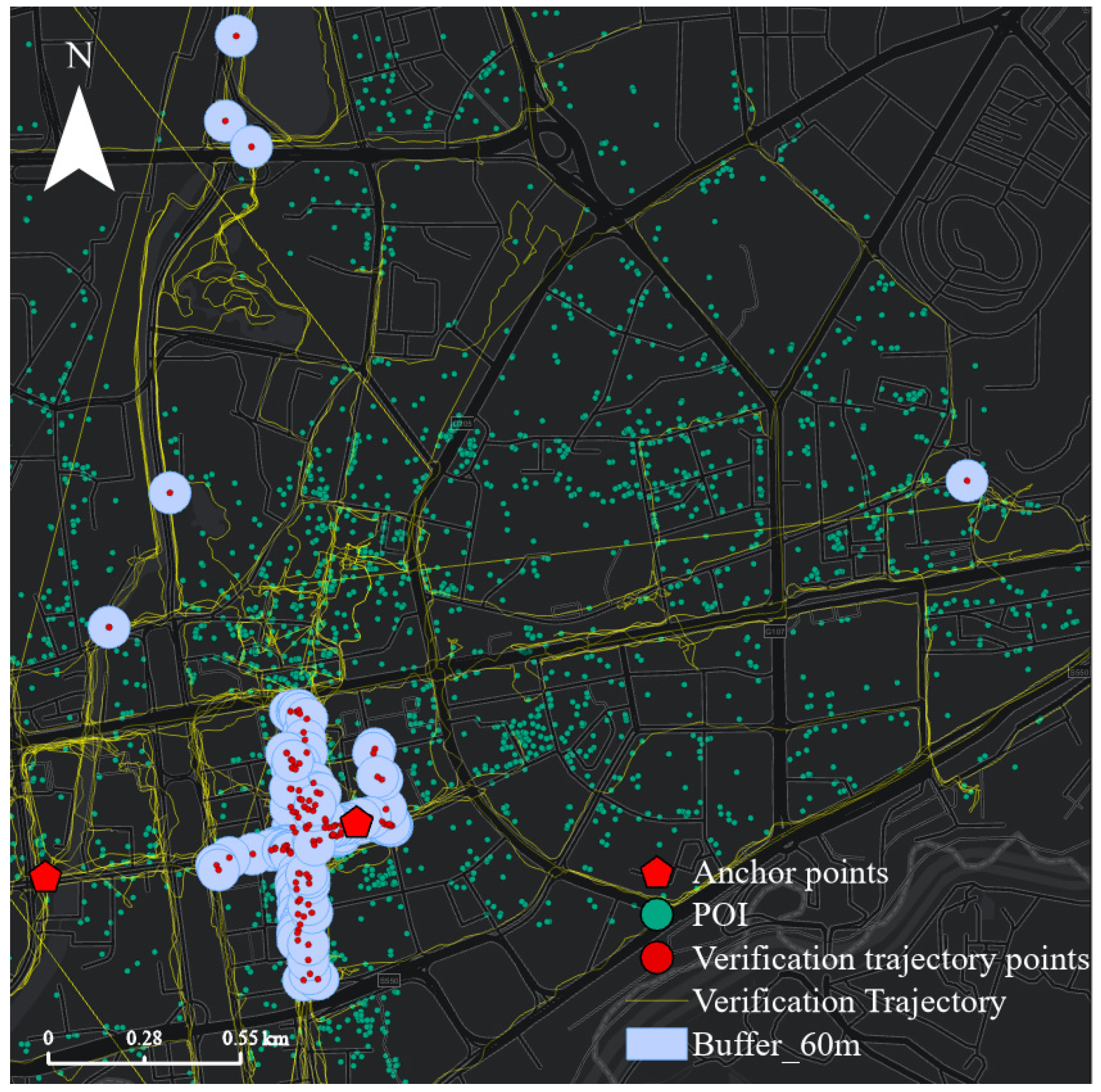
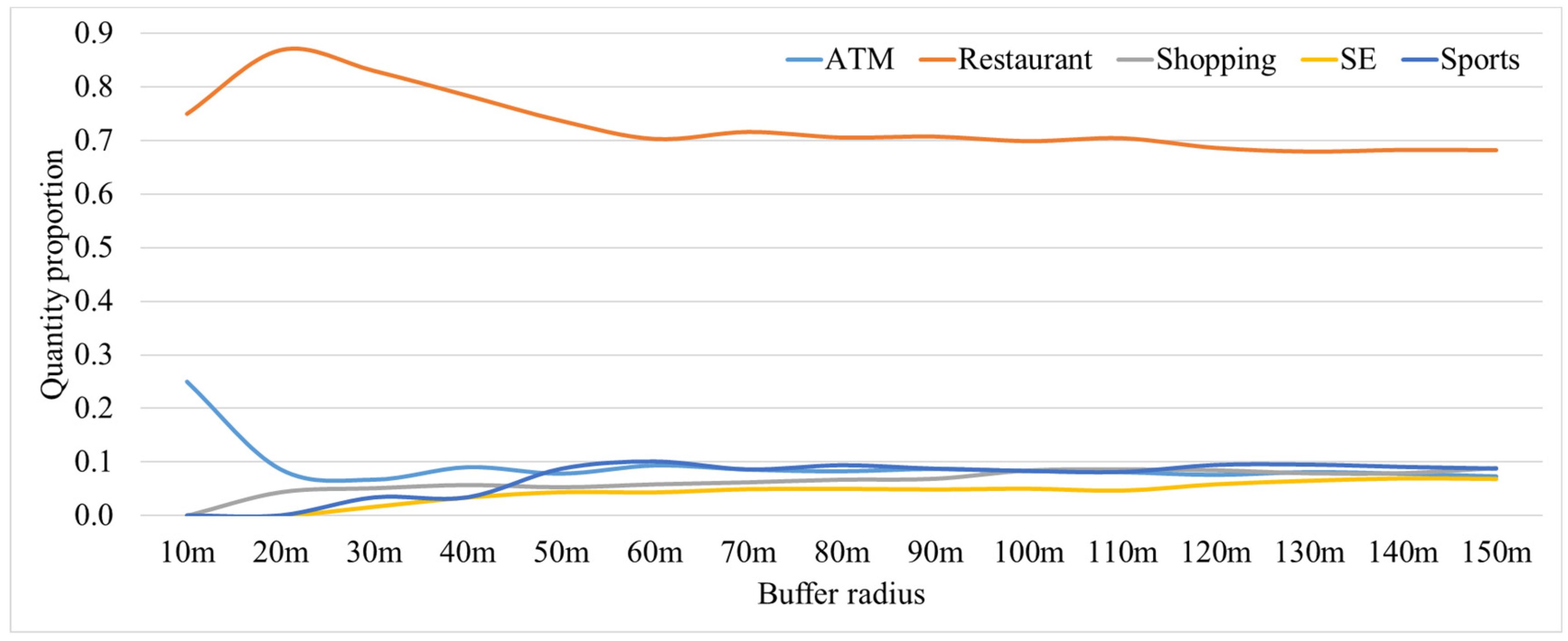
Figure 10 shows five individual verification trajectories with 117 verification access points near the anchor points (s [10 September 2022 7:20:00], e [10 September 2022 8:50:00]). The access point only contains coordinate information and time information, without specific place name information, so the POI near the access point is likely to be accessed. Considering that buildings and roads have a certain width, we count the number of POI points within a buffer of 10~150 m of access points. We found that the quantity proportion of various POIs tended to stabilize after 60 m (Figure 11). Therefore, we built a 60 m buffer for the access points and counted the frequency of each POI contained within the buffer. This frequency will serve as the real distribution of the access probability of POI position points being accessed.

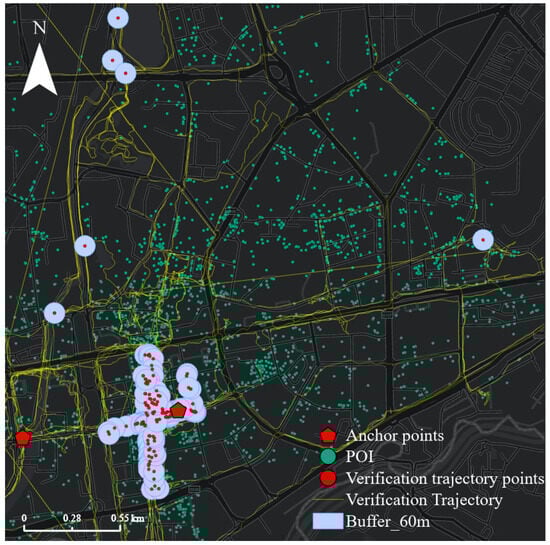
Figure 10. Individual trajectory data.

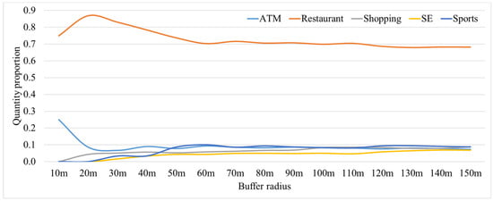
Figure 11. Quantity proportion of POIs in buffer.

As indicated above, each POI position point has three probability values: the position probability calculated using TGDE, the access probability calculated using the model in this paper, and the real access probability generated through trajectory data statistics. In cases where individual trajectory data is limited, 138 POI position points have all three probability values. Thus, two $RMSE\mathrm{s}$ can be calculated for each POI, namely ${RMSE}_{TGDE\_REAL}$ and ${RMSE}_{NEW\_REAL}$, and ${RMSE}_{TGDE\_REAL}$ represents the $RMSE$ between the theoretical value calculated using the classical TGDE model and the real access probability value. ${RMSE}_{NEW\_REAL}$ represents the $RMSE$ between the theoretical value calculated using the “Mutual feedback model” and the real access probability value.

In order to more intuitively visualize the prediction effect of the two models, we calculate ${RMSE}_{TGDE\_REAL}-{RMSE}_{NEW\_REAL}$, and the value is positive, so the prediction of the model in this paper is more accurate. If the value is negative, TGDE prediction is more accurate. If the value is 0, the two models have the same prediction effect. As can be seen from Figure 12, 89 POIs:${RMSE}_{TGDE\_REAL}-{RMSE}_{NEW\_REAL}>0$, and 49 POIs:${RMSE}_{TGDE\_REAL}-{RMSE}_{NEW\_REAL}<0$. Therefore, the “Mutual feedback model” proposed in this paper is more reasonable compared to the classical TGDE model.

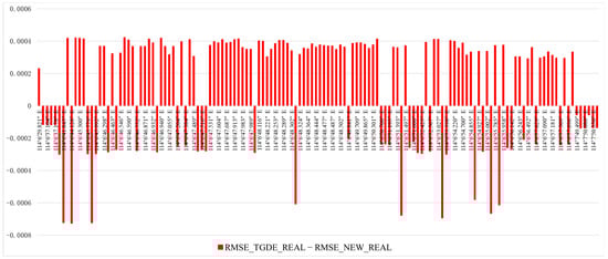
Figure 12. Model prediction effect.

In order to verify the influence of type weights on the accuracy of the model, we treat all POIs as sample points and set the current type weights as Type Weight I (0.15, 0.4, 0.15, 0.15, 0.15) and Type Weight II (0.05, 0.5, 0.05, 0.3, 0.1). The $RMSE\mathrm{s}$ between the theoretical value calculated using the model in this paper and the real access probability value are 0.001663 and 0.001657, respectively. It is found that, on the basis of following the size relationship between the type weights, changing the value of the type weights has little impact on the results, but it has an impact on the access probability of a single POI position point (Figure 13). The above conclusions also show that although the amount of individual trajectory data is limited, and the difference between people’s living habits in different regions leads to different time distributions of the change of access probability, these factors generally have little impact on the framework of the model proposed in this paper. When applied to different cities in the future, the POI-type weight value can be dynamically adjusted accordingly.

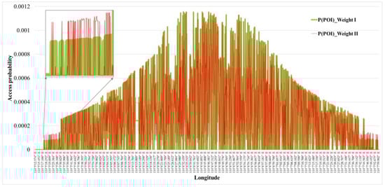
Figure 13. Changes in POI access probability distribution before and after type weight changes.

5. Discussion

The model proposed in this paper is inclined to be theoretical, and future work should discuss the applicability of the model proposed regarding the study of people, vehicles, or other moving objects and its application to urban road network space. Individual activity trajectory data provide data support for the construction of smart cities and the analysis of human activity rules. However, data obtained through interviews or questionnaires are generally missing, either because of the decline in individual memory or because of privacy concerns. Modern positioning technology can provide relatively accurate position information, but it cannot characterize individual activity and cannot express position information for individuals who are not wearing locatable electronic devices. Therefore, the practicability of individual activity trajectory data will be limited. Data deficiency is a serious problem in the context of big data. However, with the development of modern positioning technology, multi-object trajectory space–time big data has become easy to obtain. The definition of the space–time influence range of moving objects has been widely used in many scenarios, such as public health, the service industry, and transportation.

The method proposed in this paper can predict the space–time uncertainty of an individual moving object accessing POI position points between known trajectory points. This uncertainty is quantitatively described in a probabilistic way, so as to complete the space–time information of individual activities to the greatest extent, which can provide new ideas for epidemic prevention and control, tracking and arresting criminals, searching for missing persons, and other scenarios.

In epidemic prevention and control, patients’ epidemiological survey trajectory information is usually discontinuous. The model proposed in this paper can use the limited trajectory information to evaluate the access probability of patient activity space and assist the epidemic risk assessment in the region without footprint records. In this way, the space–time trajectory information of patients’ activities is restored as comprehensively as possible, which provides technical support for identifying and screening close contacts and effectively preventing and controlling the epidemic.

During the process of criminals being arrested by the police, criminals may intentionally hide, and the tracking information typically provided by witnesses and surveillance is often incomplete. The method proposed in this paper makes use of the principle of time geography, and through part of the trajectory information, it can infer the position points that criminals may access with high probability, which provides a reference for police deployment and thus improves the efficiency of criminal arrest.

Similarly, in the process of searching for missing persons, it is very difficult to obtain detailed trajectory information about missing persons, and the search and rescue work for missing persons must be fast and efficient. The method proposed in this paper can effectively reduce the position areas that missing persons may access, improve the utilization rate of search and rescue resources, and thus find the missing persons in the shortest time.

6. Conclusions

Based on the principle of time geography, this paper constructs a probabilistic time geography model, also known as the Mutual feedback model, which considers POI semantics. The method of estimating POI access probability proposed in this paper can quantitatively measure the uncertainty of each POI position point being accessed within an individual’s potential activity range through the space–time information of trajectory points. This method establishes the mapping relationship and mathematical model between space–time trajectory points and POI position points and analyzes all the information of individuals accessing uncertain position points between known trajectory points, such as individual activity time, POI opening time and minimum service time, space–time distance cost, and POI type. The method proposed in this paper is helpful in supplementing and perfecting the theoretical system of time geography research.

References

- Winter, S. Towards a Probabilistic Time Geography. In Proceedings of the 17th ACM SIGSPATIAL International Conference on Advances in Geographic Information Systems, Washinghton, DC, USA, 4–6 November 2009; pp. 528–531. [Google Scholar] [CrossRef]
- Downs, J.A. Time-geographic density estimation for moving point objects; Lecture Notes in Computer Science (including subseries Lecture Notes in Artificial Intelligence and Lecture Notes in Bioinformatics). In Geographic Information Science: 6th International Conference, GIScience 2010, Zurich, Switzerland, 14–17 September 2010; Springer: Berlin/Heidelberg, Germany, 2010; pp. 16–26. [Google Scholar] [CrossRef]
- Downs, J.; Horner, M.; Lamb, D.; Loraamm, R.W.; Anderson, J.; Wood, B. Testing time-geographic density estimation for home range analysis using an agent-based model of animal movement. Int. J. Geogr. Inf. Sci. IJGIS 2018, 32, 1505–1522. [Google Scholar] [CrossRef]
- Yin, Z.C.; Wu, Y.; Winter, S.; Hu, L.F.; Huang, J.J. Random encounters in probabilistic time geography. Int. J. Geogr. Inf. Sci. IJGIS 2018, 32, 1026–1042. [Google Scholar] [CrossRef]
- Downs, J.A.; Horner, M.W. Adaptive-Velocity Time-Geographic Density Estimation for Mapping the Potential and Probable Locations of Mobile Objects. Environ. Plan. B Urban Anal. City Sci. 2014, 41, 1006–1021. [Google Scholar] [CrossRef]
- Miller, H.J. Necessary Space-Time Conditions for Human Interaction. Environ. Plan. B Urban Anal. City Sci. 2005, 32, 381–401. [Google Scholar] [CrossRef]
- Yin, Z.; Huang, K.; Ying, S.; Huang, W.; Kang, Z. Modeling of Time Geographical Kernel Density Function under Network Constraints. ISPRS Int. J. Geo-Inf. 2022, 11, 184. [Google Scholar] [CrossRef]
- Hägerstrand, T. What about People in Regional Science? Pap. Reg. Sci. Assoc. 1970, 24, 6–21. [Google Scholar] [CrossRef]
- Lenntorp, B. Time-geography —At the end of its beginning. GeoJournal 1999, 48, 155–158. [Google Scholar] [CrossRef]
- Shaw, S.-L.; Yu, H. A GIS-based time-geographic approach of studying individual activities and interactions in a hybrid physical–virtual space. J. Transp. Geogr. 2009, 17, 141–149. [Google Scholar] [CrossRef]
- Shaw, S. Guest editorial introduction: Time geography—Its past, present and future. J. Transp. Geogr. 2012, 23, 1–4. [Google Scholar] [CrossRef]
- Miller, H.J. A measurement theory for time geography. Geogr. Anal. 2005, 37, 17–45. [Google Scholar] [CrossRef]
- Long, J.; Nelson, T. Home range and habitat analysis using dynamic time geography. J. Wildl. Manag. 2015, 79, 481–490. [Google Scholar] [CrossRef]
- Elias, D.; Kuijpers, B. A note on measuring the volume of space-time prisms and the area of their spatial projections. Trans. GIS 2020, 24, 1427–1436. [Google Scholar] [CrossRef]
- Demšar, U.; Long, J.A. Potential path volume (PPV): A geometric estimator for space use in 3D. Mov. Ecol. 2019, 7, 14. [Google Scholar] [CrossRef] [PubMed]
- Winter, S.; Yin, Z.C. Directed movements in probabilistic time geography. Int. J. Geogr. Inf. Sci. IJGIS 2010, 24, 1349–1365. [Google Scholar] [CrossRef]
- Downs, J.A.; Lamb, D.; Hyzer, G.; Loraamm, R.; Smith, Z.J.; O’Neal, B.M. Quantifying spatio-temporal interactions of animals using probabilistic space–time prisms. Appl. Geogr. 2014, 55, 1–8. [Google Scholar] [CrossRef]
- Downs, J.A.; Horner, M.W.; Hyzer, G.; Lamb, D.; Loraamm, R. Voxel-based probabilistic space-time prisms for analysing animal movements and habitat use. Int. J. Geogr. Inf. Sci. IJGIS 2014, 28, 875–890. [Google Scholar] [CrossRef]
- Song, Y.; Miller, H.J. Simulating Visit Probability Distributions within Planar Space-Time Prisms. Int. J. Geogr. Inf. Sci. IJGIS 2014, 28, 104–125. [Google Scholar] [CrossRef]
- Long, J.A.; Nelson, T.A.; Nathoo, F.S. Toward a kinetic-based probabilistic time geography. Int. J. Geogr. Inf. Sci. IJGIS 2014, 28, 855–874. [Google Scholar] [CrossRef]
- You, Q.; Krumm, J. Transit Tomography Using Probabilistic Time Geography: Planning Routes without a Road Map; Taylor & Francis, Inc.: Abingdon, UK, 2014. [Google Scholar] [CrossRef]
- Liu, Y.; Seah, H.S. Points of interest recommendation from GPS trajectories. Int. J. Geogr. Inf. Sci. IJGIS 2015, 29, 953–979. [Google Scholar] [CrossRef]
- Milias, V.; Psyllidis, A. Assessing the influence of point-of-interest features on the classification of place categories. Comput. Environ. Urban Syst. 2021, 86, 101597. [Google Scholar] [CrossRef]
- Jiao, X.; Xiao, Y.; Zheng, W.; Wang, H.; Hsu, C.H. A novel next new point-of-interest recommendation system based on simulated user travel decision-making process. Future Gener. Comput. Syst. 2019, 100, 982–993. [Google Scholar] [CrossRef]
- Bui, T. Automatic construction of POI address lists at city streets from geo-tagged photos and web data: A case study of San Jose City. Multimed. Tools Appl. 2023, 82, 34749–34770. [Google Scholar] [CrossRef]
- Jiao, H.; Xiao, M. Delineating Urban Community Life Circles for Large Chinese Cities Based on Mobile Phone Data and POI Data—The Case of Wuhan. ISPRS Int. J. Geo-Inf. 2022, 11, 548. [Google Scholar] [CrossRef]
- Zheng, D.; Li, C. Research on Spatial Pattern and Its Industrial Distribution of Commercial Space in Mianyang Based on POI Data. J. Data Anal. Inf. Process. 2020, 8, 20–40. [Google Scholar] [CrossRef]
- Lim, N.; Hooi, B.; Ng, S.-K.; Goh, Y.L.; Weng, R.; Tan, R. Hierarchical Multi-Task Graph Recurrent Network for Next POI Recommendation. In Proceedings of the 45th International ACM SIGIR Conference on Research and Development in Information Retrieval, Madrid, Spain, 11–15 July 2022. [Google Scholar] [CrossRef]
- Yin, H.; Cui, B.; Zhou, X.; Wang, W.; Huang, Z.; Sadiq, S. Joint Modeling of User Check-in Behaviors for Real-time Point-of-Interest Recommendation. ACM Trans. Inf. Syst. 2017, 35, 1–44. [Google Scholar] [CrossRef]
- Kan, Z.; Kwan, M.P.; Liu, D.; Tang, L.; Chen, Y.; Fang, M. Assessing individual activity-related exposures to traffic congestion using GPS trajectory data. J. Transp. Geogr. 2022, 98, 103240. [Google Scholar] [CrossRef]
- Zeng, L.; Liu, Y.; Qing, R.; Zhong, K.; Liu, M.; Liao, Z.; Zhao, Y. Study on the Change of POI Attraction Based on Taxi Trajectory; Lecture Notes on Data Engineering and Communications Technologies. In Advances in Intelligent Automation and Soft Computing; Springer International Publishin: New York, NY, USA, 2022; pp. 102–110. [Google Scholar] [CrossRef]
- Borruso, G. Network Density Estimation: A GIS Approach for Analysing Point Patterns in a Network Space. Trans. GIS 2008, 12, 377–402. [Google Scholar] [CrossRef]
- Li, Q.; Zhang, T.; Wang, H.; Zeng, Z. Dynamic accessibility mapping using floating car data: A network-constrained density estimation approach. J. Transp. Geogr. 2011, 19, 379–393. [Google Scholar] [CrossRef]
- Downs, J.A.; Horner, M.W. Probabilistic potential path trees for visualizing and analyzing vehicle tracking data. J. Transp. Geogr. 2012, 23, 72–80. [Google Scholar] [CrossRef]
- Ermagun, A.; Fan, Y.; Wolfson, J.; Adomavicius, G.; Das, K. Real-time trip purpose prediction using online location-based search and discovery services. Transp. Res. Part C Emerg. Technol. 2017, 77, 96–112. [Google Scholar] [CrossRef]
- Hodson, T.O. Root-mean-square error (RMSE) or mean absolute error (MAE): When to use them or not. Geosci. Model Dev. 2022, 14, 5481–5487. [Google Scholar] [CrossRef]
Disclaimer/Publisher’s Note: The statements, opinions and data contained in all publications are solely those of the individual author(s) and contributor(s) and not of MDPI and/or the editor(s). MDPI and/or the editor(s) disclaim responsibility for any injury to people or property resulting from any ideas, methods, instructions or products referred to in the content. |
© 2024 by the authors. Licensee MDPI, Basel, Switzerland. This article is an open access article distributed under the terms and conditions of the Creative Commons Attribution (CC BY) license (https://creativecommons.org/licenses/by/4.0/).