Efficient Trajectory Clustering with Road Network Constraints Based on Spatiotemporal Buffering

Abstract

The analysis of individuals’ movement behaviors is an important area of research in geographic information sciences, with broad applications in smart mobility and transportation systems. Recent advances in information and communication technologies have enabled the collection of vast amounts of mobility data for investigating movement behaviors using trajectory data mining techniques. Trajectory clustering is one commonly used method, but most existing methods require a complete similarity matrix to quantify the similarities among users’ trajectories in the dataset. This creates a significant computational overhead for large datasets with many user trajectories. To address this complexity, an efficient clustering-based method for network constraint trajectories is proposed, which can help with transportation planning and reduce traffic congestion on roads. The proposed algorithm is based on spatiotemporal buffering and overlapping operations and involves the following steps: (i) Trajectory preprocessing, which uses an efficient map-matching algorithm to match trajectory points to the road network. (ii) Trajectory segmentation, where a Compressed Linear Reference (CLR) technique is used to convert the discrete 3D trajectories to 2D CLR space. (iii) Spatiotemporal proximity analysis, which calculates a partial similarity matrix using the Longest Common Subsequence similarity indicator in CLR space. (iv) Trajectory clustering, which uses density-based and hierarchical clustering approaches to cluster the trajectories. To verify the proposed clustering-based method, a case study is carried out using real trajectories from the GeoLife project of Microsoft Research Asia. The case study results demonstrate the effectiveness and efficiency of the proposed method compared with other state-of-the-art clustering-based methods.

1. Introduction

Recent technological advancements have made it possible to collect large amounts of data on the movement patterns of people [1], vehicles [2], and animals. These data can be collected through sensors such as the global system for mobile communications (GSM), the global positioning system (GPS), and the Wi-Fi found in smartphones and cars, and it is useful in transportation planning to understand travel behavior [3], which can be grouped into patterns or clusters [4]. Data mining techniques, such as classification, clustering, and association rule mining, are used to analyze data and find valuable patterns related to time and space [5]. Clustering is used to group similar data points based on their characteristics. In the case of trajectory data, this means grouping together sets of spatiotemporal data points (i.e., location and time) with similar movement patterns. For example, clustering vehicle trajectory data can reveal patterns of rush hour traffic or common routes taken by vehicles [6].

Trajectory clustering allows researchers to discover information about the movement patterns of people, animals, and vehicles that would not be easily observable from individual data points [7]. By grouping similar data, researchers can identify patterns and trends in the data that would otherwise be difficult to detect. Additionally, trajectory clustering can also be used to extract meaning from the data. For example, by identifying movement patterns, researchers can gain insights into how people, animals, or vehicles use a particular area, such as which routes they prefer or which areas they avoid [8]. This information can then be used to make informed decisions, such as in transportation planning, where it can be used to optimize infrastructure and reduce traffic congestion.

However, calculating the similarity between trajectories is a challenging task, as different trajectories have different lengths and sampling frequencies. Researchers often use Longest Common Subsequence (LCSS) [9] and Dynamic Time Warping (DTW) [10] to calculate the similarity between unequal-length trajectories, but this can be time-consuming. In addition to that, the principle of minimum total curvature techniques is used for 2D interpolation of geophysical data in order to generate maps using a computer, which may not always be perfect but are generally sufficient to analyze a spatially distributed data [11]. Ridge regression, proposed by [12], can be used to estimate the coefficients for a linear model that predicts the similarity between two trajectories based on their features or attributes. Moreover, the authors of a study on Polish urban areas, as cited in [13], discussed the challenges involved in sustainable transport development and offered potential solutions to mitigate short-term and long-term adverse impacts on urbanization.

In trajectory compression, the trajectory clustering method reduces the consumption of computing and storage resources for trajectory data mining. Trajectory similarity measurement is the central part of the trajectory clustering algorithms. Before trajectory clustering, the similarity or distance of two distinguished trajectory data must be compared. Different similarity measurement methods have been used in further research with their aspects. Some of the methods are used for underlaying the road network space. The Euclidean distance, the similarity measurement method, is no longer suitable for calculating the distance between two points in road network space. Therefore, in the road network space, we use the shortest path of two points to describe the distance between the two points in the road network. Similarity measure methods using the Euclidean distance lead to bad results, mainly because trajectories have different lengths [14]. Different trajectory similarity measurement methods with road network space are also introduced, such as Hausdorff and Frechet distances. They are used for trajectories clustering similarity (distance) measures but fail to compare them as a whole for their high computational cost. Spatial–temporal trajectories are composed of spatial location points with time information. Different trajectories have different lengths and sampling frequencies. Therefore, the method suitable for calculating the similarity between trajectories of equal length, such as average of pair distance (APD), is no longer applicable. In previous articles, researchers often used LCSS and DTW to calculate the similarity between unequal-length trajectories, because the distance calculation of the road network is time-consuming, and most of the similarity calculations of spacetime trajectories, such as LCSS, require calculating the shortest path between each spacetime point to obtain the similarity between the spacetime trajectories. This needs to be more efficient in the era of big data. Our main goal of this research is to provide an efficient cluster of the trajectories in the network space, because this trajectory clustering in the road network space in the traditional method could be more efficient. Here, we introduce a novel method in which we construct similarity measures using spatiotemporal proximity analysis with LCSS.

Map matching, a preprocessing step, is needed to map each point in a road network route. Above all, concentrating just on the available vehicle trajectory data is tremendously detrimental if the associated network structure is not prepared. In this study, we focus on the clustering problem and its eventual resolution, which calls for an understanding of the underlying road network. In developing a similarity measure, we take into account that there exist road network limits for vehicle movements even if our goal is to map trajectories to known road segments. We assume that trajectories on the same route overlap due to the network constraint (at a macroscopic scale). This helps in locating the LCSS between two portions when using the method. To assess the proximity, compatibility, and amount of synchronization between two trajectories, we analyze how near they overlap. This computation of similarity based on the LCSS is conceptually equivalent to the shortest route for fully network-mapped items and the network distance for free-moving objects. On the other side, to enhance over time computation to identify the similarity, we use the spatiotemporal buffering approach. The cluster of comparable trajectories is then created using two clustering techniques: hierarchical clustering and density-based clustering.

The main objective of this research is to provide efficient clustering-based trajectories in the network space. Most existing methods require a complete similarity matrix to quantify the similarities among users’ trajectories in the dataset [15]. The size of such a similarity matrix increases exponentially with the number of users in the trajectory dataset, leading to significant computational overhead.

The main challenge with trajectory clustering is the significant computational overhead required to calculate the similarity matrix for a big dataset with many user trajectories. This becomes even more severe for network constraint trajectories, which require additional shortest-path calculations to calculate trajectory similarities in road networks. As a result, most existing methods can perform the clustering analysis only for a tiny dataset of network constraint trajectories. Therefore, efficiently performing clustering analysis for network constraint trajectories is a critical problem that needs to be solved, given the explosive growth of network constraint trajectory data in real-time applications.

The main contributions of this work are threefold:

• We propose a method to speed up region queries in DBSCAN and reduce the time complexity to generate the cluster.
• Our proposed method uses a network-constrained spacetime path with a spacetime buffer and network spacetime buffer in CLR space.
• We describe the proposed density-based clustering algorithm to overcome the time complexity and speed up the region query.

The remainder of the paper is structured as follows. Section 2 presents a literature review of existing clustering algorithms and similarity measures for moving objects. Section 3 describes the problem that the research aims to address, which is the inefficiency of existing methods for calculating the similarity between trajectories of different lengths Section 4 introduces the density-based spatiotemporal proximal analysis method, which is used to construct similarity measures for spatiotemporal data. The density-based clustering algorithm, which utilizes the method from Section 4, is presented in Section 5. In Section 6, the process of data preparation and preprocessing is discussed. The effectiveness of the proposed methods is evaluated through experiments on trajectory data in Section 7. Finally, in Section 8, we conclude the findings of this study.

2. Literature Review

There are three main domains of research in the field of movement data analysis that involve trajectory clustering: time geography, moving object databases, and the quantitative data analysis method for movement [16]. Many clustering methods have been proposed throughout the years that can be used in trajectory clustering. The key elements in trajectory clustering analysis are cluster algorithms and similarity measures [16]. Yuan et al. [17] presented a review on the development and trends of moving objects clustering algorithms. Yuan et al. [17] and Han et al. [18] presented clustering algorithms in five categories, including partitioning methods, hierarchical methods (e.g., BIRCH), density-based methods (e.g., DBSCAN), grid-based methods (e.g., STING), and model-based clustering algorithms.

Partition-based methods divide the trajectory dataset into a predetermined number of clusters and assign each trajectory to the cluster with the closest centroid, e.g., k-means and k-medoids [19]. Hierarchical-based algorithms build a hierarchy of clusters, where each cluster is formed by merging two or more smaller clusters [18]. They are simple, but they can be difficult to use because it is not always clear whether to combine or split points. These are further divided into three types [20]: bottom-up or condensation algorithms [21], top-down or decomposition algorithms [22], and compound algorithms [23]. On the other hand, density-based clustering algorithms group data points that are densely packed together and separated from other points by a low-density region. These algorithms can handle clusters of any shape, unlike distance-based clustering algorithms, which can only handle spherical clusters [24]. Examples of density-based clustering algorithms include DBSCAN (Density-Based Spatial Clustering of Applications with Noise) and OPTICS (Ordering Points To Identify the Clustering Structure) [24].

Grid-based clustering techniques employ a multiresolution grid data structure to quantize the data space into a grid structure. On the grid, clustering is done, and the effectiveness of the clustering is based on how well the data is compressed there. These algorithms execute quickly and only rely on the number of cells in each dimension of the quantized space; processing time is independent of the quantity of data points. STING (STatistical INformation Grid) and CLIQUE (CLustering In QUEst) are two examples of grid-based clustering algorithms [25].

Model-based clustering algorithms use statistical models to describe the data and cluster the data according to the model [26]. Examples of model-based clustering algorithms include Gaussian mixture models and hidden Markov models.

Each of these algorithms have their own strengths and weaknesses. The use of them depends on the problem statement and requirements of the users. Several similarity measures have been proposed to determine the similarity between two trajectories and can be used as the basis of clustering algorithms. Some of the common similarity measures are Euclidean distance, DTW, Frechet distance, Hausdorff distance, and LCSS [17].

Euclidean distance calculates the straight-line distance between two points in space. It can be used to calculate the distance between two trajectories by summing the distances between corresponding points on the two trajectories [27]. However, DTW calculates the similarity between two time series by aligning the time points of the series and minimizing the accumulated distance between them. It is often used for trajectory clustering because it is able to handle variations in speed and direction [28]. Frechet distance calculates the minimum distance required to travel from one trajectory to another, taking into account the path and order of the points on the trajectories. It is often used for trajectory clustering because it is able to handle nonlinear movements [29].

Hausdorff distance calculates the maximum distance between two trajectories and is often used for trajectory clustering because it is able to handle large variations in shape [30], and LCSS calculates the similarity between two sequences by identifying the LCSS shared by the two sequences. It is often used for trajectory clustering because it is able to handle variations in the order of the points on the trajectories [31].

This study addresses trajectory clustering without road network information. Although we do map trajectories to known road segments, while creating a similarity measure we take into consideration the fact that vehicle movements are limited by the road network. To be more specific, we gauge the degree of overlap between two trajectories to gauge how similar they are to one another by assuming that trajectories on the same direction entirely overlap at a macroscopic size. This method sits between between the shortest route for completely network-mapped items and the network distance for freely moving objects. To improve the efficiency of our similarity calculation over time, we utilize the spatiotemporal buffering technique. After calculating the similarity between trajectories using LCSS, we use hierarchical and density-based clustering to similarly group trajectories into clusters. This approach does not require the nontrivial effort of map matching, which is the process of mapping each point in a road network route to the corresponding network topology.

3. Problem Statement

Figure 1 illustrates the research method proposed in this research to address the clustering-based trajectories problem. The proposed method constructs similarity measures using spatiotemporal proximity analysis (SP-Analysis) [16] with LCSS.

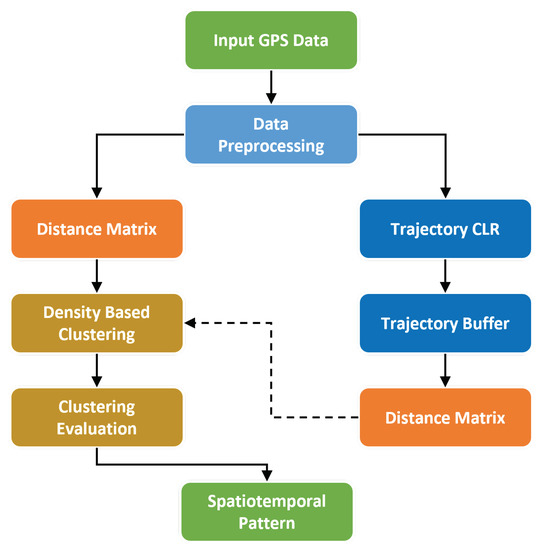
Figure 1. Overall framework of our proposed trajectory clustering method.

In spatially organized road networks e.g., $(x,y,t)$ space, individuals cannot travel freely in metropolitan regions. A directed graph, $G=(N,A)$, may be used to model a road network. $mathrmN$ and $mathrmA$ represent the nodes and connections, respectively. Each link, $a_u\in A$, has a unique set of properties, such as the link identity, $l_u$, travel time, $t_u$, and link length, $d_u$. A link, $a_u$, is made up of a beginning node $n_s^u$, an ending node $n_e^u$, and a collection of intermediate vertices $n_i^u$. According to a set of linked segments that join each of the link’s two neighboring vertices, the geometry of the connection may be characterized (See Figure 2).

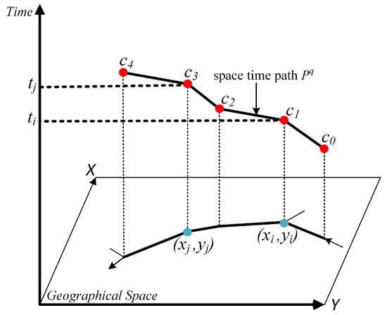
Figure 2. Spacetime route in $(x,y,t)$ limited by the network.

As a collection of control points and route segments in a road network, a network-constrained spacetime path $P^q$ may be seen. For the road network to retain its route topology, control points should offer both observations and network nodes. The individual position at any $t_k\in \left[t_i,t_j\right]$ using the linear interpolation is $P^q\left(t_k\right)$ can be computed as

$$P^q\left(t_k\right)=\left\{\left(l_u,m_k,t_k\right)\mid m_k=(1-\lambda )m_i+\lambda m_j;\lambda =\left(t_k-t_i\right)/\left(t_j-t_i\right)\right\}$$

(1)

where $m_i\in (0,1)$ is the location’s relative position on link $a_u$.

The similarity distance metric is one of the clustering algorithm’s most important components. The similarity or distance between two different trajectory data must be assessed before they can be grouped into clusters. According to their necessity for usage, multiple similarity measure metrics exist; some are appropriate for varying durations of trajectories.

With the constraint of the shortest path across the road network, several definitions of the similarity of trajectories (such as destination-based, origin-based, route-based, etc.) may be made in traffic analysis. While the movement of trajectories is restricted by the road network, one method is to look at whether the two trajectories overlap or intersect; if they traveled the same piece of the route, parts of trajectories would be fully overlapping (at a macroscopic scale). We calculate the similarity distance between the trajectories and the overlapping portions of the trajectories using the LCSS technique. The longest possible subsequence of two trajectories may be found using the LCSS technique, which was developed in the related string domain. Two strings of varying lengths are provided, and the goal is to identify a collection of strings that appear in both strings from left to right. By allowing two sequences to extend without changing the series of components yet allowing certain elements to be mismatched, the LCSS model can match two sequences [32]. Many research have also used the LCSS technique in the context of trajectory clustering. Typically, the LCSS is solved recursively. The shortest distance is defined as NTdist if it is smaller than the provided distance threshold and the time threshold between two network points of trajectories;

$$\begin{array}{c}\hfill LCSS\left(p_n^i,q_m^j\right)=\{0\mathrm{if}m=n=0LCSS(Rest\left(p\right),Rest\left(q\right))+1\mathrm{NTdist}\le \\ \hfill \epsilon max\{LCSS(Rest\left(p\right),q)LCSS(p,Rest\left(q\right)\left)\right\}\mathrm{otherwise}\end{array}$$

(2)

The LCSS between two trajectory segments $p^i$ and $q^j$, whose lengths are $n$ and $m$, is $LCSS\left(p_n^i,q_m^j\right)$. A pair of trajectory points are deemed similar and the LCSS value is raised by 1 when the network distance between two trajectories $mathrmA$ and $mathrmB$ is smaller than the specified threshold. $LCSS\left(p_n^i,q_m^j\right)=0$ if the number of points of trajectories equals $mathrmn$ and $mathrmm$ is 0. The highest common subsequence may be determined iteratively if the points of both trajectories are not 0.

The two user-provided input parameters used in density-based clustering determine the number of clusters. These two input parameters are $\epsilon$ and $MinTras$, where the former specifies the neighborhood’s minimal similarity and the latter describes the minimum number of neighbors that the trajectory must have in order to be considered as the core object within the given range. All of the trajectories in the vicinity of the core object are edge objects, while the other trajectories are noise objects. Using the LCSS, the distance between trajectories is determined by comparing how similar they are. The LCSS operation is used to assess the $\epsilon$-neighbourhood of the trajectory $T{r}_i$ that is indicated by $N_{\epsilon }\left(T{r}_i\right)$ to find the trajectory whose corresponding similarity value is higher than 0. Moreover, we discover that a trajectory’s $\epsilon$-neighbourhood is the trajectory whose similarity value is bigger than $\epsilon$. If $T{r}_j\in N_{\epsilon }\left(T{r}_i\right)$ and $\left|N_{\epsilon }\left(T{r}_i\right)\right|\ge MinTras$, which is a fundamental need for a trajectory, then $T{r}_j$ is directly density-reachable from $T{r}_i$. If there is a chain of trajectories $T{r}_i,\dots ,T{r}_n,T{r}_{n+1},\dots ,T{r}_j$ such that the $T{r}_{n+1}$ is directly density-reachable from $T{r}_n$, then all trajectories in the chain must be core trajectories, with the potential exception of $T{r}_j$. If there is a trajectory $T{r}_i$ and both $T{r}_j$ and $T{r}_k$ are density-reachable from $T{r}_i$ in terms of $\epsilon$ and $MinTras$, then a trajectory $T{r}_j$ and a trajectory $T{r}_k$ are density-connected to one another.

Most proposed methods require computing a complete similarity matrix to measure the similarities between the trajectories of all users in the dataset. However, with the number of users in the trajectory dataset, the size of such a similarity matrix increases exponentially. This results in significant computational overhead when calculating the similarity matrix for a large dataset with many user trajectories. This overhead computation is even more severe for trajectories of network constraints, in which additional shortest-path calculations are needed to measure trajectory similarities in road networks. Consequently, most current approaches can only perform clustering analysis for a small dataset of trajectories of network constraint. Therefore, efficiently implementing clustering analysis for trajectories of network constraints becomes an urgent problem to solve, given the exponential growth of network constraint trajectory data in real applications.

4. Density-Based Spatiotemporal Proximal Analysis

The proposed density-based clustering algorithm is developed based on spatiotemporal buffering and overlapping operations. So, first, we need the spatiotemporal buffering on the network constraint. The proximal spatiotemporal trajectories in network distance can be effectively calculated to determine their similarities for a provided trajectory. In contrast, the similarity calculation can neglect other trajectories with large spatiotemporal distances.

4.1. Spatiotemporal Buffer on the Network Constraint

The process of continually building forward $A_k^f\left(\omega \right)$ and backward $A_k^b\left(\omega \right)$ spatial buffers for every $P^q\left(t_k\right)$ along the journey across the road network results in the network spacetime buffer $ST{B}^q\left(\omega \right)$. Network locations produce a forward spatial buffer defined by $A_k^f\left(\omega \right)$ by meeting the starting condition. The shortest forward route search may be used to determine this buffer using $P^q\left(t_k\right)$ as the node of origin. After satisfying the latter requirement, network sites that constitute a backward spatial buffer are specified by $A_k^b\left(\omega \right)$. This value may be determined by utilizing $P^q\left(t_k\right)$ as the node of destination in the shortest forward route search, as illustrated in Figure 3. Creating the forward and backward spacetime buffers, $ST{B}_{ij}^f\left(\omega \right)$ and $ST{B}_{ij}^b\left(\omega \right)$, only requires the forward and backward spatial buffers for $s_{ij}^q$ at two control points, $P^q\left(t_i\right)$ and $P^q\left(t_j\right)$. The network spacetime buffer can be accurately generated after $ST{B}_{ij}^f\left(\omega \right)$ and $ST{B}_{ij}^b\left(\omega \right)$ are generated for any segment of spacetime path $\forall s_{ij}^q\in P^q$. The constructed $ST{B}^q\left(\omega \right)=ST{B}_{ij}^f\left(\omega \right)\cup ST{B}_{ij}^b\left(\omega \right)$. A composed set of polygons upon the link generated as $ST{B}^q\left(\omega \right)=<\cdots ,O_u^q,\dots >$, where $O_u^q$ shows the spacetime polygon over the link $a_u$ [16].

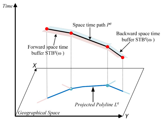
Figure 3. Network-constrained spacetime path with spacetime buffer in $(x,y,t)$ space.

4.2. Spatiotemporal Analysis in CLR Space

We manage the shifting object indexes using the Compressed Linear Reference (CLR) [33] approach and convert 3D road network-constrained time geographic entities in $(x,y,t)$ space to $2\mathrm{D}$ entities in CLR space. The link identity $l_i$ is the link identity, a distinct positive integer number, integrated into a single real value $z_i^u=l_u,m_i$. The linear reference $\left(l_u,m_i\right)$ is an analogous one-to-one representation of geographical position $\left(x_i,y_i\right)$ in the road network. The $z_i^u$ value may be readily converted to a location using dynamic subdivision and is also identical to $\left(x_i,y_i\right)$ in $2\mathrm{D}$. Every $3\mathrm{D}$ point in the road network may thus be represented as a singular 2D point ${\tilde{c}}_i^u=\left(z_i,t_i\right)$ in $(z,t)$ space, also known as the CLR space.

The spacetime path is transformed in CLR space as ${\tilde{P}}^q$. It comprises a set of disjoint elements of LineString that is polyline $<\cdots ,{\tilde{R}}_u^q,\cdots >$, each line string of a set of disjoint elements corresponding to $R_u^q$ in $(x,y,t)$ in 3D space, representing the continuous movement of an individual on a particular link. A set of segments $<\cdots ,{\tilde{s}}_{ij},\cdots >$ is a collection of further LineString ${\tilde{R}}_u^q$, where each segment $s_{ij}$ in the set is a straight line in CLR space that is connecting two sequential control points ${\tilde{c}}_i^u=\left(z_i,t_i\right)$ and ${\tilde{c}}_j^u=\left(z_j,t_j\right)$ on the same link (See Figure 4).

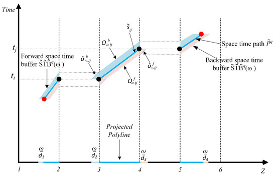
Figure 4. Network spacetime buffer in CLR space (Adapted from [16]).

In CLR space, the network-constrained spacetime path is an equivalent representation of ${\tilde{P}}^q$ in $(x,y,z)$ space [34]. We transform the spacetime buffer by following previous work [34]: $ST{B}^q\left(\omega \right)$ into CLR space by converting spacetime location $c_i^u=$$\left(x_i,y_i,t_i\right)$ to ${\tilde{c}}_i^u=\left(z_i,t_i\right)$. As shown in Figure 4, any $ST{B}^q\left(\omega \right)$ can be transformed by converting each $ST{B}_{ij}^q\left(\omega \right)$ of $s_{ij}^q\in S^q$ into CLR space.

For the path segment $s_{ij}^q$ upon link $a_u,ST{B}_{ij}^q\left(\omega \right)$ is the union of $ST{B}_{ij}^f\left(\omega \right)$ and $ST{B}_{ij}^b\left(\omega \right)$ similarity in the network spacetime path with buffer. Firstly, transform $ST{B}_{ij}^f\left(\omega \right)=<O_{u,ij}^f\left(\omega \right),O_{v,ij}^f\left(\omega \right),\dots >$ into CLR space using different cases. $O_{u,ij}^f\left(\omega \right)$ represent the unique polygon. Thus, ${\mathit{STB}}_{ij}^f\left(\omega \right)=<O_{u,ij}^f\left(\omega \right),O_{v,ij}^f\left(\omega \right),\dots >$ is transformed into unique ${\mathit{STB}}_{ij}^f\left(\omega \right)=<{\tilde{O}}_{u,ij}^f\left(\omega \right),O_{v,ij}^f\left(\omega \right),\dots >$ in CLR space.

Secondly, transform ${\mathit{STB}}_{ij}^b\left(\omega \right)=<O_{u,ij}^b\left(\omega \right),O_{v,ij}^b\left(\omega \right),\dots >$ into CLR space using different cases. $O_{u,ij}^b\left(\omega \right)$ represent the unique polygon. Thus, $ST{B}_{ij}^b\left(\omega \right)=<O_{u,ij}^b\left(\omega \right),O_{v,ij}^b\left(\omega \right),\dots >$ is transformed into unique ${\mathit{STB}}_{ij}^b\left(\omega \right)=<{\tilde{O}}_{u,ij}^b\left(\omega \right),{\tilde{O}}_{v,ij}^b\left(\omega \right),\dots >$ in CLR space.

Unique spacetime buffer in CLR $ST{B}_{ij}^q\left(\omega \right)=ST{B}_{ij}^f\left(\omega \right)\cup ST{B}_{ij}^b\left(\omega \right)$ is transformed by the $ST{B}_{ij}^q\left(\omega \right)=ST{B}_{ij}^f\left(\omega \right)\cup ST{B}_{ij}^b\left(\omega \right)$. The network spacetime buffer $\mathit{STB}{}^q\left(\omega \right)$ in CLR space is an equal representation of ${\mathit{STB}}^q\left(\omega \right)$ in $(x,y,z)$ space.

In CLR space, it is simple to implement the spacetime buffering and overlapping for SP-Analysis of movement data. In the current spatial database, all the spacetime pathways are transformed into CLR space, stored, indexed, and searched as $2\mathrm{D}$ polyline entities (SQLServer). The $2mathrmD$ multipolygon that represents the spacetime route $tildePq$ in CLR space, $S\tilde{T}{\tilde{B}}^q\left(\omega \right)$, is created and represented in CLR space. The complex 3D spatiotemporal searches of buffer—path intersection are immediately implemented by the $2\mathrm{D}$ spatial query, i.e., polygon—polyline intersection in the spatial database.

To efficiently calculate the similarity between spatiotemporal trajectory data and moving object buffers, we use SP-Analysis and LCSS. First, we calculate the distance matrix D between all trajectory data using SP-Analysis. To calculate LCSS for each trajectory, we use the overlapping spacetime operation to reduce computation time. We convert trajectory 3D space into $2\mathrm{D}$ space using CLR and create a buffer with given spatial tolerance along each trajectory. Then, we find the similarity measure between trajectories using spatial–temporal buffer query. We compare the time duration of LCSS, not the number of elements, as we perform similarity analysis on spatiotemporal trajectory data.

5. Proposed Density-Based Clustering Algorithm

The density-based clustering method can well handle the clustering of point sets. Density-Based Spatial Clustering of Applications with Noise (DBSCAN) is a more commonly used clustering method in many applications. The DBSCAN determines the number of clusters according to the two input parameters provided by users. These two input parameters are $\epsilon$ and $MinTras$, where the former specifies the minimum similarity of the neighborhood. At the same time, the latter represents the minimum number of neighbors of the trajectory as the core object (which means trajectory here) in the specified range. The trajectories within the core object’s neighborhood are all edge objects, and the remaining trajectories are noise objects. When the DBSCAN is applied to cluster a spatiotemporal moving object, the objects that need to be clustered are converted from spatial point data to spatiotemporal trajectory data. The similarity calculation between trajectories, such as LCSS, replaces the distance calculation between trajectories. The corresponding input parameters of DBSCAN are the minimum similarity threshold $\epsilon$ and the required number of trajectories $MinTras$ that meet the minimum similarity threshold.

Unlike calculating the distance between point pairs in Euclidean space, the similarity calculation of trajectory data in network space is very time-consuming. In addition to the effect of the trajectory sequence length on the similarity calculation, the calculation of the road network distance, the shortest path, is also more time-consuming than the Euclidean distance. In the original DBSCAN algorithm, the calculation of the similarity matrix between trajectories is often completed by brute-force searching in advance, resulting in inefficiency. Therefore, the SP-Analysis is applied to calculate the similarity.

Based on the above elucidation, the following definitions are given. It should be noted that the following trajectory is a continuous spacetime path with the CLR technique, and the trajectory similarity is calculated using LCSS:

Definition 1. 

ε-neighbourhood of a trajectory.

First, according to the spatiotemporal buffer of trajectory $CL{R}_i$, perform LCSS operation to determine the trajectory whose corresponding similarity value is greater than 0, and then further determine that the trajectory whose similarity value is greater than $\epsilon$ is the $\epsilon$-neighbourhood of a trajectory, denoted by $N_{\epsilon }\left(CL{R}_i\right)$.

Definition 2. 

directly density-reachable.

A trajectory $CL{R}_j$ is directly density-reachable from a trajectory $CL{R}_i$ with respect to $\epsilon$ and $MinClrs$ if

$$CL{R}_i\in N_{\epsilon }\left(CL{R}_i\right)$$

(3)

$$|N_{\epsilon }\left(CL{R}_i\right)|\ge \mathit{MinClrs} (\mathrm{core}\mathrm{object}\mathrm{condition})$$

(4)

Definition 3. 

density-reachable.

If there is a chain of trajectories $CL{R}_i,\dots ,CL{R}_n,CL{R}_{n+1},\dots ,CL{R}_j$ such that $CL{R}_{n+l}$ is directly density-reachable from $CL{R}_{\mu }$, then all of the trajectories in the chain must be the core object with the potential exception of $CL{R}_j$.

Definition 4. 

density-connected.

A trajectory $CL{R}_j$ is density-connected to a trajectory $CL{R}_{\mathcal{s}}$ with respect to $\epsilon$ and MinClrs if there is a trajectory CLR such that both $CL{R}_i$ and $CL{R}_k$ are density reachable from $CL{R}_i$ with respect to $\epsilon$ and $MinClrs$.

According to the above definitions, DBSCAN with SP-Analysis can efficiently generate trajectory data clusters. The trajectory data cluster is the most significant density-connected dataset. In the clustering process, the trajectory data are divided into three types: core object, edge object, and noise object. Core objects are trajectories whose number of $\epsilon$-neighborhood of a trajectory is greater than a given threshold $MinClrs$. Edge objects are trajectories that are directly connected to the core object but are not the core object. The types of trajectories in the trajectory data cluster are either core objects or edge objects. When the core object $CL{R}_i$ is found for the first time, determine whether all trajectory data in $N_c\left(CL{R}_i\right)$ have a trajectory as the core object. If not, determine all trajectories in $N_s\left(CL{R}_i\right)$ as an edge object and add it to the cluster with the core object. If there is, add the trajectory to the cluster and expand the trajectory data cluster by adding its $\epsilon$-neighborhood. The noise object is a trajectory that is neither a core nor an edge object. The specific trajectory clustering algorithm of DBSCAN based on LCSS with SP-Analysis is as follows. The distance matrix D and $\epsilon$ and $MinClrs$ are input parameters as the determination conditions of the core object.

By using the previously proposed algorithm [16] and spatiotemporal buffer technique in CLR space, the result optimality will increase. We do not need to calculate the similarity between any pairs of trajectories for all trajectories in the dataset. We define that the size of such a similarity matrix increases exponentially with the number of users in the trajectory dataset when we use the conventional approach, and it takes a lot of time. Similarly, we are just performing the overlapping operation in which we do not need to find the shortest path over the whole network, which is the cause of the high computation cost. We only find the trajectories within the buffer, a unique technique with CLR space, and generate the cluster using DBSCAN. The implementation technique affecting the clustering performance is a buffer along the CLR space, which helps to reduce the exponential increase with a number of the trajectory dataset. Using this approach, the cluster provides the speed up with region query.

Extension to the Hierarchy-Based Clustering Approach

Hierarchical clustering (also known as hierarchical cluster analysis or HCA) is a cluster analysis method that can create a cluster hierarchy of point sets. The Agglomerative (bottom-up) hierarchical clustering algorithm [17] is commonly used in many applications. All datasets begin with their cluster, and as one moves up the hierarchy, pairs of clusters are merged based on distance/similarity. A dendrogram usually represents the results of hierarchical clustering.

Different numbers of input parameters depend on usage; currently, three input parameters are used, including the number of required clusters or minimum similarity threshold Eps, linkage type (ward, maximum or complete, and average and single), and similarity matrix. When the agglomerative hierarchical clustering algorithm is applied to the clustering of a spatiotemporal moving object, the objects that need to be clustered are converted from spatial point data to spatiotemporal trajectory data. The similarity calculation between trajectories, such as LCSS, replaces the distance calculation between trajectories.

The linkage criterion calculates the distance between cluster values as a function of the pairwise distances between values. To explain all these, suppose for all spatiotemporal trajectory similarity points $i,j$ in cluster u and cluster v, respectively.

Single linkage is used to find minimum distance and is known as the nearest point algorithm.

$$d(u,v)=min(dist(u\left[i\right],v\left[j\right]\left)\right)$$

(5)

Complete linkage is used to find the maximum distance and is known as the farthest point algorithm.

$$d(u,v)=max(dist(u\left[i\right],v\left[j\right]\left)\right)$$

(6)

Average linkage is used to find the average distance and is also known as the Unweighted Pair Group Method with Arithmetic Mean (UPGMA) algorithm.

$$d(u,v)=\sum _{ij}^d\frac{dist\left(u\right[i],v[j\left]\right)}{\left(\right|u|\times |v\left|\right)}$$

(7)

where $\left|u\right|$ and $\left|v\right|$ are the cardinalities of clusters u and v, respectively.

Ward linkage is used in the Ward variance minimization algorithm.

$$d(u,v)=\sqrt{\frac{\left|v\right|+\left|s\right|}{T}d{(v,s)}^2+\frac{\left|v\right|+\left|t\right|}{T}d{(v,t)}^2+\frac{\left|v\right|}{T}d{(s,t)}^2}$$

(8)

where u is the newly joined cluster consisting of clusters S and $t,v$ is an unused cluster in the dataset, and $T=\left|v\right|+\left|s\right|+\left|t\right|$ is the cardinality of its argument. This is also known as the incremental algorithm.

6. Data Preparation and Preprocessing

6.1. Study Area and Datasets

For this work, we used Microsoft Research Asia’s GeoLife dataset of Beijing, a metropolitan City and the Capital of China. In Figure 5, an overview of the road network in Beijing is shown, which comprises 111,544 nodes and 152,217 directed links. Each link in the network is identified by a unique integer between 1 and 152,217. This road network serves as the reference framework for converting locations in $(x,y,z)$ space to $CLR$ space and vice versa. The data used in this study were collected over a period of five years (2007–2012) from 182 participants.

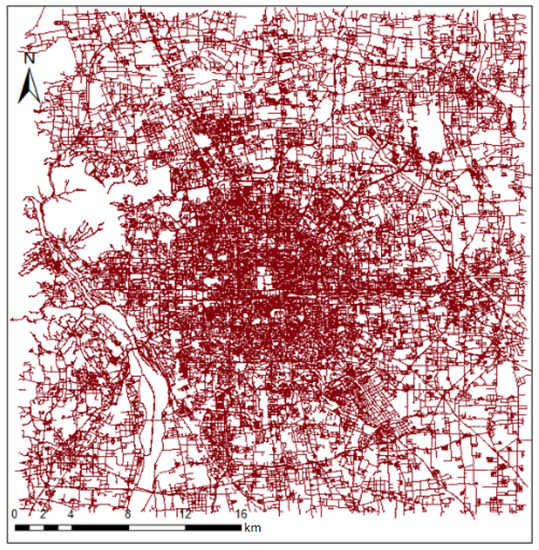
Figure 5. Beijing road network.

A GPS trajectory of this dataset is defined as a series of time-stamped points, each containing the parameters information, including latitude, longitude, and altitude. This total dataset consists of approximately 17,000 different transportation mode trajectories for an average period of 50,000 h, from which more than 30,000 trajectory transportation modes are car and taxi. Various GPS loggers and phones registered these trajectories and have a range of sampling speeds. In this dataset, 91.5% of the trajectories are recorded in a dense representation, for example, every one to five seconds or five to ten meters per point. This dataset listed a wide range of outdoor activities of people. In other study areas, these trajectory datasets are used, which show stability, correctness, and coherence, such as accessibility pattern extraction, consumer behavior identification, location-based social media platforms, information safety, and different position suggestions.

6.2. Trajectory Data Preprocessing

6.2.1. Map Matching

Due to GPS positioning and digital road network flaws, taxi GPS observations may not exactly lay on road network connections, and a taxi may have traveled over many network links. A cab may have passed over many network connections during subsequent observations due to the very low sample level. Hence, by accurately tracking GPS observations on the road network and reconstructing trajectory paths, a dynamic programming map-matching (MDP-MM) multicriteria approach is utilized to overcome this issue [35]. Using [35], this is built to enhance the technique of determining the missing road network links. In this way, we avoid improperly initializing the tag/ label in the path-finding process. The second strategy is establishing the candidate route by a single path-finding procedure at a candidate location rather than continuously searching the shortest routes from preceding candidate locations, as achieved in the standard Dijkstra algorithm.

6.2.2. Trajectory Segmentation

For a different method to find the similarity, trajectory segmentation splits a trajectory into chunks/fragments by time interval. Two trajectory points with considerable time intervals cannot be converted into CLR, and two discontinuous points will cause an error in the result. The two trajectory points with short time intervals are on a road segment, and the middle trajectory point can be interpolated by linear interpolation. If the time interval is large, there will be significant errors in interpolation, especially if the two points are on different roads. When the interval between the two trajectory points is more than 300 s, the trajectory points are not sampled continuously, because using this trajectory for linear interpolation is inaccurate. When the time interval between two trajectory points is less than 0.0000001, the sampling time of these two trajectories is too close, so they are redundant points. That is why they are not used for interpolation.

6.2.3. Spatiotemporal Data Model

The CLR approach handles shifting object indexes and transforms 3D road network-constrained time geographic entities in $(x,y,t)$ space to $2\mathrm{D}$ entities in CLR space. The geographic point $\left(x_i,y_i\right)$ in the road network is equivalently represented by the linear reference $\left(l_u,m_i\right)$. If $z_i^u=l_u,m_i$ and $m_i\in (0,1)$ are integrated into a single real value. $l_i$ is the link identity, a distinct positive integer number. The $z_i^u$ value may be readily converted to a location using dynamic subdivision and is also identical to $\left(x_i,y_i\right)$ in $2mathrm$. A unique 2D point ${\tilde{c}}_i^u=\left(z_i,t_i\right)$ in $(z,t)$ space, also known as the CLR space, may be used to represent any 3D point $c_i^u=\left(x_i,y_i,t_i\right)=\left(l_u,m_i,t_i\right)$ in the road network.

The spacetime route is altered in CLR space, and ${\tilde{P}}^q$ consists of a number of disconnected LineString polyline components. Each line string set of discontinuous components in the structure $<\cdots ,{\widehat{R}}_u^q,\cdots >$ corresponds to $R_u^q$ in $(x,y,t)$ 3D space, denoting the ongoing movement of a person along a specific connection. Each segment $s_{ij}$ in the set is a straight line in CLR space connecting two consecutive control points, ${\tilde{c}}_i^u=\left(z_i,t_i\right)$ and ${\tilde{c}}_j^u=\left(z_j,t_j\right)$, on the same link.

6.3. Prototype System Development

This research prototype is divided into two main parts: LCSS similarity and clustering. We use the LCSS approaches to find similarity distance measured in two different ways. One way is using the buffering technique, and the other is without the buffer. Before creating the buffer, we convert the spacetime path (trajectory 3D) into CLR space, which is 2D, so we generate the buffer over CLR and then apply LCSS on buffer-generated CLR space. We find the similarity measure directly (LCSS without buffer) between two spacetime paths with time and distance thresholds. The time threshold is used to find the similarity on each 20 s and the distance threshold measures the outliers. For the clustering of these similarities, we use two clustering approaches, including hierarchal-based and density-based clustering, which is a more efficient way to present the spacetime trajectory clustering.

The following describes the hardware and software configuration. In order to store, index, and query spacetime pathways (trajectories) in CLR space, we developed ArcSDE 10.2 and SQLServer as the spatial database. The geo-computational algorithm Visual C# is used to create network trajectory buffers along CLR. The ArcEngine 10.2 development kit is used to implement the specified LCSS spacetime operations in Visual C#. Python is used to create hierarchical-based clustering, whereas Visual C# is used to create the density-based clustering method DBSCAN.

7. Experimental Evaluation of Trajectory Data Clustering

Experiment 1: Impact of SP-Analysis on similarity

In this experiment, we calculate the LCSS similarity using two techniques, including LCSS with buffer and LCSS without buffer, with two different length trajectories and with two different numbers of trajectories, as shown in Table 1.

Table 1. Dataset metadata.

Datasets	Number of Trajectory	Average Length	Average Duration
D1	17	40 km	1.2 h
D2	50	150.3 km	4.8 h

Firstly, for LCSS with buffer, we convert the given dataset of trajectories in Compress Liner Reference (CLR). We generate the buffer in road network space alone and the trajectory with a given buffer threshold of 200 m. Moreover, we also observe whether the trajectory lies in the buffer or not. We calculate the time duration of the target trajectory in the buffer. Secondly, we use traditional methods to calculate LCSS. This method uses dynamic programming algorithms to solve LCSS. In solving the LCSS, the matched elements are obtained, and the time duration is represented by the LCSS of the two trajectories obtained from the matched elements in the experiment. Among them, the time threshold $T_1$ and space threshold $T_2$ for judging whether the elements match are 10 s and 200 m, respectively. Table 2 describes the result of LCSS similarity-based time consumption with buffer and without buffer.

Table 2. Time consumption of LCSS similarity calculation.

Dataset	LCSS with Buffer (d = 200 m)			LCSS without Buffer (${\mathit{T}}_1$ = 10 s, ${\mathit{T}}_2$ = 200 m)
	Buffer Create	SP-Analysis	Overall	Overall
D1	14.361 s	19.328 s	33.689 s	9397.32 s
D2	37.424 s	422.584 s	460.008 s	253,049.97 s (=2.93 days)

Based on the previous result, we analyze that when we give the dataset of 17 trajectories, the buffer is created within approximately 14 s and, for 50 trajectories, within 37 s, meaning it takes less than 1 s for each trajectory. Additionally, then, if we find the LCSS similarity, it takes approximately 34 s and the overall time consumption for a total of 17 trajectories whose length is no more than 2 h. For the same dataset, the computation time of LCSS without a buffer is too much compared with finding LCSS with a buffer, even though the dataset is 2 h at maximum. This is because the traditional LCSS method needs to calculate LCSS for each pair of trajectories. In contrast, the SP-Analysis-based method does not need to do so. At the same time, the traditional LCSS method needs to calculate a large number of road network distances, which can be avoided in the SP-Analysis-based method. The same point shows in the dataset of 50 trajectories; we observe that the time consumption of 460.008 s with buffer is much less than the time consumption of 253,049.97 s without buffer. This is why we use the buffering technique to speed up LCSS similarity analysis.

Experiment 2: Analysis of DBSCAN with Hierarchical Clustering

The parameter’s settings are reasonable and dramatically influence the clustering quality in our work. The input parameters of the DBSCAN clustering method based on LCSS $\epsilon$ and $MinClrs$ were determined in the experiment according to the method provided by the author of the original DBSCAN algorithm. First, $MinClrs$ is determined according to $k=In\left|D\right|$, where D represents the trajectory dataset and $k=MinClrs$. Second, calculate the LCSS of each trajectory to its k-th nearest trajectory. When sorting the trajectories in descending order of the k-th nearest similarity value, the sorted k-th similarity graph will give us some directions about the density distribution in the database. As shown in Figure 6, select the k-th similarity value corresponding to the first trajectory in the first “valley” (red line in the graph) of the sorted k-th similarity graph as the input parameter $\epsilon$. The trajectory dataset D2 is used for analysis in Figure 6, where the k value is set to 4.

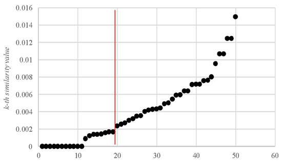
Figure 6. Sorted k-th similarity graph of D2 dataset.

After visual analysis of the sorted k-th similarity graph, the input parameter $\epsilon$ of the trajectory Dataset 1 is set to 0; the input parameter $MinClrs$ of the trajectory Dataset 1 is set to 2. Furthermore, the $\epsilon$ of the trajectory Dataset 2 is set to 0.002; the $MinClrs$ of the trajectory Dataset 2 is set to 4.

Whether the parameter configuration becomes suitable or not has a significant impact on the accuracy of the clustering result. There are three input parameters of the hierarchical clustering method based on LCSS: the spatial threshold $\delta$, linkage type (ward, maximum or complete, and average and single), and similarity matrix. The similarity between two trajectories between two points is calculated by LCSS using the buffer and with the buffering technique along the road network space.

The main work during hierarchical clustering of linkage types is determining linkage type. We use the ward linkage type, in which the algorithm updates the distance matrix at every iteration to represent the distance of the newly formed cluster.

Figure 7 represents the hierarchical clustering of the 50 trajectories dataset by the dendrogram. On the x-axis, the trajectory label is displayed, which combines with another trajectory on each level. A similarity value between trajectories is displayed on the y-axis of the dendrogram. Each level of the trajectory cluster depends on the similarity value, which we calculate by LCSS and store in the distance matrix.

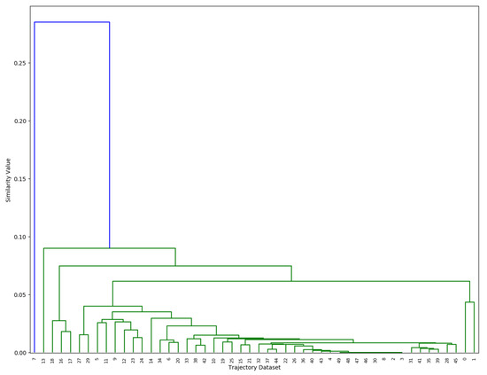
Figure 7. Hierarchical clustering dendrogram of 50 trajectories. Blue dendrogram is the longest trajectory in our work.

Table 3 shows the time consumption of clustering with LCSS similarity measure. Total time consumption over creating clustering with computing the LCSS of the 17 trajectories dataset and then DBSCAN and hierarchical clustering equals 33.690 s. For the over 50 trajectories dataset with more than 4 h, the time consumption to find the LCSS with buffer and then clustering is almost the same, which is approximately 460 s. We also show the comparison of our work with Chen et al. [34] and Yuan et al. [16], and it can be seen that our method takes less time when combined with DBSCAN and HCA.

Table 3. Time consumption of clustering.

Number of Trajectory	LCSS + DBSCAN	LCSS + HCA	Chen et al. [34]	Yuan et al. [16]
17	33.690 s	33.690 s	36.330 s	39.253 s
50	460.009 s	460.010 s	471.52 s	480.32 s

Visual Analysis of Trajectory Clustering

Here, we present a visualization of the results of trajectory clustering in 3D $(x,y,t)$ space. The x-axis represents the latitude, the y-axis represents the longitude, and the z-axis represents the time. This 3D visualization of the clustering result is based on Figure 7. The hierarchical clustering dendrogram of 50 trajectories at the y-axis shows the similarity values. These three clusterings create 0.078 similarity values that contain different numbers of trajectories in the cluster. These 3D representations are shown in the dendrogram (See Figure 7).

Figure 8 shows cluster 1 of trajectory D1, which contains the set of 50 trajectories with an average length of 150.3 km and an average duration of 4 h. This cluster is based on the value of similarity we find using the LCSS. Figure 9 shows the cluster of remaining trajectories from the D2 of 44 trajectories with different lengths, and Figure 10 and Figure 11 show the single trajectory. Distinct colors represent unique trajectories from the data in Figure 8, Figure 9, Figure 10 and Figure 11.

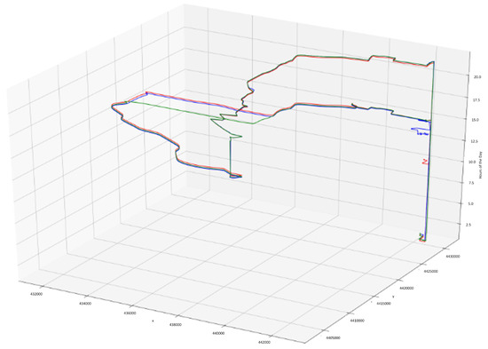
Figure 8. 1st Cluster with 4 trajectories.

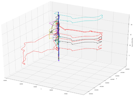
Figure 9. 2nd Cluster with 44 trajectories.

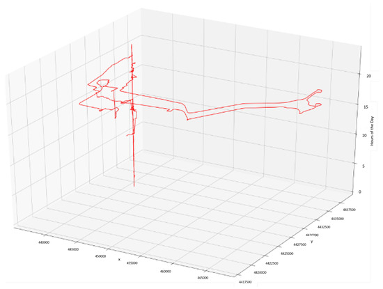
Figure 10. 3rd Cluster with single trajectory.

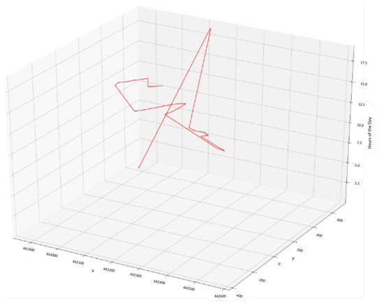
Figure 11. 4th Cluster with single trajectory.

8. Conclusions

This study proposes an efficient density-based clustering method for network constraint trajectories using Beijing’s GeoLife Project dataset. The approach enhances the spatiotemporal cluster by using the buffering technique and CLR space, and we find valid trajectories from raw input data using map matching to locate missing points. We use minimum and maximum thresholds for segmentation, with interpolation providing more accuracy after these thresholds. Our spatiotemporal data model transforms the road network space into CLR space, and we create a buffer along CLR, finding the similarity between trajectories within the buffer using the LCSS similarity metric. We apply different clustering techniques, including DBSCAN and hierarchical clustering, based on LCSS similarity, and the results show a significant reduction in time consumption using the buffering technique.

Our proposed method has potential applications in transportation planning and smart vehicle mobility, helping optimize traffic on roads and improving infrastructure in smart planning. Future work could improve clustering efficiency by exploring different similarity techniques or using F-heap data structures, indexing techniques, or non-SQL databases to reduce computation costs. Overall, this study offers a promising approach for clustering trajectory data with network constraints, paving the way for further research in this field.

References

- Daepp, M.I.; Binet, A.; Gavin, V.; Arcaya, M.C.; Consortium, H.N.R. The moving mapper: Participatory action research with big data. J. Am. Plan. Assoc. 2022, 88, 179–191. [Google Scholar] [CrossRef]
- Quy, V.K.; Nam, V.H.; Linh, D.M.; Ban, N.T.; Han, N.D. Communication solutions for vehicle ad-hoc network in smart cities environment: A comprehensive survey. Wirel. Pers. Commun. 2022, 122, 2791–2815. [Google Scholar] [CrossRef]
- Iliashenko, O.; Iliashenko, V.; Lukyanchenko, E. Big data in transport modelling and planning. Transp. Res. Procedia 2021, 54, 900–908. [Google Scholar] [CrossRef]
- Shu, W.; Li, Y. A novel demand-responsive customized bus based on improved ant colony optimization and clustering algorithms. IEEE Trans. Intell. Transp. Syst. 2022. [Google Scholar] [CrossRef]
- Hamdi, A.; Shaban, K.; Erradi, A.; Mohamed, A.; Rumi, S.K.; Salim, F.D. Spatiotemporal data mining: A survey on challenges and open problems. Artif. Intell. Rev. 2022, 55, 1441–1488. [Google Scholar] [CrossRef] [PubMed]
- Yu, W.; Huang, Q. A deep encoder-decoder network for anomaly detection in driving trajectory behavior under spatio-temporal context. Int. J. Appl. Earth Obs. Geoinf. 2022, 115, 103115. [Google Scholar] [CrossRef]
- Toch, E.; Lerner, B.; Ben-Zion, E.; Ben-Gal, I. Analyzing large-scale human mobility data: A survey of machine learning methods and applications. Knowl. Inf. Syst. 2019, 58, 501–523. [Google Scholar] [CrossRef]
- Reyes, G.; Lanzarini, L.; Hasperué, W.; Bariviera, A.F. Proposal for a pivot-based vehicle trajectory clustering method. Transp. Res. Rec. 2022, 2676, 281–295. [Google Scholar] [CrossRef]
- Paterson, M.; Dančík, V. Longest common subsequences. In Proceedings of the International Symposium on Mathematical Foundations of Computer Science; Springer: Berlin/Heidelberg, Germany, 1994; pp. 127–142. [Google Scholar]
- Nakamura, T.; Taki, K.; Nomiya, H.; Seki, K.; Uehara, K. A shape-based similarity measure for time series data with ensemble learning. Pattern Anal. Appl. 2013, 16, 535–548. [Google Scholar] [CrossRef]
- Briggs, I.C. Machine contouring using minimum curvature. Geophysics 1974, 39, 39–48. [Google Scholar] [CrossRef]
- Hoerl, A.E.; Kennard, R.W. Ridge regression: Biased estimation for nonorthogonal problems. Technometrics 1970, 12, 55–67. [Google Scholar] [CrossRef]
- Wolny, A.; Ogryzek, M.; Źróbek, R. Challenges, opportunities and barriers to sustainable transport development in functional urban areas. In Environmental Engineering. Proceedings of the International Conference on Environmental Engineering; ICEE Vilnius Gediminas Technical University, Department of Construction Economics: Vilnius, Lithuania, 2017; Volume 10, pp. 1–9. [Google Scholar]
- Besse, P.C.; Guillouet, B.; Loubes, J.M.; Royer, F. Review and perspective for distance-based clustering of vehicle trajectories. IEEE Trans. Intell. Transp. Syst. 2016, 17, 3306–3317. [Google Scholar] [CrossRef]
- Zheng, S.; Guan, D.; Yuan, W. Semantic-aware heterogeneous information network embedding with incompatible meta-paths. World Wide Web 2022, 25, 1–21. [Google Scholar] [CrossRef]
- Yuan, H.; Chen, B.Y.; Li, Q.; Shaw, S.L.; Lam, W.H. Toward spacetime buffering for spatiotemporal proximity analysis of movement data. Int. J. Geogr. Inf. Sci. 2018, 32, 1211–1246. [Google Scholar] [CrossRef]
- Yuan, G.; Sun, P.; Zhao, J.; Li, D.; Wang, C. A review of moving object trajectory clustering algorithms. Artif. Intell. Rev. 2017, 47, 123–144. [Google Scholar] [CrossRef]
- Han, J.; Kamber, M.; Pei, J. Data Mining: Concepts and Techniques, 3rd ed.; Morgan Kaufmann: Waltham, MA, USA, 2011. [Google Scholar]
- Ding, C.H.; He, X.; Zha, H.; Gu, M.; Simon, H.D. A min-max cut algorithm for graph partitioning and data clustering. In Proceedings of the 2001 IEEE International Conference on Data Mining, San Jose, CA, USA, 29 November–2 December 2001; pp. 107–114. [Google Scholar]
- Li, H.; Liu, J.; Wu, K.; Yang, Z.; Liu, R.W.; Xiong, N. Spatio-Temporal Vessel Trajectory Clustering Based on Data Mapping and Density. IEEE Access 2018, 6, 58939–58954. [Google Scholar] [CrossRef]
- Cong, J.; Smith, M. A parallel bottom-up clustering algorithm with applications to circuit partitioning in VLSI design. In Proceedings of the 30th International Design Automation Conference, Dallas, TX, USA, 14–18 June 1993; pp. 755–760. [Google Scholar]
- Böhringer, C.; Rutherford, T.F. Integrated assessment of energy policies: Decomposing top-down and bottom-up. J. Econ. Dyn. Control 2009, 33, 1648–1661. [Google Scholar] [CrossRef]
- Guha, S.; Rastogi, R.; Shim, K. Cure: An efficient clustering algorithm for large databases. Inf. Syst. 2001, 26, 35–58. [Google Scholar] [CrossRef]
- Birant, D.; Kut, A. ST-DBSCAN: An algorithm for clustering spatial–temporal data. Data Knowl. Eng. 2007, 60, 208–221. [Google Scholar] [CrossRef]
- Parikh, M.; Varma, T. Survey on different grid based clustering algorithms. Int. J. Adv. Res. Comput. Sci. Manag. Stud. 2014, 2, 427–430. [Google Scholar]
- Bouveyron, C.; Brunet-Saumard, C. Model-based clustering of high-dimensional data: A review. Comput. Stat. Data Anal. 2014, 71, 52–78. [Google Scholar] [CrossRef]
- Zhang, Z.; Huang, K.; Tan, T. Comparison of similarity measures for trajectory clustering in outdoor surveillance scenes. In Proceedings of the 18th International Conference on Pattern Recognition (ICPR’06), Hong Kong, China, 20–24 August 2006; Volume 3, pp. 1135–1138. [Google Scholar]
- Chen, L.; Özsu, M.T.; Oria, V. Robust and fast similarity search for moving object trajectories. In Proceedings of the 2005 ACM SIGMOD International Conference on Management of Data, Baltimore, MD, USA, 14–16 June 2005; pp. 491–502. [Google Scholar]
- Eiter, T.; Mannila, H. Computing Discrete Fréchet Distance 1994. Available online: https://www.researchgate.net/publication/228723178_Computing_Discrete_Frechet_Distance (accessed on 2 December 2022).
- Chen, J.; Wang, R.; Liu, L.; Song, J. Clustering of trajectories based on Hausdorff distance. In Proceedings of the IEEE 2011 International Conference on Electronics, Communications and Control (ICECC), Ningbo, China, 9–11 September 2011; pp. 1940–1944. [Google Scholar]
- Rick, C. Efficient computation of all longest common subsequences. In Proceedings of the Scandinavian Workshop on Algorithm Theory, Bergen, Norway, 5–7 July 2000; Springer: Berlin/Heidelberg, Germany, 2000; pp. 407–418. [Google Scholar]
- Vlachos, M.; Kollios, G.; Gunopulos, D. Discovering similar multidimensional trajectories. In Proceedings of the IEEE 18th International Conference on Data Engineering, San Jose, CA, USA, 26 February–1 March 2002; pp. 673–684. [Google Scholar]
- Chen, B.Y.; Yuan, H.; Li, Q.; Shaw, S.L.; Lam, W.H.; Chen, X. Spatiotemporal data model for network time geographic analysis in the era of big data. Int. J. Geogr. Inf. Sci. 2016, 30, 1041–1071. [Google Scholar] [CrossRef]
- Chen, B.Y.; Luo, Y.B.; Jia, T.; Chen, H.P.; Chen, X.Y.; Gong, J.; Li, Q. A spatiotemporal data model and an index structure for computational time geography. Int. J. Geogr. Inf. Sci. 2023, 37, 550–583. [Google Scholar] [CrossRef]
- Chen, B.Y.; Yuan, H.; Li, Q.; Lam, W.H.; Shaw, S.L.; Yan, K. Map-matching algorithm for large-scale low-frequency floating car data. Int. J. Geogr. Inf. Sci. 2014, 28, 22–38. [Google Scholar] [CrossRef]
Disclaimer/Publisher’s Note: The statements, opinions and data contained in all publications are solely those of the individual author(s) and contributor(s) and not of MDPI and/or the editor(s). MDPI and/or the editor(s) disclaim responsibility for any injury to people or property resulting from any ideas, methods, instructions or products referred to in the content. |
© 2023 by the authors. Licensee MDPI, Basel, Switzerland. This article is an open access article distributed under the terms and conditions of the Creative Commons Attribution (CC BY) license (https://creativecommons.org/licenses/by/4.0/).