A Self-Attention Model for Next Location Prediction Based on Semantic Mining

Abstract

With the rise in the Internet of Things (IOT), mobile devices and Location-Based Social Network (LBSN), abundant trajectory data have made research on location prediction more popular. The check-in data shared through LBSN hide information related to life patterns, and obtaining this information is helpful for location prediction. However, the trajectory data recorded by mobile devices are different from check-in data that have semantic information. In order to obtain the user’s semantic, relevant studies match the stay point to the nearest Point of Interest (POI), but location error may lead to wrong semantic matching. Therefore, we propose a Self-Attention model for next location prediction based on semantic mining to predict the next location. When calculating the semantic feature of a stay point, the first step is to search for the k-nearest POI, and then use the reciprocal of the distance from the stay point to the k-nearest POI and the number of categories as weights. Finally, we use the probability to express the semantic without losing other important semantic information. Furthermore, this research, combined with sequential pattern mining, can result in richer semantic features. In order to better perceive the trajectory, temporal features learn the periodicity of time series by the sine function. In terms of location features, we build a directed weighted graph and regard the frequency of users visiting locations as the weight, so the location features are rich in contextual information. We then adopt the Self-Attention model to capture long-term dependencies in long trajectory sequences. Experiments in Geolife show that the semantic matching of this study improved by 45.78% in TOP@1 compared with the closest distance search for POI. Compared with the baseline, the model proposed in this study improved by 2.5% in TOP@1.

1. Introduction

In recent years, with the rise in positioning devices, Internet of Things (IoTs) and smart city concepts, mobile phone positioning data and social network data have provided a large number of continuous location trajectory data; research on trajectory prediction and analysis has become increasingly popular, and related research topics have gradually received attention. By predicting the location people will visit in the future, advertising companies can immediately provide location-related advertisements [1] and government departments can predict the flow of people for traffic planning in order to ease traffic congestion [2]. Platforms such as Uber are also using next location prediction technology to better estimate customer’s travel needs and allocate resources accordingly [3]. In the past, the most commonly used method for location prediction was either Markov chain [4,5,6] or machine learning [7], but due to the large amount of trajectory data, many related studies have begun using deep learning technology to predict the user’s next location [1,2,8,9,10,11,12,13].

Many relevant studies often consider spatiotemporal features such as location features and temporal features when using deep learning to predict the user’s next location. However, the check-in data shared through LBSN hide semantic information related to life patterns; if the model considers semantic features, it can obtain more detailed characteristics about the user’s life pattern and location preference. Therefore, semantic features can help enhance the performance of next location prediction. However, not all users like to share their check-in information on LBSN. The trajectory data recorded by mobile devices are not like the check-in data of social networks that have complete semantic annotation information. In order to understand the user’s semantic trajectory behavior, relevant studies [1,14] matched the trajectory stay point to the nearest Point of Interest (POI). However, location error may lead to incorrect semantic matching; incorrect semantic matching causes the model to learn wrong semantic behavior patterns.

Due to the motivation mentioned above, we propose a Self-Attention model for next location prediction based on semantic mining. In our model, we have location features, temporal features, semantic features and user features, while focusing on how to extract semantic features. For semantic features, the stay points of trajectory are matched to the k-nearest POI. We then use the reciprocal of the distance from the stay points to the k-nearest POI and the number of categories as weights. Finally, we use probability to express semantic features without losing other important semantic information. This method solves the wrong semantic matching problem caused by location error and also considers more of the spatial information on POIs. Furthermore, we combine sequential pattern mining to further infer user’s semantic behaviors, which can result in richer semantic features. For temporal features, we adopt Time2vec to learn periodic features from the time features. For location features, we adopt the Node2vec to extract contextual features of the trajectory sequence. Finally, we concatenate the features as the input of the prediction mode and we adopt Self-Attention to capture long-term dependencies in sequences; Self-Attention uses fully connected layers to consider the information of each stage together, so it retains more long-term information. In the output of Self-Attention, we consider the user ID feature to make the model more personal and obtain prediction results. As a result, we can predict the user’s future location by inputting the user’s past locations, timestamps and semantics into Self-Attention.

The contributions of this paper are listed below:

• We design semantic matching to effectively extract the semantic feature of each stay point. We then combine sematic matching with sequential pattern mining to result in richer semantic features.
• We use Node2vec and Time2vec, which consider the interaction of each location and the periodicity of the time series.
• We adopt Self-Attention to predict the user’s next trajectory for solving the problem with RNN (Recurrent Neural Network); the problem with RNN is that long-term memory is diminished with each transfer.
• We use Geolife dataset for our experiments. Based on experiment results, our method is better than a number of state-of-the-art methods.

The following is the structure of this paper. First, we review relevant research on location prediction in Section 2. Next, Section 3 is the problem statement, explaining the numerous terms in location prediction. Then, Section 4 explains the method we proposed for location prediction. Following that, we evaluate our model’s performance and compare its accuracy to that of other models in Section 5. In Section 6, we conclude our findings and briefly discuss future works.

2. Related Work

In this section, we discussed important literature regarding location prediction. In terms of location prediction, besides the design of the model itself, there are many different methods for feature extraction, such as temporal, location and semantics. Therefore, we can separate the literature into two topics: location prediction and feature extraction.

2.1. Location Prediction

In the first part, we introduce the literature on location prediction. In 2018, Xia et al. considered both stay points and semantic information and used a decision tree for location prediction [7]. A Markov chain is often used to deal with location predictions. A Markov chain is a method with discrete random variables that capture the regularity of human movement. In 2018, Jiang et al. extended the first-order Markov chain to the k-order Markov chain to consider more important historical information [5]. In 2018, Xia et al. established a variable-order Markov chain to predict location based on the matching of the historical trajectory and the current trajectory [6]. In 2017, Fernandes et al. combined Naïve Bayesian Classification algorithm and the Markov model to predict next location [4]. However, the Markov chain transfer process is memoryless, which means that the result of the current state is only influenced by the previous state.

Recently, many studies have used deep learning to predict the user’s future location. RNN is a typical deep learning model for time series. Since it can transfer long-term memory to the previous state, it solves the Markov chain problem (the Markov chain is limited to the previous state). The SERM model proposed by Yao et al. learns embeddings for multiple features (user, location, time, semantic) and uses Long Short-Term Memory (LSTM) to forecast the next location [12]. In 2020, Su et al. considered both propagation directions of LSTM; they used Bi-directional Long Short-Term Memory (BiLSTM) to predict the user’s next location [9]. Furthermore, in 2020, Xu et al. combined BiLSTM with the Similarity-based Markov Model (SMM) to predict the user’s next location [1]. The problem with RNN is that long-term memory is diminished with each transfer. The Attention mechanism [10] improves this because the Attention mechanism does not pass the long-term memory through each stage. In other words, the Attention mechanism uses a fully connected layer to consider the information of each stage together, so it retains more long-term memory. In 2018, Al-Molegi et al. adopted the Attention mechanism in their neural network to capture long-term dependencies in trajectory sequences to predict the user’s future location [8]. In 2020, Zhang et al. designed a variant of LSTM with an Attention mechanism to better capture spatiotemporal dependencies [13]. Wang et al. designed a variant of the Attention mechanism; this variant focuses on the time interval and distance interval, thus enriching the continuity of spatiotemporal, which can better distinguish each location [11]. However, in 2020, Feng et al. proposed a unique Attention mechanism application. This method uses the user’s current trajectory with LSTM to predict the user’s future location, but also combines the historical trajectory with Attention to capture multi-level periodicity. In addition to considering location feature, time feature, semantics feature and user ID feature, they also consider user text feature [2]. In 2021, Wen et al. adopted LSTM to capture long-term and short-term spatiotemporal dependencies, and Attention mechanism is introduced to distinguish each location in different contexts [3]. In addition to the structure of the neural network, the feature extraction is also a key point that affects the next location prediction.

2.2. Feature Extraction

In the second section, we introduce feature extraction methods. Trajectories have three main features: location, time and semantic. The location feature is usually a one-hot vector whose dimension is determined by the number of locations. Due to the large number of locations, the curse of dimensionality occurs when training the model. In order to avoid this problem, relevant studies use embedding layer (full connection), which reduces a high-dimensional one-hot vector to a low-dimensional space, which eliminates the curse of dimensionality in the prediction model [5,12,13]. On the other hand, since trajectories have contextual features like words, some studies use Word2vec [15] to extract location features [1,11]. The principle of Word2vec is to use the weights of the fully connected layer of a classifier as word vectors. In this classifier, the word’s one-hot vectors are input, then fed into a fully connected layer, and then fed to a SoftMax to obtain the probability of the contexts. Finally, the weight of the fully connected layer after training will be obtained, which is the word vectors of Word2vec. The difference between the embedding layer and Word2vec is explained as follows. Word2vec is an unsupervised learning method that uses context to learn word embedding; it is a pretrained model. In the embedding layer, the weight of a full connection is updated based on the label information learning. In order to achieve a higher supervised learning effect, the embedding layer is used as a layer of the network to learn and adjust according to the target. But, Word2vec and full connection omit a lot of valid contexts, which makes it difficult to contain more spatial information and distinguish between each location. Therefore, in the loc2vec embedding method proposed by Sassi et al., each location is encoded as a vector, whereby the more often two locations co-occur in the trajectory sequences, the closer their vectors will be [16]. Furthermore, the graph-embedding method of Node2vec is based on Word2vec; its directed weighted graph carries more spatiotemporal context information [17]. In 2021, Wen et al. used Node2Vec to extract location feature, which encodes each location in all trajectories to construct a directed weighted graph. It then takes the number of visits to the location as the weight of the graph, which reflects the visit order preference and frequency [3]. Also inspired by Word2vec, in 2019, Xu et al. proposed an embedding model called Venue2Vec, which combines spatiotemporal context, semantic information and sequence relationships; semantics of the same type and locations that are close or that users frequently visit will have similar vector spaces [18]. In addition to Word2vec-based methods, in 2020, Chen et al. proposed the Convolutional Embedding Model (CEM), which embeds the locations by using convolutions [19].

In terms of temporal features, some studies usually perform a series of preprocessing in timestamp to extract temporal features for the next location prediction, such as converting timestamps into hours, days, weeks, months and seasons. However, temporal features are cyclical. Taking hours as an example, temporal features are usually represented by 1 to 24, although using hours to represent the temporal features can reflect the periodicity, it may not be able to fully express the period of time. Therefore, Lu et al. considered the cyclic features of time, and designed the coordinates on a unit circle using the sine and cosine functions to represent the cyclic features of time [20]. Kazemi et al. proposed Time2vec. This method uses temporal features to learn the phase-shift and frequency of the sine function; it can learn periodic temporal features, which allows the neural network to better learn temporal features [21].

In terms of semantic feature extraction, trajectory data are divided into check-in data and GPS trajectory data. Check-in data such as Gowalla dataset and Foursquare dataset, usually have semantic information. On the other hand, GPS trajectory data such as the Geolife dataset do not record semantic information. First, we introduce the semantic feature extraction of check-in data. In 2016, Xie et al. used graph structure to embed semantic features to encode users’ semantic trajectory in a vector space [22]. In 2019, Cao et al. proposed habit2vec, which keeps the original user’s pattern of living habits [23]. In 2020, Zhang et al. proposed Sen2vec, which calculates semantic vectors according to the frequency and principal component analysis [13]. As for GPS trajectory data, in order to extract semantic information, it is necessary to collect POI data and match the stay points. If the POI is not considered, the semantic information can be extracted from the trajectory sequence data alone. In 2009, Ye et al. used the sequential pattern mining to infer users’ semantic behavior [24]. In 2016, Chen et al. proposed semantic trajectory patterns, which are moving patterns with location, time and semantic attributes. Given a user’s trajectory, their objective is to mine common semantic trajectory patterns [25].

3. Problem Statement

We explicitly define the notations used in the location prediction issue in this section. Our topic is to predict a user’s future location based on their trajectory. The notations concerning location prediction are listed in Table 1.

Table 1. The notations about location prediction.

Notation	Description
$tra, p$	Trajectory, GPS point
$u, U$	User, set of users
$s, S$	Stay point, set of stay points
$lat, lng$	Latitude, longitude
$t_e,t_l$	Time of entering and leaving a stay point
$poi,POI$	POI, set of POIs
$ty, TY$	A type of POI, set of types
$\varsigma$	Semantics
$l, L$	Stay grid, set of stay grids

Definition 1.

Trajectory: A time-ordered sequence of GPS points, a GPS trajectory $tra=\{p_1,p_2,\dots p_n\}$, each GPS point $p_i$ is a 4-tuple $p_i=(u,p.{lat}_i,{p.lng}_i,{p.t}_i)$, where the user ID, latitude, longitude and time are denoted by $u$, $p.lat$, $p.lng$ and $p.t$, respectively.

Definition 2.

Stay point: Given a set of sequential GPS points $tra=<p_x,\dots ,p_i,\dots ,p_y>$ satisfying, $\left(1\right).\forall x\le i\le y$, $\left(2\right).Distance\left(p_x,p_i\right)\le {\theta }_d$, $\left(3\right).Distance(p_x,p_{y+1})>{\theta }_d$, and $(4).TimeDifference(p_y,p_x)>{\theta }_t$. $S=\{s_1,s_2,\dots ,s_n\}$, a stay point is a 5-tuple $s=(u,s.lat,s.lng,t_e,t_l)$, where $s.lat$ and $s.lng$ denote the average latitude and longitude of GPS point, respectively, and are defined as (1), where $t_e$ and $t_l$ refer to the time of entering and leaving a stay point, respectively.

$$s.lat=\frac{{\sum }_{i=x}^y{p}_i.lat}{\left|P\right|}, s.lng=\frac{{\sum }_{i=x}^y{p}_i.lng}{\left|P\right|}$$

(1)

Definition 3.

POI: POI (Point of Interest) $poi$ refers to a landmark on the electronic map, which can be a restaurant, a bank, a school, a hospital, etc., $poi\in POI$ , which is composed of the type of poi $ty\in TY$, the latitude $poi.lat$ and the longitude $poi.lon$.

Definition 4.

Semantic: The semantic $\varsigma$ is defined as the purpose of the user visiting a stay point $s$. The semantic $\varsigma$ is calculated by matching the stay point to the k-nearest POI. The dimension of $\varsigma$ is the number of $TY$; each dimension corresponds to a different $poi.ty$. Given a set of consecutive stay points $S=s_1,s_2,\dots ,s_n$, each S will search for k-nearest POI as semantic $\varsigma$.

Definition 5.

Stay grid: We use grids to represent the stay points $L=<l_1,l_2,\dots ,l_n>$, $l=(u,g,t,\varsigma )$, where $g$ is the index of the gird, and we use time of entering stay point $t_e$ as the time of stay grid $t$.

Definition 6.

Trajectory Sequence: According to time window $t_w$, a user’s stay grid sequence $L$ is divided into several subsequences $L=\left\{L_{t_{w_1}},L_{t_{w_2}},\dots ,L_{t_{w_m}}\right\}$, where m is the index of the subsequence. Each$L_{t_w}$ contains several stay grids of $L$ in the time window $t_w$, $i.e., L_{t_w}=\left\{ l_i,l_{i+1},\dots , l_{i+k}\right\},$ if $i<j\le i+k$, then $t_j$ belongs to $t_w$ (the time window $t_w$ can be 1 day, 1 week, 1 month or 1 year). We then convert $L_{t_w}$ into a trajectory sequence using sliding window. Given a subsequence $L_{t_w}=\left\{l_i,l_{i+1},\dots ,l_{i+k}\right\}$, we use sliding window to obtain $L_{SW}=\left\{L_{{sw}_j},L_{{sw}_{j+1}},\dots ,L_{{sw}_{j+k-h}}\right\}$, $L_{{sw}_j}\left\{l_i,l_{i+1},\dots ,l_{i+h-1}\right\}$, where $h$ is the length of the sliding window, whereas $L_{sw}$ is defined as a trajectory sequence.

Definition 7.

Problem: For a user $u \in U$, given a trajectory sequence $L_{sw}=$ $\{l_i,l_{i+1},\dots ,l_{i+h-1}\}$, our purpose is to predict the next location $g_{i+h}$.

4. Proposed Method

In this section, we introduce our proposed method, which is split into three parts. Frist, we introduce the entire model architecture and explain the input and output of the model. Then, we will introduce how we extract input features. Finally, we explain our proposed model in detail.

4.1. System Framework

Our framework is shown in Figure 1. The architecture is divided into three parts: input features (green), prediction model (blue) and predicted results (red). In the beginning, the required data (trajectory data and POI data) are processed to obtain four features: 1. user feature; 2. location feature; 3. temporal feature; 4. semantic feature. Then, we divided the data into training and testing sets. Next, the neural network model is fed the training data (the structure of our model will be discussed at the end of this section). The trained model will generate the anticipated future locations when we feed it the testing data after the training operation.

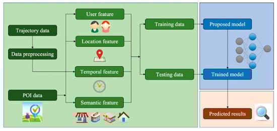
Figure 1. The framework of our research. Source: Icon made by Smashicons, Freepik and dDara from www.flaticon.com (accessed on 31 July 2022).

4.2. Input Features

We have four major features: user feature, location feature, temporal feature and semantic feature. The first three features are obtained from trajectory data, whereas the last feature (semantic feature) is obtained by matching the stay point to the $k$-nearest POI. Therefore, we need two types of data: trajectory data and POI data.

• Trajectory data: The main data for predicting the user’s next location. The location is recorded every 1 to 5 s. Trajectory data record the living habits of users and provide clues for predicting the user’s next location.
• POI data: The POI data in the study area; each poi ∈ POI contains poi.ty, poi.lat and poi.lng.

We will describe how to extract features from data and how to transform data into features in the sections that follow, as well as the methods utilized to achieve important features. These features will be input into the model.

• User Feature: User feature is the user ID $u\in U$. To personalize the prediction model, we consider the user feature $u$($u$ is a one-hot vector whose dimension is the number of users $U$).
• Location Feature: We use stay grid $g$ to represent a location. Stay grid $g$ is one-hot vector, and the dimension of $g$ is determined by the number of grids that cover the study area which users have visited.
• Temporal Feature: Temporal feature reveals what time the information is in. Several methods usually perform a series of preprocessing on timestamps to extract temporal features for the next location prediction, such as converting timestamps into hour, day, week, month and season. In this paper, we convert timestamps into hours (1 to 24) to obtain temporal features t.
• Semantic Feature: Semantic feature $\varsigma$ is defined as the purpose of a user visiting a stay point. Some studies usually match a stay point to the nearest POI. In this paper, we introduce a semantic matching to extract semantic features; the architecture of semantic matching is shown in Figure 2.
  

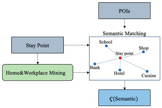  Figure 2. The framework of semantic matching.

When we calculate the semantic vector of the stay point, we consider the $k$-nearest POI. In addition, inspired by Ye et al. [24], we combine sequential pattern mining to mine the user’s home and workplace. We then calculate the semantic vector $\varsigma$ while considering the home and workplace.

We use the stay points $S=\{s_1,s_2,\dots ,s_n\}$ to mine the user’s home and workplace. However, this sequence still cannot be directly applied to mining home and workplace, because no two stay points have the same latitudes and longitudes. For example, stay points at a workplace have different coordinates even though they are very close to each other [24]. To solve this problem, we apply the OPTIC clustering algorithm to find out where the stay points are clustered as demonstrated in Figure 3. The stay points of a user $S=\{s_1,s_2,\dots ,s_n\}$ are collected into a dataset and clustered into several geographic areas $C=\{c_1,c_2,\dots ,c_n\}$. There are two parameters: number of points and distance threshold; we set the number of points at 2 and distance threshold at 45 m. Accordingly, additional stay points will be added to the cluster if there are at least two within 45 m of a clustered stay point. Then, the clustering stay points $C=\{c_1,c_2,\dots ,c_n\}$ will be the input to home and workplace mining.

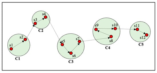
Figure 3. Clustering stay points, where s1–s12 are stay points and C1–C5 are clusters.

Next, we adopt the Closet+ algorithm to mine the home and workplace in the clustering stay points. Figure 4 illustrates an example of home and workplace mining. The first table in Figure 4 means that on day 1, the user went to $c_1,c_3,c_4$; on day 2, the user went to $c_2,c_3,c_5$, and so on. We then count the number of clusters in the database to obtain the second table. Next, we delete the clusters below the min support = 1 in the second table to produce the fourth table. Using the fourth table, we can find the most frequent clusters during the day and night, which we can use to mine the workplace and home clusters. In this paper, we only calculated the first stage of the Closet+ algorithm.

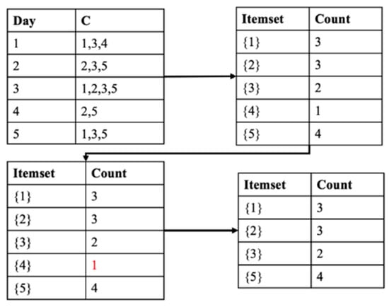
Figure 4. Home and workplace mining.

Next, we will introduce the semantic matching algorithm. The flow chart of the semantic matching algorithm is shown in Figure 5, where $R\in TY$ is real estate, $\varsigma$ is semantic vector (the dimension of semantic vector is the number of different $poi.ty$, in addition to home and workplace) and ${\varsigma }_{temp}$ is temporary register (the same dimension as $\varsigma$). The following explains how to calculate the semantic vector $\varsigma$ of the stay point $s$:

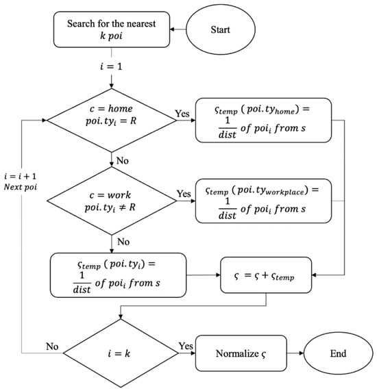
Figure 5. Semantic matching algorithm.

• First, the algorithm searches for the nearest $k$ POI, then starts to calculate the ${\varsigma }_{temp}$ of each $poi$.
• If c = home and $poi.{ty}_i$ = R, then $poi.{ty}_i$ is changed to home. Next, we calculate the reciprocal of the distance between ${poi}_i$ and $s$.
• If c = work and $poi.{ty}_i\ne$ R, then $poi.{ty}_i$ is changed to workplace (because we think that POI that are not R is likely to be workplace). Next, we calculate the reciprocal of the distance between ${poi}_i$ and $s$.
• If $c \ne$ home and c $\ne$ workplace, we directly calculate the reciprocal of the distance between ${poi}_i$ and $s$.
• We repeat $\varsigma =\varsigma +{\varsigma }_{temp}$, and when $i=k$, the loop stops. We then normalize $\varsigma$, ending the algorithm.

We introduce an example of semantic matching in Figure 6. Assuming that there are only three POI types, so the dimension of $\varsigma$ is 5 ([School, Shop, R, Home, Work]), and the k = 4 (the algorithm searches for the nearest four $poi$). The blue dotted lines in Figure 6 are the distance between the stay point $s$ and the four $poi$. Once the algorithm starts, the stay point $s$ will search for the four nearest $poi$. We need to calculate the reciprocal of the distance between the four $poi$ and the stay point, since the clustering stay point $c$ is neither the home cluster nor the workplace cluster. In this example, the semantic feature is calculated as (2).

$$\begin{array}{c}i=1,{\varsigma }_{temp}=\left[\frac{1}{4},0,0,0,0\right],\varsigma =\left[\frac{1}{4},\mathrm{0,0},0,0\right]\\ i=2,{\varsigma }_{temp}=\left[0,\frac{1}{2},0,0,0\right],\varsigma =\left[\frac{1}{4},\frac{1}{2},0,0,0\right]\\ i=3,{\varsigma }_{temp}=\left[0,\frac{1}{3},0,0,0\right],\varsigma =\left[\frac{1}{4},\frac{5}{6},0,0,0\right]\\ i=4,{\varsigma }_{temp}=\left[0,0,\frac{1}{2},0,0\right],\varsigma =\left[\frac{1}{4},\frac{5}{6},\frac{1}{2},0,0\right]\\ \mathrm{N}\mathrm{o}\mathrm{r}\mathrm{m}\mathrm{a}\mathrm{l}\mathrm{i}\mathrm{z}\mathrm{e}\left(\varsigma \right)=[0.157,0.526,0.315,0,0]\end{array}$$

(2)

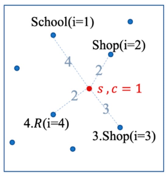
Figure 6. Example of semantic matching.

4.3. Prediction Model

Our prediction model architecture is shown in Figure 7. It uses the features mentioned in input features to obtain the predicted next location. In order to better learn temporal features and location features, we use Time2vec to learn the periodic features of the temporal features and use Node2vec to extract contextual features rich in trajectory sequences. Next, the temporal features, location features and semantic features are concatenated as input for the prediction model. In order to predict the next location, we adopt Self-Attention to solve this issue. Self-Attention is a model that has been successfully used for time-series-forecasting challenges and can model temporal properties well. In order to personalize our model, we add the user ID features to the output of Self-Attention. Finally, we can obtain the final prediction result after SoftMax.

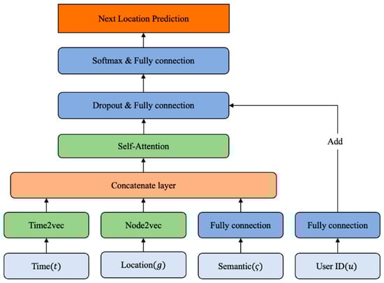
Figure 7. The proposed model.

4.3.1. Temporal Features Extractor

The temporal feature t is a one-dimensional vector represented by hours (1–24). However, time is a periodic feature. Although using hours to represent the temporal features can reflect the periodicity, it may not be able to fully express the period of time. Therefore, inspired by Kazemi et al. [21], we adopt Time2vec to extract the periodic temporal features. The formula of Time2vec is shown as (3), where $\mathbb{t}$ is the dimension of the Time2vec output $B_t^{*}$. The first $b_{t_1}(i=0)$ dimension learns original temporal features, the other dimensions $b_{t_2},\dots ,b_{t_{\mathbb{t}}}(1\le i\le \mathbb{t})$ learn periodic temporal features using the sine function, where ${\omega }_i$ and ${\phi }_i$ are learnable parameters, referring to the phase-shift and frequency of the sine function.

$$\begin{gathered} b_{t_i}=Time2vec\left(t\right)\left[i\right]=\left\{\begin{array}{c}{\omega }_i\tau +{\phi }_i, if i=0\\ \sin \left({\omega }_i\tau -{\phi }_i\right), if 1\le i\le t\end{array}\right. \\ {B}_t^{*}=\left[b_{t_1},b_{t_2},\dots ,b_{t_{\mathbb{t}}}\right], B_t^{*}\in {\mathbb{R}}^{{d_{\mathbb{t}}}_{ }} \end{gathered}$$

(3)

4.3.2. Location Features Extractor

The location feature $g$ is a one-hot vector (the dimension is composed of the number of grids covering the study area). Due to the large number of grids, the dimension of $g$ is extensive, which may lead to the curse of dimensionality, not only increasing the amount of computation, but also making the model easier to overfit. Therefore, we adopt a graph-based embedding method called Node2vec, which encodes each grid in all trajectories to construct a directed weighted graph. It then takes the number of visits to the location as the weight of the graph, which reflects the visit order preference and frequency, while using Breadth-First Search (BFS), Depth-First Search (DFS) and random walks to generate training data. Finally, using Word2vec embeddings to obtain more expressive features that fully consider the interaction between each location and its neighbors, it also can capture richer context spatial information.

In Node2vec, for all the trajectories of all users, we create a directed weighted $Graph=(V,E, W)$, where $V$ is a set of vertices (all grids will be a set of vertices) and $E$ is a set of edges. We define edge $e_{ij}$ as (4):

$$e_{ij}=\left\{\begin{array}{c}1, from{g}_i to g_j\\ 0, unachievable\end{array}\right.{,e}_{ij}\in E$$

(4)

Based on the trajectory movement of all users, we can obtain $E$. The $w_{ij}\in W$ denotes the weight of $e_{ij}$, which is calculated from the total number of visits. Then, Node2vec combines the BFS and DFS to sample the graph. Given the current node $v \in V$, the transition probability of visiting the next node $x$ is shown as (5):

$$P\left(c_i=x\right|c_{i-1}=v)=\left\{\begin{array}{c}\frac{{\pi }_{vx}}{Z}, if\left(v,x\right) ϵ E\\ 0, otherwise\end{array}\right.$$

(5)

Before calculating the transition probability, node $v$ and node $x$ must have an edge link; ${\pi }_{vx}$ is the probability of an unnormalized transition between node $v$ and node $x$, whereas $Z$ refers to the normalization constant. In order to control the random walk strategy, Node2vec uses two hyperparameters (p and q), which is defined as (6):

$$\begin{gathered} {\pi }_{vx}={\alpha }_{pq}\left(\tilde{t},x\right)·w_{vx} \\ {\alpha }_{pq}\left(\tilde{t},x\right)=\left\{\begin{array}{c}\frac{1}{p}, if d_{\tilde{t}x}=0 \\ 1, if d_{\tilde{t}x}=1\\ \frac{1}{q}, if d_{\tilde{t}x}=2\end{array}\right. \end{gathered}$$

(6)

The random walk strategy is demonstrated in Figure 8, where $w_{vx}$ is the weight of edge $e_{vx}$, and $d_{\tilde{t}x}$ is the shortest number of steps between the previous node $\tilde{t}$ and the next node $x$. When node $v$ transfers to node $x$, we have to consider the number of steps between the previous node $\tilde{t}$ and next node $x$.

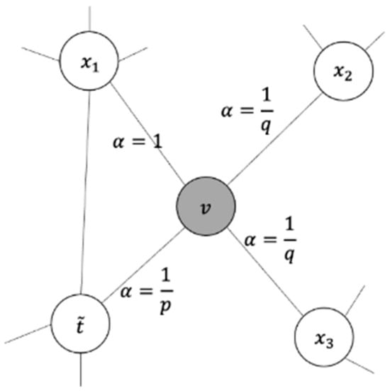
Figure 8. Random walk strategy [17].

The parameter $p$ determines the probability that $v$ will visit the previous node $\tilde{t}$, and $p$ only functions when $d_{\tilde{t}x}$ = 0. The probability of accessing the previous node $\tilde{t}$ is larger if $p$ has a large value. The random walk’s direction is determined by the parameter $q$; $q>1$ causes the random walk to tend nodes near node $\tilde{t}$ (BFS); $q$ only functions when $d_{\tilde{t}x}$ = 2. The random walk has a propensity to travel to nodes far from node $\tilde{t}$ (DFS) if $q<1$. The loss of Node2vec is calculated as (7), where $N_s\left(\tilde{u}\right)$ is the set of neighboring nodes of node $\tilde{u}$ obtained via a sampling strategy, and $f\left(\tilde{u}\right)$ is a mapping function that maps node $\tilde{u}$ to an embedding vector. For the current node $f\left(\tilde{u}\right)$, the optimization goal is to provide each node $f\left(\tilde{u}\right)$ with the condition to maximize the probability of the adjacent node $N_s\left(\tilde{u}\right)$:

$$L_{Node2vec}={max}_f\sum _{u\in V}log\mathrm{Pr}\left( N_s\left(\tilde{u}\right) \right| f\left(\tilde{u})\right)$$

(7)

Then, according to this loss $L_{Node2vec}$, the skip-gram in Word2vec is directly used to learn the embedding vector. The principle of Word2vec is to use the weights of the fully connected layer of a classifier as word vectors. In this classifier, the word’s one-hot vectors are input, then fed into a fully connected layer, and then fed to a SoftMax to obtain the probability of the contexts. We followed a previous work [3] and set $p=q=0.25$. The obtained location-embedding vector is defined as (8), where $\mathbb{g}$ is the dimension of Node2vec output that can be determined, and $B_g$ is the location feature extracted by Node2vec. We use Node2vec to obtain more expressive location features, which fully considers the relationship between each node and its neighbor nodes:

$$Node2vec\left(V,E\right)=B_g^{*}=\left[b_{g_1},b_{g_2},\dots ,b_{g_{\mathbb{g}}}\right], B_g^{*}\in {\mathbb{R}}^{d_{\mathbb{g}}}$$

(8)

4.3.3. Model Structure

We fed the features into the model to obtain the next location. The output of Time2vec is $B_t\in {\mathbb{R}}^{d_h\times d_{\mathbb{t}}}$, and the output of Node2vec $B_g\in {\mathbb{R}}^{d_h\times d_{\mathbb{g}}}$. The semantic $\varsigma$ and user ID $u$ are fed into the fully connected layer to obtain $B_{\varsigma }\in {\mathbb{R}}^{d_h\times d_{\mathbb{s}}}$ and $B_u\in {\mathbb{R}}^{d_h\times d_{\mathbb{u}}}$ as (9), where $W^{\varsigma }\in {\mathbb{R}}^{d_{\varsigma }\times d_{\mathbb{s}}}$ and $W^u\in {\mathbb{R}}^{d_u\times d_{\mathbb{u}}}$ are trainable weight matrices, $b_{\varsigma }$ and $b_u$ are the bias parameters of the fully connected layer. Our prediction model input $\mathit{X}=\left\{{\mathit{X}}_1,{\mathit{X}}_2,\dots ,{\mathit{X}}_h\right\}$ is shown as (10):

$$\begin{gathered} B_{\varsigma }=\varsigma ·W^{\varsigma }+b_{\varsigma } \\ {B}_u=u·W^u+b_u \end{gathered}$$

(9)

$$\begin{gathered} \mathit{X}=concatenate\left[B_t,B_g,B_{\varsigma }\right],\mathit{X}\in {\mathbb{R}}^{d_h\times d} \\ d=d_{\mathbb{t}}+d_{\mathbb{g}}+d_{\mathbb{s}} \end{gathered}$$

(10)

$B_u$ is not directly trained by the prediction model because $B_u$ does not have a time series characteristic; how $B_u$ is considered by the model will be described later. In order to capture long-term dependencies in trajectory sequences, we adopt the Self-Attention model. Self-Attention uses a fully connected layer to consider the information from each step collectively, which allows it to maintain more long-term memory than RNN, which communicates information at each stage. Self-Attention also has fewer parameters and a lower time complexity when compared to RNN. The formula for Self-Attention is shown as (11), where $W^{\mathbb{Q}}\in {\mathbb{R}}^{d\times d_{\mathbb{q}}}, W^{\mathbb{K}}\in {\mathbb{R}}^{d\times d_{\mathbb{k}}}, W^{\mathbb{V}}\in {\mathbb{R}}^{d\times d_{\mathbb{v}}}$ are weight matrices that can be trained. $\mathit{X}$ is fed to three full connections to obtain $\mathbb{Q}\in {\mathbb{R}}^{d_h\times d_{\mathbb{q}}},\mathbb{K}\in {\mathbb{R}}^{d_h\times d_{\mathbb{k}}},\mathbb{V}\in {\mathbb{R}}^{d_h\times d_{\mathbb{v}}}$. $d_{\mathbb{x}}$ ($d_{\mathbb{q}}$ = $d_{\mathbb{k}}$ = $d_{\mathbb{v}}=$ $d_{\mathbb{x}}$) is the dimension of the hidden state of Self-Attention. We then compute the dot product of $\mathbb{Q}$ with ${\mathbb{K}}^T$ (calculate the features similarity of each location in a trajectory sequence), divide by $\sqrt{d_{\mathbb{k}}}$ (the purpose of dividing by $\sqrt{d_{\mathbb{k}}}$ is to make the gradient of SoftMax not too small), apply a SoftMax function (the features similarity of each stage is expressed by probability, and the higher the features’ similarity, the more important the features of the stage), then, dot product $\mathbb{V}$ (obtain a weighted score for each location, which determines which stage features are important) to obtain ${\mathit{X}}^{\mathit{*}}\in {\mathbb{R}}^{d_h\times d_{\mathbb{x}}}$:

$$\begin{gathered} \mathbb{Q}=\mathit{X}·W^{\mathbb{Q}} \\ \mathbb{K}=\mathit{X}·W^{\mathbb{K}} \\ \mathbb{V}=\mathit{X}·W^{\mathbb{V}} \\ {\mathit{X}}^{\mathit{*}}=SoftMax\left(\frac{\mathbb{Q} · {\mathbb{K}}^T}{\sqrt{d_{\mathbb{k}}}}\right)·\mathbb{V} \end{gathered}$$

(11)

Finally, we only take the last stage ${\mathit{X}}_h^{\mathit{*}}\in$ ${\mathit{X}}^{\mathit{*}}$ as the output of Self-Attention, so the dimension of ${\mathit{X}}_h^{\mathit{*}}$ is $1\times d_{\mathbb{x}}$. There are two reasons as to why we only take the last stage ${\mathit{X}}_h^{\mathit{*}}$: Each stage uses the full connection to consider all spatiotemporal contexts of the sequence; if the output is $h$ stages, the number of network parameters will increase, which may easily cause the problem of overfitting.

In order to personalize the prediction model, we consider the user ID in the output of Self-Attention, and then feed it to SoftMax to obtain the final output. The formula is shown as (12), where $W^o\in {\mathbb{R}}^{d_{\mathbb{x}}\times d_{\mathbb{o}}},W^y\in {\mathbb{R}}^{1\times d_g}$ are the weight matrices; $b_o$ and $b_y$ are the bias parameters of the full connection. We feed ${\mathit{X}}_h^{\mathit{*}}$ to the full connection to obtain the output vector $O\in {\mathbb{R}}^{1\times d_{\mathbb{o}}}$. The trajectory patterns of each user are different, and the model may mix them together during training. In order to distinguish the trajectory sequence of each user, $O$ is added to the feature of the user ID $B_u$ to obtain $O_u$, so that the model can distinguish the trajectory pattern of each user. Finally, $O_u$ is fed to the full connection, so that the dimension of the output is the same as the number of grids $g$. After feeding to SoftMax, the final output of the model $y\in {\mathbb{R}}^{1\times d_g}$ can be obtained:

$$\begin{gathered} O={\mathit{X}}_h^{\mathit{*}}·W^o+b_o \\ {O}_u=O+B_u \\ y=SoftMax\left(O_u·W^y+b_y\right) \end{gathered}$$

(12)

5. Experimental Evaluation

This chapter discusses the experiments and examines the results using our model. This chapter is divided into four parts. Our experimental data and setup are covered in great depth in part 1. Part 2 and part 3 are experiments to evaluate the accuracy of our model under numerous parameters while comparing the performance of our model with other models. Part 4 visualizes the next location prediction results.

5.1. Experimental Data and Setting

We use two types of data, which are trajectory data and POI data. The first are trajectory data, and we use Geolife dataset as the trajectory data [26]; the latter are POI data (Beijing city), and we collect these from Tencent Web Service API.

• Trajectory data: Our experiments are performed on the Geolife trajectory dataset. The Geolife dataset was obtained in the Geolife project by 182 users in Beijing over a period of more than 5 years (April 2007 to August 2012). Geolife is characterized by a series of timestamps; each timestamp contains a latitude and longitude, and the dataset contains records of 24,876,978 GPS points. In the stay point detection, the time threshold ${\theta }_t$ is 5 min, and the distance threshold ${\theta }_d$ is 200 m; we then achieve a total of 43,442 stay points. We remove users whose stay point records are less than 200, so the number of users is reduced from 182 to 50, and we will obtain 35,960 stay points. We then build a virtual grid in Beijing and map the coordinates of each stay point to the corresponding grid. The size of the grid is 500 × 500, there are 41,080 grid cells covering Beijing, the number of grid cells that the users have visited is 2211. When generating trajectory sequence, we set the time window to one week and the sliding window to 10. Finally, we obtain 23,775 trajectory sequences. Further details of the preprocessed dataset is shown in Table 2.
  Table 2. Trajectory dataset statistics.

  Attribute	Value
  City	Beijing City
  Duration	April 2007 to August 2012
  Users (raw/processed)	182/50
  GPS points (raw)	24,876,978
  Stay points (raw/processed)	43,442/35,960
  Grid (raw/the users have been)	41,080/2211
  Stay grid (processed)	35,960
  Trajectory sequence (processed)	24,056
  Trajectory sequence/users(processed)	475

• POI data: We obtain the POI data of Beijing from the Tencent Web Service API. They provide detailed POI information such as coordinates, address, ID, name, phone number, type, etc. The Tencent Web Service API divides POIs into 18 main categories, the statistical distribution of which is shown in Figure 9. Therefore, we can calculate the semantic feature vector of each stay point based on these 18 types. In Tencent Maps, “Address” represents natural place names, road names, administrative place names and similar categories. This category does not conflict with other types of POIs.
  

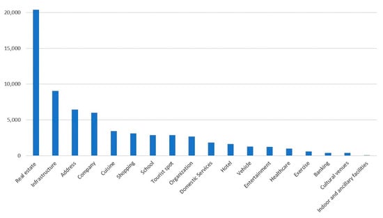  Figure 9. POI category statistics.

As for the experimental settings, all experiments were performed on a computer with Intel Core i9-10900K CPU 3.70 GHz, NVIDIA GeForce RTX 3090, 64GB RAM under Microsoft Windows 10. We divide each trajectory sequence into training and test sets. For each user, we use the first 80% of trajectory sequences as training data and the remaining 20% as testing data. We use Python 3.7 and Keras to put our model into practice. We adopt categorical cross entropy to minimize the loss function, the Adam optimizer is used to train our model, and dropout is used to prevent overfitting. The hidden state d, dropout rate, epoch and the dimensions $d_{\mathbb{t}}, d_{\mathbb{g}},d_{\mathbb{s}} \mathrm{and} d_{\mathbb{u}}$ are set as 64, 0.5, 45 and 20, respectively.

The location prediction is a classification problem; the number of classes is determined by the grid covering the study area (a total of 2211 grids in our study area). Since there are many classes to classify, both prediction accuracy and improvement rate will be low and hard to improve. To evaluate the performance of each method for next location prediction, we evaluate our model with TOP K accuracy (TOP@K), which checks whether the ground-truth location is shown among the Top K result list; the units are percentage points (%), where K = {1, 5, 10, 15}. The evaluation of higher-ranking results is more helpful in practical applications. We train each method 10 times and compute the average accuracy and standard deviation to avoid obtaining good results by training only once.

5.2. Internal Experiment

We conducted seven different internal experiments with different sliding windows, location features, temporal features, semantic features, user features and prediction models. Settings and defaults are listed in Table 3.

Table 3. The settings of internal experiment.

Experiment	Method	Default
Sliding window	Sliding window size = {1, 2, …, 15}	10
Location feature	None/Full connection/Word2vec/Node2vec	Node2vec
Temporal feature	None/Hour/Sin and cos/Time2vec	Time2vec
Semantic feature	Semantic matching k = {1, 2, …, 100}	k = 74
	Closest distance/Semantic matching (not considering home and workplace)/Semantic matching	Semantic Matching
User feature	Remove User ID/Has User ID	Has User ID
Prediction model	LSTM/BiLSTM/Self-Attention	Self-Attention

5.2.1. Time Interval

In this experiment, we compared the trajectory sequence without a time interval setting (Figure 10) to a trajectory sequence with a time interval setting (Figure 11). The trajectory sequence with a time interval setting means that the time interval of each point of a continuous sequence is the same (we set the time interval to 1 h). The trajectory sequence without a time interval setting means that the time interval of each location is inconsistent.

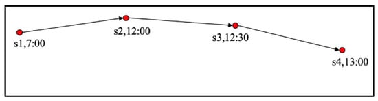
Figure 10. Trajectory sequence without time interval setting.

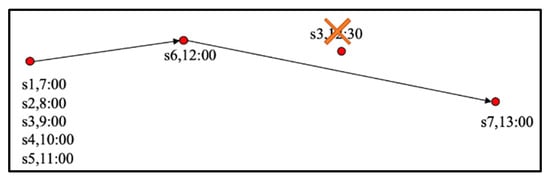
Figure 11. Trajectory sequence with time interval setting.

In Table 4, the two methods differ in how the training data are processed, and the testing data in both methods do not have time interval setting. We can observe that the performance without the time interval setting is better, the main reason is that the time interval setting will generate redundant data; many records of the trajectory sequence are the same location, and it may delete important locations. Furthermore, if the time interval of a location is less than 1 h, this location will be deleted to ensure the same time interval.

Table 4. The TOP@K (%) of different time interval setting.

Method	Top@1	Top@5	Top@10	Top@15
Same time interval	19.88 $\pm$ 0.17	46.55 $\pm$ 0.45	54.68 $\pm$ 0.57	58.71 $\pm$ 0.56
Without time interval	21.56 $\mathbf{\pm }$ 0.45	49.59 $\mathbf{\pm }$ 0.55	58.93 $\mathbf{\pm }$ 0.42	63.05 $\mathbf{\pm }$ 0.52

5.2.2. Sliding Window

Secondly, we performed two experiments to observe the effect of the sliding window size on the model. In the first experiment, we do not set the time window on any of the trajectory sequences to observe the effect of different sliding window sizes on the performance. In the second experiment, we set the time window to observe the different sliding window sizes on the performance. In Figure 12 (Experiment 1), we can see that the accuracy decreases as the sliding window increases. This is because there is no time window setting in this experiment; therefore, the trajectory sequences with long time intervals may occur. This makes it hard to predict the next location. In Figure 13 (Experiment 2), it can be noted that the accuracy increases with the increase in the sliding window; in this experiment, the amount of data decreases as the size of the sliding window increases. This is because if the trajectory sequence length is less than the sliding window size, the trajectory sequence will be deleted. Based on these two experiments, we set the sliding window size $h$ to 10, which not only retains a certain number of trajectory sequences, but also maintains a certain accuracy.

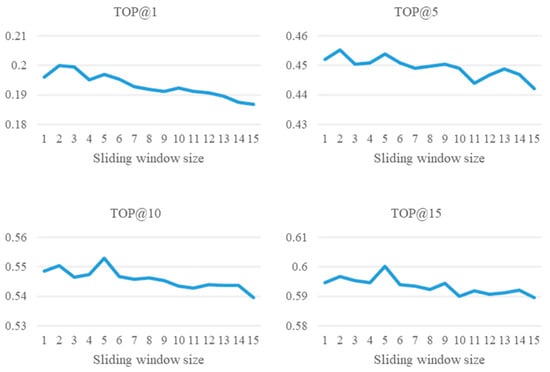
Figure 12. The comparison between different sliding window settings (without the time window).

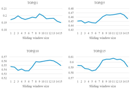
Figure 13. The comparison between different sliding window settings (with the time window).

5.2.3. Location Feature

The third internal experiment pertains to location feature setting. We first test the performance of the model using different location feature extraction methods. Then, we compare FC (Full Connection), Word2vecc and Node2vec. The experiments are shown in Table 5. The results of FC and Word2vec are very similar. Because FC and Word2vec are essentially the same, the difference is that Word2vec is a pre-trained model, and FC is trained in the model. On the other hand, the results of Node2vec are slightly better; Node2vec considers the visiting frequency of nodes while fully considering the relationship between each node and its neighbor nodes; therefore, it allows the model to fully consider the spatiotemporal contexts.

Table 5. The TOP@K (%) of each location feature setting.

Method	Top@1	Top@5	Top@10	Top@15
None	18.32$\pm$0.22	43.07$\pm$0.51	53.23$\pm$0.31	57.89$\pm$0.33
FC	21.31$\pm$0.42	48.89$\pm$0.55	58.24$\pm$0.48	62.34$\pm$0.38
Word2vec	21.37$\pm$0.52	48.78$\pm$0.56	58.28$\pm$0.37	62.31$\pm$0.40
Node2vec	21.56 $\mathbf{\pm }$ 0.45	49.59 $\mathbf{\pm }$ 0.55	58.93 $\mathbf{\pm }$ 0.42	63.05 $\mathbf{\pm }$ 0.52

5.2.4. Temporal Feature

The fourth internal experiment concerns the temporal feature setting, whereby we compare different temporal feature extraction methods (Table 6 lists the experiment results). The first method uses the numbers 1–24 (hours) to represent temporal features. The second method is sin and cos, proposed by Lu et al. [20], whereby the authors had designed the coordinates on a unit circle using the sine and cosine functions to represent the cyclic features of time. In this experiment, using hour or sin and cos does not perform well. Time2vecs performs better because it considers both the original time feature and the periodic feature, which better expresses the periodicity and aperiodicity of time.

Table 6. The TOP@K (%) of each temporal feature setting.

Method	Top@1	Top@5	Top@10	Top@15
None	19.74$\pm$0.39	47.82$\pm$0.49	56.83$\pm$0.36	60.73$\pm$0.50
Hour	20.41$\pm$0.44	47.86$\pm$0.74	56.90$\pm$0.64	60.94$\pm$0.53
Sin and cos	20.78$\pm$0.43	47.66$\pm$0.55	56.67$\pm$0.53	60.62$\pm$0.56
Time2vec	21.56 $\mathbf{\pm }$ 0.45	49.59 $\mathbf{\pm }$ 0.55	58.93 $\mathbf{\pm }$ 0.42	63.05 $\mathbf{\pm }$ 0.52

5.2.5. Semantic Feature

The fifth internal experiment is of the semantic feature setting. Before discussing semantic feature setting, we discuss the impact of semantic matching k. In this experiment, the model only has the semantic feature as input. In Figure 14, we can observe that when k increases, the performance of the prediction model shows an upward trend reaching its peak when k = 73 (so we set k = 73). Based on this experiment result, if the POI distribution around the stay point is considered, the accuracy can be effectively improved. If the closest distance method is used to search for POI (without considering POI distribution), when calculating the semantic vector of the stay point, this method may match the user to a different POI in close proximity instead of the POI which the user has actually visited.

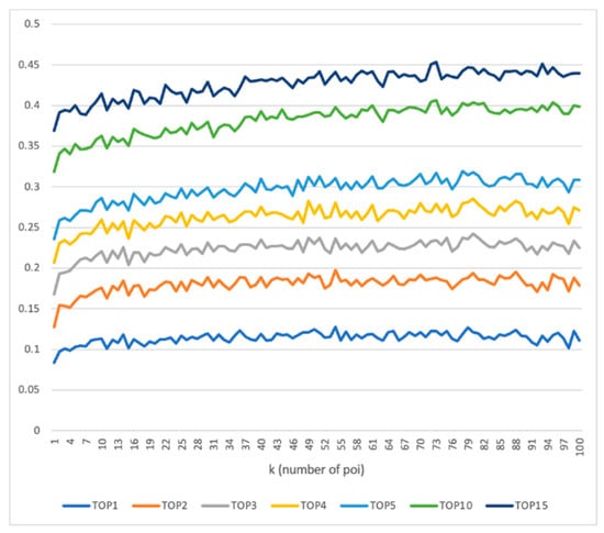
Figure 14. The comparison between different numbers of k (POI).

We perform two experiments to discuss semantic feature setting. In the first experiment, the prediction model only considers the semantic features (Table 7). In the second experiment, all features are used as input for the prediction model (Table 8). We compared: (1) the closest distance (CD), (2) semantic matching without considering home and workplace (SM*) and (3) semantic matching (SM). A comparison of these methods is discussed below:

Table 7. The TOP@K (%) of predicted location only considering semantic feature setting.

Method	Top@1	Top@5	Top@10	Top@15
CD	8.06$\pm$0.32	21.54$\pm$0.27	30.08$\pm$0.33	35.15$\pm$0.28
SM* (Improvement Rate)	9.27$\pm$0.72 (15.01%)	28.32$\pm$0.74 (31.47%)	37.47$\pm$0.79 (24.56%)	42.17$\pm$0.72 (19.97%)
SM (Improvement Rate)	11.75 $\mathbf{\pm }$ 0.31 (45.78%)	30.78 $\mathbf{\pm }$ 0.61 (42.89%)	39.45 $\mathbf{\pm }$ 0.66 (31.15%)	43.87 $\mathbf{\pm }$ 0.66 (24.80%)

Table 8. The TOP@K (%) of each semantic feature setting.

Method	Top@1	Top@5	Top@10	Top@15
None	20.89$\pm$0.52	47.92$\pm$0.45	57.12$\pm$0.47	61.24$\pm$0.54
CD	20.98$\pm$0.45	47.81$\pm$0.61	56.76$\pm$0.57	60.79$\pm$0.52
SM*	21.40$\pm$0.25	48.58$\pm$0.49	58.11$\pm$0.60	62.25$\pm$0.63
SM	21.56 $\mathbf{\pm }$ 0.45	49.59 $\mathbf{\pm }$ 0.55	58.93 $\mathbf{\pm }$ 0.42	63.05 $\mathbf{\pm }$ 0.52

• Comparing SM* with CD: The improvement rate of SM* reaches 15% in TOP@1 (the model only considers semantic features). This shows that if the POI distribution around the stay point is considered, the accuracy can be effectively improved.
• Comparing SM with CD: The improvement rate of SM reaches 45% in TOP@1 (the model only considers semantic features). SM uses sequential pattern mining to compute semantic feature vectors, so that the prediction model can more accurately capture the intent of user activities and achieve better performance.

5.2.6. Prediction Model

The sixth internal experiment concerns the prediction model setting. We compare LSTM, BiLSTM and Self-Attention. LSTM is a variant of the RNN model, which is widely used to handle sequential data; BiLSTM is a combination of backward LSTM and forward LSTM, commonly used to model contextual features. The results are listed in Table 9. We can observe that Self-Attention has an advantage in predicting the next location; this is because Self-Attention is not like RNN-based models, which transmits long-term memory through many stages, thus losing some memory. Instead, the Self-Attention uses full connection to consider each stage in parallel, thus retaining more long-term information.

Table 9. The TOP@K (%) of each prediction model setting.

Method	Top@1	Top@5	Top@10	Top@15
LSTM	21.13$\pm$0.51	48.05$\pm$0.50	57.59$\pm$0.48	61.65$\pm$0.47
BiLSTM	20.82$\pm$0.42	46.71$\pm$0.61	56.12$\pm$0.68	60.30$\pm$0.72
Attention	21.56 $\mathbf{\pm }$ 0.45	49.59 $\mathbf{\pm }$ 0.55	58.93 $\mathbf{\pm }$ 0.42	63.05 $\mathbf{\pm }$ 0.52

5.2.7. User Feature

The last internal experiment is user feature setting. We compared removing a user ID with retaining a user ID. The experimental results are shown in Table 10, which shows that retaining a user ID increases performance while simultaneously personalizing the model.

Table 10. The TOP@K (%) of each user feature setting.

Method	Top@1	Top@5	Top@10	Top@15
Remove User ID	20.52$\pm$0.45	46.77$\pm$0.53	55.28$\pm$0.56	59.22$\pm$0.63
Retain User ID	21.56 $\mathbf{\pm }$ 0.45	49.59 $\mathbf{\pm }$ 0.55	58.93 $\mathbf{\pm }$ 0.42	63.05 $\mathbf{\pm }$ 0.52

5.3. External Experiment

In external experiments, to evaluate the performance of our model, we compare the proposed model with two different models:

• SERM [12]: SERM jointly learns the embedding of various features (location, time, semantic and user) and uses LSTM to predict the next location.
• MSSRM [3]: MSSRM jointly learns various features (user, location and time), uses Node2vec embedding to learn location features and uses Time2vec to learn time features. LSTM is adopted to capture long short-term spatiotemporal dependencies, and Self-Attention is introduced to distinguish each location in different contexts.

We aim to understand the performance of models using LSTM with and without semantic mining. Additionally, we aim to compare the differences between models with and without semantic features. Therefore, in external experiments, the selection of these two methods has been made for comparison. We then perform four external experiments; parameter settings as mentioned in Section 5.1, including comparisons on different methods, grid sizes, sliding window sizes and weekdays/weekends.

5.3.1. Comparison of Different Methods

A comparison of the different methods is shown in Table 11. Based on the results, our method has the best performance amongst the three methods. SERM uses fully connected layers to embed features and does not fully consider information regarding visiting order and visiting frequency; it uses LSTM to predict locations, which may result in information loss when passing on long-term memory due to longer trajectory sequences. The main reason why MSSRM performs worse than our method is because MSSRM does not consider semantic features, thus losing important behavior patterns and living habits information. Our proposed method, on the other hand, effectively extracts semantic features and captures the semantic-awareness spatiotemporal transformation to improve the performance of location prediction.

Table 11. The TOP@K (%) of different methods.

Method	Top@1	Top@5	Top@10	Top@15
SERM	20.03$\pm$0.42	45.58$\pm$0.50	54.80$\pm$0.48	59.02$\pm$0.36
MSSRM	21.03$\pm$0.43	46.93$\pm$0.41	55.88$\pm$0.30	60.00$\pm$0.35
Our Method	21.56 $\mathbf{\pm }$ 0.45	49.59 $\mathbf{\pm }$ 0.55	58.93 $\mathbf{\pm }$ 0.42	63.05 $\mathbf{\pm }$ 0.52

5.3.2. Comparison of Different Methods

The comparison of different grid sizes is shown in Table 12. We compare three different grid sizes (300 × 300, 500 × 500 and 700 × 700). We can observe that the smaller the grid size, the lower the accuracy. This is because as the grid size decreases, the number of locations covered in the study area increases, which makes it difficult to predict the next location. The overall performance: Our Method > MSSRM > SERM.

Table 12. The TOP@K (%) of different grid sizes.

Grid Size (m)	Method	Top@1	Top@5	Top@10	Top@15
300 × 300	SERM	13.82$\pm$0.61	34.93$\pm$0.48	44.22$\pm$0.57	48.71$\pm$0.47
	MSSRM	14.57$\pm$0.49	36.09$\pm$0.37	45.02$\pm$0.47	49.38$\pm$0.46
	Our Method	15.60 $\mathbf{\pm }$ 0.37	39.23 $\mathbf{\pm }$ 0.35	48.45 $\mathbf{\pm }$ 0.51	52.94 $\mathbf{\pm }$ 0.30
500 × 500	SERM	20.03$\pm$0.42	45.58$\pm$0.50	54.80$\pm$0.48	59.02$\pm$0.36
	MSSRM	21.03$\pm$0.43	46.93$\pm$0.41	55.88$\pm$0.30	60.00$\pm$0.35
	Our Method	21.56 $\mathbf{\pm }$ 0.45	49.59 $\mathbf{\pm }$ 0.55	58.93 $\mathbf{\pm }$ 0.42	63.05 $\mathbf{\pm }$ 0.52
700 × 700	SERM	28.89$\pm$0.42	55.36$\pm$0.31	62.98$\pm$0.44	66.79$\pm$0.52
	MSSRM	29.28$\pm$0.61	56.67$\pm$0.52	63.65$\pm$0.41	66.95$\pm$0.57
	Our Method	29.92 $\mathbf{\pm }$ 0.50	58.15 $\mathbf{\pm }$ 0.39	65.04 $\mathbf{\pm }$ 0.47	68.47 $\mathbf{\pm }$ 0.45

5.3.3. Comparison of Different Sliding Window Sizes

The comparison of different sliding window sizes is shown in Table 13. This experiment compares three different sliding window sizes (7, 10 and 13). Based on the table below, when the sliding window size is too large or too small, it is detrimental to the performance. Furthermore, although the sliding window size has an impact on the accuracy, it still does not affect the advantages of our method.

Table 13. The TOP@K (%) of different sliding window sizes.

Window Size	Method	Top@1	Top@5	Top@10	Top@15
7	SERM	$19.77 \pm$0.45	$44.49 \pm$0.66	$53.63 \pm$0.65	$57.86 \pm$0.71
	MSSRM	$20.57 \pm$0.34	$45.80 \pm$0.50	$54.48 \pm$0.34	$58.59 \pm$0.44
	Our Method	$\mathbf{21.31} \mathbf{\pm }$ 0.51	$\mathbf{47.97} \mathbf{\pm }$ 0.27	$\mathbf{57.25} \mathbf{\pm }$ 0.30	$\mathbf{61.33} \mathbf{\pm }$ 0.47
10	SERM	$20.03 \pm$0.42	$45.58 \pm$0.50	$54.80 \pm$0.48	$59.02 \pm$0.36
	MSSRM	$21.03 \pm$0.43	$46.93 \pm$0.41	$55.88 \pm$0.30	$60.00 \pm$0.35
	Our Method	$\mathbf{21.56} \mathbf{\pm }$ 0.45	$\mathbf{49.59} \mathbf{\pm }$ 0.55	$\mathbf{58.93} \mathbf{\pm }$ 0.42	$\mathbf{63.05} \mathbf{\pm }$ 0.52
13	SERM	$19.82 \pm$0.63	$45.38 \pm$0.75	$54.59 \pm$0.72	$58.79 \pm$0.88
	MSSRM	$20.25 \pm$0.59	$45.19 \pm$0.54	$53.66 \pm$0.58	$57.46 \pm$0.58
	Our Method	$\mathbf{20.91} \mathbf{\pm }$ 0.49	$\mathbf{48.17} \mathbf{\pm }$ 0.50	$\mathbf{56.82} \mathbf{\pm }$ 0.54	$\mathbf{60.72} \mathbf{\pm }$ 0.49

5.3.4. Comparison of Different Methods on Weekdays and Weekends

We compared the performance of different methods on weekdays and weekends. Some trajectories cross both weekdays and weekends; we also compared these trajectories together. From Table 14, we can observe that each model performs best on weekdays because most users follow a similar behavior pattern throughout the weekdays, thus their daily life patterns are easier to predict. Our model can perform better than both SERM and MSSRM regardless of weekdays or weekends.

Table 14. The TOP@K (%) of weekdays and weekends.

Date	Method	Top@1	Top@5	Top@10	Top@15
Weekday	SERM	$21.89 \pm$0.45	$48.41 \pm$0.72	$57.57 \pm$0.60	$61.54 \pm$0.61
	MSSRM	$22.36 \pm$0.59	$48.67 \pm$0.84	$57.48 \pm$0.78	$61.57 \pm$0.77
	Our Method	$\mathbf{22.98} \mathbf{\pm }$0.51	$\mathbf{50.84} \mathbf{\pm }$0.83	$\mathbf{60.34} \mathbf{\pm }$0.79	$\mathbf{64.12} \mathbf{\pm }$0.76
Weekend	SERM	$20.25 \pm$1.19	$46.08 \pm$1.54	$56.35 \pm$1.19	$61.22 \pm$0.94
	MSSRM	$19.40 \pm$1.36	$45.53 \pm$1.18	$55.59 \pm$1.19	$60.00 \pm$1.08
	Our Method	$\mathbf{21.58} \mathbf{\pm }$0.82	$\mathbf{51.82} \mathbf{\pm }$1.19	$\mathbf{61.15} \mathbf{\pm }$0.76	$\mathbf{65.29} \mathbf{\pm }$0.66
Cross	SERM	$18.10 \pm$0.49	$42.81 \pm$0.55	$52.29 \pm$0.74	$56.57 \pm$0.48
	MSSRM	$18.57 \pm$0.53	$43.31 \pm$0.50	$52.24 \pm$0.62	$56.37 \pm$0.59
	Our Method	$\mathbf{19.66} \mathbf{\pm }$0.78	$\mathbf{46.26} \mathbf{\pm }$0.84	$\mathbf{55.46} \mathbf{\pm }$0.95	$\mathbf{59.89} \mathbf{\pm }$0.70

5.4. Visualization of Location Prediction Results

We visualize our location prediction model, which is shown in Figure 15. We use the user’s previous ten locations to predict the next location. Each grid has a probability, the redder the grid color indicates a higher probability of being the next location, and the yellow stars refer to the ground truth. The first example A is on the top left of the figure. We can observe that the user is traveling around Kunming Lake (a well-known spot in Beijing). The second example B is on the top right of the figure. The user’s trajectory sequence 1–2 is in Beijing Forestry University. The user then passes through Jianqingyuan Community to reach the China Academy of Building Research (3–5). The user then heads toward the Chinese Academy of Sciences (6–10) and then travels back to the China Academy of Building Research (ground truth). The third example C is on the bottom left of the figure. The user’s trajectory sequence 1–4 is initially in Jianqingyuan residential community (home); after visiting several different places (5–7), the user visits the Chinese Academy of Sciences to study (8–10) and then returns home (ground truth). The last example D is at the bottom right of the figure; the user’s trajectory sequences 1–8 are in the Peking University campus, and the trajectories’ sequence 9–10 and ground truth are in the Tiantongwan community. Based on this trajectory sequence, we can observe that the user returned home to rest after finishing his class at Peking University.

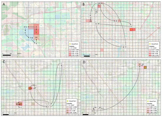
Figure 15. The visualization examples for location prediction, where (A) traveling around Kunming Lake, (B) moving from Beijing Forestry University passes through Jianqingyuan Community to reach the China Academy of Building Research, (C) traveling between home and work and (D) moving from Peking University campus to Tiantongwan community.

6. Conclusions and Future Work

In this paper, we propose a Self-Attention model for Next Location Prediction based on semantic mining. We design a semantic matching method, which considers k-nearest POI, fully considers the spatial features around the stay point and combines sequential pattern mining to result in richer semantic features. To extract spatiotemporal contexts, we use Node2vec and Time2vec, which fully consider the interaction of each location and the periodicity of the time series. Finally, we adopt Self-Attention to capture the spatiotemporal dependencies to predict the next location. Experiments in Geolife show that the semantic matching of this study improved by 45.78% in TOP@1 compared with the closest distance search for POI. In terms of location features and temporal features extraction, TOP@1 has improved by 0.8% and 3.7%, respectively. Compared with the baseline, the model proposed in this paper improved by 2.5% in TOP@1, and improved by 5.6% and 5.0% in TOP@5 and TOP@10, respectively. It can be observed that the accuracy and the improvement rate of the models are quite low, because the location prediction is a classification problem; the number of classes is determined by the grid covering the study area (a total of 2211 grids in our study area). Since there are many categories to classify, the prediction accuracy will be lower.

In the future, we plan to mine other semantic behaviors (not only the home and workplace) and combine them with semantic matching to better understand users’ life patterns. Given the same reciprocal distance when calculating the semantics of each stay point, it can reflect the POI features around a stay point; however, some POI categories with a large number of POIs may occupy most of the weight. In the future, we plan to control the weight of each POI category through the number of POIs in each category. There are also some features that were not considered in this study, such as moving distance or dwelling time; we plan to integrate these features into the model to help the model better learn contextual features. In addition, it is possible to find better neural network models to improve prediction accuracy, such as variants of Attention mechanism and variants of different prediction models (RNN or LSTM). Furthermore, selecting appropriate values for MinPts and the distance threshold (epsilon) in OPTICS can be challenging. Node2Vec requires re-computation for each new set of unknown nodes, and we have not addressed the ‘cold start’ problem in our study. Handling the ‘cold start’ issue will be a part of our future work.

References

- Xu, M.; Han, J. Next Location Recommendation Based on Semantic-Behavior Prediction. In Proceedings of the 5th International Conference on Big Data and Computing, Chengdu, China, 28–30 May 2020; pp. 65–73. [Google Scholar]
- Feng, J.; Li, Y.; Yang, Z.; Qiu, Q.; Jin, D. Predicting Human Mobility with Semantic Motivation via Multi-Task Attentional Recurrent Networks. IEEE Trans. Knowl. Data Eng. 2022, 34, 2360–2374. [Google Scholar] [CrossRef]
- Wen, S.; Zhang, X.; Cao, R.; Li, B.; Li, Y. MSSRM: A Multi-Embedding Based Self-Attention Spatio-Temporal Recurrent Model for Human Mobility Prediction. Hum.-Centric Comput. Inf. Sci. 2021, 11, 37. [Google Scholar] [CrossRef]
- Fernandes, R.; D’Souza GL, R. A New Approach to Predict User Mobility Using Semantic Analysis and Machine Learning. J. Med. Syst. 2017, 41, 188. [Google Scholar] [CrossRef] [PubMed]
- Jiang, J.; Pan, C.; Liu, H.; Yang, G. Predicting Human Mobility Based on Location Data Modeled by Markov Chains. In Proceedings of the IEEE Fourth International Conference on Ubiquitous Positioning, Indoor Navigation and Location Based Services, Shanghai, China, 3–4 November 2016; pp. 145–151. [Google Scholar]
- Xia, Y.; Gong, Y.; Zhang, X.; Bae, H.Y. Location Prediction Based on Variable-order Markov Model and User’s Spatio-Temporal Rule. In Proceedings of the IEEE Conference on Information and Communication Technology Convergence, Jeju Island, Republic of Korea, 17–19 October 2018; pp. 37–40. [Google Scholar]
- Xia, L.; Huang, Q.; Wu, D. Decision Tree-based Contextual Location Prediction from Mobile Device Logs. Mob. Inf. Syst. 2018, 2018, 1852861. [Google Scholar] [CrossRef]
- Al-Molegi, A.; Jabreel, M.; Martínez-Ballesté, A. Move, Attend and Predict: An Attention-Based Neural Model for People’s Movement Prediction. Pattern Recognit. Lett. 2018, 112, 34–40. [Google Scholar] [CrossRef]
- Su, L.; Li, L. Trajectory Prediction Based on Machine Learning. IOP Conf. Ser. Mater. Sci. Eng. 2020, 790, 012032. [Google Scholar] [CrossRef]
- Vaswani, A.; Shazeer, N.; Parmar, N.; Uszkoreit, J.; Jones, L.; Gomez, A.N.; Kaiser, L.; Polosukhin, I. Attention Is All You Need. In Proceedings of the Advances in Neural Information Processing Systems, Long Beach, CA, USA, 4–9 December 2017; pp. 5998–6008. [Google Scholar]
- Wang, S.; Li, A.; Xie, S.; Li, W.; Wang, B.; Yao, S.; Asif, M. A Spatial-Temporal Self-Attention Network (STSAN) for Location Prediction. Complexity 2021, 2021, 6692313. [Google Scholar] [CrossRef]
- Yao, D.; Zhang, C.; Huang, J.; Bi, J. SERM: A Recurrent Model for Next Location Prediction in Semantic Trajectories. In Proceedings of the ACM on Conference on Information and Knowledge Management, Singapore, 6–10 November 2017; pp. 2411–2414. [Google Scholar]
- Zhang, X.; Li, B.; Song, C.; Huang, Z.; Li, Y. SASRM: A Semantic and Attention Spatio-Temporal Recurrent Model for Next Location Prediction. In Proceedings of the IEEE International Joint Conference on Neural Networks, Glasgow, UK, 19–24 July 2020; pp. 1–8. [Google Scholar]
- Ying, J.J.C.; Lee, W.C.; Weng, T.C.; Tseng, V.S. Semantic Trajectory Mining for Location Prediction. In Proceedings of the ACM SIGSPATIAL International Conference on Advances in Geographic Information Systems, Chicago, IL, USA, 1–4 November 2011; pp. 34–43. [Google Scholar]
- Mikolov, T.; Chen, K.; Corrado, G.; Dean, J. Efficient Estimation of Word Representations in Vector Space. arXiv 2013, arXiv:1301.3781. [Google Scholar]
- Sassi, A.; Brahimi, M.; Bechkit, W.; Bachir, A. Location Embedding and Deep Convolutional Neural Networks for Next Location Prediction. In Proceedings of the IEEE 44th LCN Symposium on Emerging Topics in Networking, Osnabrück, Germany, 14–17 October 2019; pp. 149–157. [Google Scholar]
- Grover, A.; Leskovec, J. Node2vec: Scalable Feature Learning for Networks. In Proceedings of the 22nd ACM SIGKDD International Conference on Knowledge Discovery and Data Mining, San Francisco, CA, USA, 13–17 August 2016; pp. 855–864. [Google Scholar]
- Xu, S.; Cao, J.; Legg, P.; Liu, B.; Li, S. Venue2vec: An Efficient Embedding Model for Fine-Grained User Location Prediction in Geo-Social Networks. IEEE Syst. J. 2019, 14, 1740–1751. [Google Scholar] [CrossRef]
- Chen, M.; Zuo, Y.; Jia, X.; Liu, Y.; Yu, X.; Zheng, K. CEM: A Convolutional Embedding Model for Predicting Next Locations. IEEE Trans. Intell. Transp. Syst. 2020, 23, 3349–3358. [Google Scholar] [CrossRef]
- Lu, E.H.C.; Lin, Z.Q. Rental Prediction in Bicycle-Sharing System Using Recurrent Neural Network. IEEE Access 2020, 8, 92262–92274. [Google Scholar] [CrossRef]
- Kazemi, S.M.; Goel, R.; Eghbali, S.; Ramanan, J.; Sahota, J.; Thakur, S.; Wu, S.; Smyth, C.; Poupart, P.; Brubaker, M. Time2vec: Learning A Vector Representation of Time. arXiv 2019, arXiv:1907.05321. [Google Scholar]
- Xie, M.; Yin, H.; Wang, H.; Xu, F.; Chen, W.; Wang, S. Learning Graph-based POI Embedding for Location-Based Recommendation. In Proceedings of the 25th ACM International Conference on Information and Knowledge Management, Indianapolis, IN, USA, 24–28 October 2016; pp. 15–24. [Google Scholar]
- Cao, H.; Xu, F.; Sankaranarayanan, J.; Li, Y.; Samet, H. Habit2vec: Trajectory Semantic Embedding for Living Pattern Recognition in Population. IEEE Trans. Mob. Comput. 2019, 19, 1096–1108. [Google Scholar] [CrossRef]
- Ye, Y.; Zheng, Y.; Chen, Y.; Feng, J.; Xie, X. Mining Individual Life Pattern Based on Location History. In Proceedings of the IEEE Tenth International Conference on Mobile Data Management: Systems, Services, and Middleware, Taipei, Taiwan, 18–20 May 2009; pp. 1–10. [Google Scholar]
- Chen, C.C.; Chiang, M.F. Trajectory Pattern Mining: Exploring Semantic and Time Information. In Proceedings of the IEEE Conference on Technologies and Applications of Artificial Intelligence, Hsinchu, Taiwan, 25–27 November 2016; pp. 130–137. [Google Scholar]
- Zheng, Y.; Xie, X.; Ma, W.Y. GeoLife: A Collaborative Social Networking Service Among User, Location and Trajectory. IEEE Data Eng. Bull. 2010, 33, 32–39. [Google Scholar]
Disclaimer/Publisher’s Note: The statements, opinions and data contained in all publications are solely those of the individual author(s) and contributor(s) and not of MDPI and/or the editor(s). MDPI and/or the editor(s) disclaim responsibility for any injury to people or property resulting from any ideas, methods, instructions or products referred to in the content. |
© 2023 by the authors. Licensee MDPI, Basel, Switzerland. This article is an open access article distributed under the terms and conditions of the Creative Commons Attribution (CC BY) license (https://creativecommons.org/licenses/by/4.0/).