Abstract
Understanding intercity mobility patterns is important for future urban planning, in which the intensity of intercity mobility indicates the degree of urban integration development. This study investigates the intercity mobility patterns of the Greater Bay Area (GBA) in China. The proposed workflow starts by analyzing intercity mobility characteristics, proceeds to model the spatial-temporal heterogeneity of intercity mobility structures, and then identifies the intercity mobility patterns. We first conduct a complex network analysis, based on weighted degrees and the PageRank algorithm, to measure intercity mobility characteristics. Next, we calculate the Normalized Levenshtein Distance for Population Mobility Structure (NLPMS) to quantify the differences in intercity mobility structures, and we use the Non-negative Matrix Factorization (NMF) to identify intercity mobility patterns. Our results showed an evident ‘Core-Periphery’ differentiation characterized by intercity mobility, with Guangzhou and Shenzhen as the two core cities. An obvious daily intercity commuting pattern was found between Guangzhou and Foshan, and between Shenzhen and Dongguan cities at working time. This pattern, however, changes during the holidays. This is because people move from the core cities to peripheral cities at the beginning of holidays and return at the end of holidays. This study concludes that Guangzhou and Foshan have formed a relatively stable intercity mobility pattern, and the Shenzhen–Dongguan–Huizhou metropolitan area has been gradually formed.
1. Introduction
Urban agglomeration has increasingly been a concern for spatial governance and is considered a driving force behind economic growth [1]. As transportation networks become more and more densely woven into urban agglomerations, we may expect urban administrative boundaries to become blurred, leading to urban integration development. Intercity mobility demonstrates the behavior of people leaving the city, where they live for a short time, and moving to other cities in an urban agglomeration. The patterns of intercity mobility have been seen as indictors to measure the degree of urban integration in the urban agglomeration. It is thus important to characterize intercity mobility patterns, to enhance our understanding of the urban connections between cities and to guide the development of new urbanization and transport planning [2].
Many studies on intercity mobility patterns have been conducted, mainly based on self-administered questionnaires [3,4,5] or survey data about the travel behavior of a large group of people [6,7]. Such data have obvious limitations. On the one hand, the reliability of the data is hard to guarantee [8]. On the other hand, it is difficult to obtain sufficient sample data, which limits an in-depth analysis of intercity mobility patterns. To address these issues, some improvements were made, particularly using big data. With the development of technologies, a large number of mobile computing devices with positioning functions have been popularly used to obtain individual positions and track various types of individual movements for a long time with high precision and efficiency [9]. Compared with conventional data sources, big geo-data with position information usually have much finer details at both spatial and temporal dimensions, providing a sophisticated perspective to depict the dynamics of urban activities and the corresponding interactions as well [10].
Nowadays, increasing attention has been paid to using big geo-data to study the interactions between cities. The big geo-data can be roughly divided into three categories according to the different data sources. The first refers to open data derived from government departments, such as high-speed railway operation data [11]. The second refers to mobile signaling data [12]. The third refers to social network data containing location information based on network data mining, such as Weibo check-in data [13] and Baidu index data [14]. Among many, Baidu has been seen as one of the most popular location-based services (LBS) providers in China. Baidu migration data accurately record the movement trajectory of hundreds of millions of people and can reflect people’s behaviors, such as short-term business trips, tourism, family visits, and medical treatments. These data also provide a comprehensive judgment of population flow between cities and their interactions.
With the development of regional integration, the evolution of urban space is moving from “place space” to “flow space”. The introduction of flow space theory [15] has changed the paradigm of urban space research, shifting the static space inside a city to the dynamic connection outside the city. It has laid an important foundation for studying urban networks. For example, some researchers take cities as nodes to form a network for urban agglomerations [16,17,18], to explore the connections between cities or to evaluate each city’s importance based upon the complex network theory [19]. However, such a method mainly analyzes the intercity patterns from the average level at a certain time or stage and fails to effectively characterize the dynamic variations of urban connection. To deal with this issue, existing studies have used singular value decomposition (SVD) [20,21] to characterize the main intracity and intercity mobility patterns. However, one concern is that the obtained decomposition results are not strictly non-negative, leading to interpretability issues. Therefore, these methods are not suited to reveal the mobility patterns intuitively. In addition, previous studies have also shown that intercity mobility patterns differ between different periods. That is, the intercity mobility patterns show obvious temporal heterogeneity. We also witnessed some interesting studies on examining the spatial patterns and determinants of the hukou transfer intention network [22], mapping the intercity mobility patterns at different periods, such as the spring festival travel rush [23], National Day [24], and weekends and weekdays [25]. Few existing studies however, have considered to evaluate the structural differences between intercity mobility patterns during different periods of time.
The aim of this study is to characterize the intercity mobility patterns of cities in an urban agglomeration during different periods and to quantify their structural differences. In the literature, many studies use the Non-negative Matrix Factorization (NMF) for pattern recognition applications [26,27]. However, few studies have been carried out to characterize intercity mobility patterns using NMF in urban agglomerations. An interesting work is by [28], who proposed to compare the structural similarity between Origin-Destination (OD) matrices, i.e., the normalized Levenshtein distance for OD matrices (NLOD). However, little attention has been paid to using the NLOD to quantify the structural difference in intercity mobility patterns during different periods. This study analyzes intercity mobility patterns from both qualitative and quantitative perspectives. The novelty of this paper lies in the following:
- It applies complex network theory to measure the whole characteristics of intercity mobility networks within an urban agglomeration setting;
- It proposes to use the NLOD to model the spatial-temporal heterogeneity for intercity mobility structures, and the NLPMS to quantify the differences in intercity mobility structures within different periods for different cities;
- It identifies intercity mobility patterns during different periods using the NMF method;
2. Materials and Methods
2.1. Study Area and Data
The central government of China has formulated three main development plans regarding urban agglomerations for the Greater Bay Area [29], the Yangtze River Delta [30] and the Beijing–Tianjin–Hebei region [31]. The Greater Bay Area (GBA) is located in the GuangDong Province, China, contributing over 12% of China’s Gross Domestic Product (GDP). It is an advanced version of the Pearl River Delta Urban Agglomeration Initiative. This study chose the Greater Bay Area as our study area, because this region is important for China to build a world-class urban agglomeration as one of the major bay areas in the globe. According to the “Outline Development Plan for the Guangdong-Hong Kong-Macao Greater Bay Area”, by 2035, the region will become a world-class vibrant city cluster and modern economic system. Meanwhile, the GBA has been experiencing a remarkable urbanization process since 1978. It is significant to characterize intercity mobility patterns for promoting the construction of a regional community of mutual benefit and cooperation. Figure 1 provides an overview of the study area, including Foshan, Guangzhou, Jiangmen, Zhaoqing, Zhongshan, Zhuhai, Huizhou, Dongguan, and Shenzhen cities. Due to the difficulty of collecting data in Hong Kong and Macau, these two special administrative regions were not included in this study.
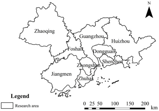
Figure 1.
Overview of the study area in the GBA.
We collected Baidu migration data for each city and obtained the data for 265 days from 14 September 2021 to 5 June 2022 (https://qianxi.baidu.com). The attributes of these data contain the daily flow-in and flow-out scale indexes of each city in the GBA. We obtained 481,770 Baidu migration data records, and then eliminated invalid records. Finally, we obtained a total of 38,160 Baidu migration data records for the study area. The data attributes and examples are listed in Table 1.

Table 1.
Attributes of Baidu migration data.
We multiplied the flow-in scale index by flow-in ratio to represent the daily population movement in each city. The flow-in datasets were obtained by:
where represents the intercity flow-in indicator from one city j to another city i, represents the flow-in ratio from one city j moving into another city i at time , represents the flow-in scale index for this city at time . Likewise, we obtained the flow-out datasets were obtained by:
where represents the intercity flow-out indicator from one city to another city , represents the ratio of the number of people from one city to another city at time , represents the flow-out scale index for this city at time . The whole dataset consists of the flow-in and flow-out datasets.
2.2. Proposed Workflow
The proposed workflow for characterizing intercity mobility patterns is shown in Figure 2. It includes three main steps: (1) measuring the characteristics of intercity mobility networks; (2) quantifying the differences in intercity mobility structures within different periods for different cities; and (3) characterizing intercity mobility patterns during different periods. More specifically, we first formulate two types of matrices: daily intercity mobility OD matrices and time-series intercity mobility flow matrix. We then use complex network analysis methods, based upon weighted degrees and PageRank algorithm, to measure the characteristics of intercity mobility networks. Next, we use the NLPMS, based upon the daily intercity mobility OD matrices, to quantify the differences in intercity mobility structures within different periods for different cities. Last, we use NMF, based upon the time-series intercity mobility flow matrix, to characterize the different intercity mobility patterns during different periods.
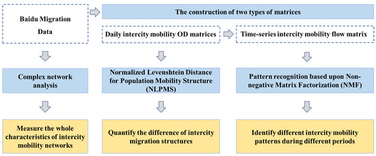
Figure 2.
The proposed workflow for characterizing intercity mobility patterns.
2.3. Research Methods
2.3.1. Complex Network Analysis
We take cities as nodes to formulate the network of urban agglomerations. Then, we build a directed weighted graph to represent the complex intercity mobility network for the urban agglomeration. The relationship between cities is determined to reveal the integration and hierarchy of the network, using weighted degrees and PageRank algorithm. Last, we use a visualization tool in ArcGIS to display the characteristics of intercity mobility networks.
(1) Weighted degrees: We regard a city as a node , where the edge is formed by city and the corresponding flow-in and flow-out source city . The weight of each edge has two types, including and . The weighted degree of city is calculated as follows:
The weighted degree of a city measures the magnitude of the activity in a movement network. The larger the weighted degree is, the more active the city is in the intercity mobility network. Connections between cities are also different. We represent the characteristics of intercity mobility using the grading color drawing function in ArcGIS to visualize the weight of each edge and the weighted degree of each city.
(2) PageRank algorithm: PageRank is a link analysis algorithm and is used to weigh each element of a hyperlinked set of documents, such as the World Wide Web, by measuring its relative importance within the set. We introduced the PageRank algorithm into complex network theory by replacing the page relationship with the city node relationship. It measures the node centrality of the weighted directed network of intercity mobility. A PageRank value describes the importance of each city in the intercity mobility network. The PageRank value is calculated as follows:
where is the PageRank value of node , is a collection of all nodes pointed to node , is the number of links going out of node , and is a damping factor, equal to 0.85 [32].
2.3.2. Construction of Daily Intercity Mobility OD Matrices
To further model the daily intercity mobility structures, based upon the normalized Levenshtein distance for OD matrices (i.e., NLOD), we define a daily intercity mobility OD matrix by constructing the daily intercity OD pairs. The daily intercity mobility OD matrix is defined as:
where represents the intercity flow-out indicator from one city to another city , and represents that the matrix is constructed by the data in .
Each row of the daily intercity mobility OD matrix is independent, and its value represents the flow between the same origin city and different destination cities. The similarity between the daily intercity mobility OD matrices compares the difference of the intercity mobility structure between two different days.
2.3.3. Normalized Levenshtein Distance for Population Mobility Structure
Based upon daily intercity mobility OD matrices, we propose to use the Normalized Levenshtein Distance for Population Mobility Structure (NLPMS) based upon the normalized Levenshtein distance of OD matrices (NLOD), to quantify the differences in intercity mobility structures within different periods for different cities. Below are the main steps in calculating NLPMS:
Step 1:Constructing the population mobility flow sequence from daily intercity mobility OD matrices.
For ith origin city (i ), we construct the population mobility flow sequence from daily intercity mobility OD matrices. Let and be two different population mobility flow sequences starting from city i at two different days. Each consists of a list of flow direction-flow pairs.
Specifically, contains the pair of elements and contains the pair of elements , where indicates the city j starting from city i in , is the intercity flow-out indicator from one city to another city in .
Step 2:Calculating the weighted Levenshtein distance by flow between the population mobility flow sequencesand.
Let and be the descendingly sorted cities of destination locations started from the ith origin city. The weighted Levenshtein distance of the ith origin city by flow is shown in:
The detailed computation of the weighted Levenshtein distance is given in [28].
Step 3:Calculating thestarting from thecity.
where the value of ranges from 0 to 1. The closer is, the intercity mobility structure of the ith origin city between the two days is more similar. That is, the intercity mobility structure is stable between the two days. These values are used to quantify the spatial heterogeneity of intercity mobility structures.
Step 4:Calculating the value of.
Similarly, the value of also ranges from 0 to 1. The closer is, the intercity mobility structure of the whole urban agglomeration between the two days is more similar. These values are used to quantify the temporal heterogeneity of intercity mobility structures.
2.3.4. Construction of Time-Series Intercity Mobility Flow Matrix
Based upon daily intercity mobility OD matrices, we transform the daily intercity mobility OD matrices into a time-series of an intercity mobility flow matrix to characterize intercity mobility patterns. The daily intercity mobility OD matrix is inconvenient to characterize intercity mobility patterns because the time-series mobility patterns are implied in multiple daily intercity mobility OD matrices. However, the row of the time-series intercity mobility flow matrix represents daily intercity mobility indicators between different cities, and the column represents the temporal changes of intercity mobility indicators. The time-series intercity mobility flow matrix is defined as:
where represents the intercity flow-out indicator from one city to another city in . This matrix contains both spatial flow and temporal flow information. It reflects multiple OD states in a continuous period of time and represents the changes of intercity mobility patterns.
2.3.5. Intercity Mobility Pattern Recognition
Based upon time-series intercity mobility flow matrix, we use a rank reduction algorithm to identify the potential intercity mobility patterns. The regular rank reduction algorithms, such as PCA (principal component analysis) [33], ICA (independent component analysis) [34], and SVD (singular value decomposition) [12,20,21] have been widely used to extract a low number of latent components from high-dimensional data. However, traditional rank reduction algorithms can not guarantee the non-negativity of the results, even when the input initial matrix elements are all positive, leading to interpretability issues. Since intercity mobility data are strictly non-negative, Non-negative Matrix Factorization (i.e., NMF) is a compelling alternative for rank reduction [35,36,37]. Therefore, we select NMF to decompose the time-series intercity mobility flow matrix obtained in Section 2.3.4.
The logic of NMF is as follows. Given a time-series intercity mobility flow matrix , , it can be decomposed into a basis matrix and a coefficient matrix using NMF. Here, k is a user-defined variable, called the rank of factorization for NMF, that controls the decomposition dimension. The decomposition is obtained by an optimization process [35,36,37]. The decomposition of the time-series intercity mobility flow matrix based upon NMF is defined as follows:
where is the rank of factorization for NMF. The row vector describes the characteristics of row distribution and the column vector describes the characteristics of column distribution.
The determination of the optimal factor rank affects pattern recognition results [35]. Here, we determine the optimal factor rank k by SVD-NMF, based upon singular value decomposition (i.e., SVD) [36]. For the time-series intercity mobility flow matrix , it can be decomposed into a unitary matrix (with size of m m), a diagonal matrix (with size of m n), and a unitary matrix (with size of n n) using SVD. There exists a factorization with the following form:
where = diag() and the diagonal entries are sorted in descending order. being the singular values with . The diagonal matrix is derived from equation (14). First, we sum all non-zero diagonal entries for , i.e., . According to [36], we use the amount of relatively larger singular values to obtain the rank of factorization k. The rank of factorization k is advocated as being underestimated rather than risking an overestimate [37], and the intercity mobility patterns in the transportation field have strong change rules. Therefore, in this study, the threshold is adjusted to 75%, that is, the result of decomposition contains at least 75% of the information in the time-series intercity mobility flow matrix . It contains enough and sufficient information about the main intercity mobility patterns. In this study, we finally choose the number of singular values that accounts for 75% of all non-zero diagonal entries in the diagonal matrix , the dimension selection rule is defined as follows:
where is the sum of the first singular values after the singular value decomposition of the matrix , i.e., . represents the first singular values after the singular value decomposition of the matrix , i.e., .
3. Results
3.1. The Characteristics of Intercity Mobility Networks
We first calculated the weighted degree and intercity mobility connections of each city in the Greater Bay Area (i.e., GBA). Then, we visualized the characteristics of the intercity mobility networks in the GBA.
We divided the intercity mobility connections between cities in the GBA into five levels, and the weighted degrees of each city were divided into three levels, illustrated in Figure 3. This figure shows that, from the aspect of the weighted degree, the first level refers to Shenzhen and Guangzhou, with a high intensity of intercity mobility. The second level refers to Foshan, Dongguan, and Huizhou, and the remaining cities were concluded into the third level, with a low intensity of intercity mobility. The intercity mobility connections between cities in the GBA are mainly concentrated between three city pairs. The three pairs of cities with the highest degree of connection are Guangzhou–Foshan (a total of 1,415 mobility index), Shenzhen–Dongguan (a total of 1,182 mobility index), and Shenzhen–Huizhou (a total of 713 mobility index). These three city pairs account for only 8.33% of the total number, but the proportion of these three connected intercity mobility flows is 44.87% of the total 36 pairs of connected flows. These three intercity mobility connections represent the main intercity mobility flows in the GBA.
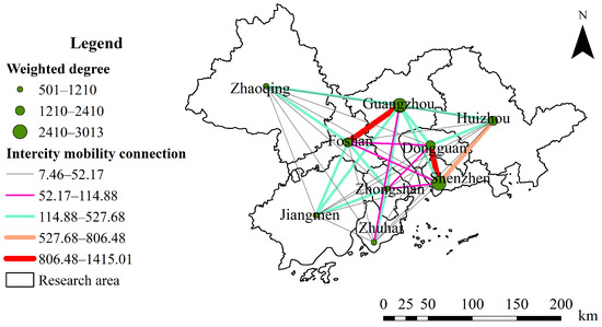
Figure 3.
The ‘Core-Periphery’ differentiation of the GBA.
To sum up, Guangzhou and Shenzhen are the two largest flow-in and flow-out source, showing an obvious “1-n” relationship with a high intensity. There are mainly “1-1” and “1-2” connection patterns, that is, those of Guangzhou–Foshan and Shenzhen–Dongguan–Huizhou.
Table 2 shows the first ninth main intercity population flows of the whole 72 intercity population flows from the perspective of intercity mobility directions. Similarly, the intercity mobility flows from Guangzhou to Foshan ranks first, accounting for 9.648%, while Foshan to Guangzhou ranks second, accounting for 9.530%. Meanwhile, the intercity mobility flows among Shenzhen, Huizhou, and Dongguan ranks 3-8. Obviously, intercity mobility flows among the several cities with perfect comprehensive transportation facilities are active.
Table 2.
Results of complex network analysis of GBA.
Moreover, we calculated the PageRank values of each city to quantify the importance of each city in intercity mobility networks. Guangzhou, Shenzhen, Foshan, and Dongguan rank as the top four. These four cities have higher position in the intercity mobility network of the GBA. It indicates that Huizhou is less important in the GBA than Zhongshan, though Dongguan has a higher weighted degree.
From the perspective of the overall characteristics, the intercity mobility network of the GBA shows an obvious ‘Core-Periphery’ pattern. In the GBA, Guangzhou and Shenzhen are the two core cities. Foshan, Dongguan, and Huizhou are the three periphery cities. The connection between the two core cities becomes weak, which is in line with the integrated development plan of Guangzhou–Foshan and Shenzhen–Dongguan in the GBA. Meanwhile, Huizhou is gradually integrated into the Shenzhen–Dongguan economic development circle. Jiangmen, Zhaoqing, Zhongshan, and Zhuhai need to further accelerate the pace of urban integration development and urban integration. The connections between these cities and the whole urban agglomeration needs to be strengthened.
3.2. The Spatial-Temporal Heterogeneity of Intercity Mobility Structures
To further model the spatial-temporal heterogeneity of the intercity mobility structure, we constructed the daily intercity mobility OD matrices based on the NLOD. Moreover, we used the NLPMS to quantify the differences in intercity mobility structures within different periods for different cities in the GBA.
3.2.1. Construction of Daily Intercity Mobility OD Matrices
We obtained the intercity mobility indicators from one city moving into another. Then, we constructed the daily intercity mobility OD matrices. In total, we obtained 21,465 pairs of related cities, and formed the intercity mobility OD matrices with 9 rows and 9 columns. In total, we constructed 265 daily intercity mobility OD matrices. As shown in Table 3, we selected 1 matrix of the 265 daily intercity mobility OD matrices as an example. It represents the daily intercity mobility structure on 12 October 2021. The first row represents the destination cities. The first column represents the origin cities. The value of the intercity mobility indicator from one city moving into another was filled in the daily intercity mobility OD matrix. The remaining 264 daily intercity mobility OD matrices of other days are similar to this example.
Table 3.
Results of constructing daily intercity mobility OD matrix on 12 October 2021.
3.2.2. The Spatial Heterogeneity of Intercity Mobility Structures
We used the NLPMS to quantify and display the structural differences within the same period’s intercity mobility structure in different cities in the GBA. We calculated the total of 43,956 similarity indexes to reflect the intercity mobility structure in different cities.
As shown in Figure 4, we discovered that different cities show different characteristics in the stability of the intercity mobility structure across one week. That is, the intercity mobility structure in the GBA has obvious spatial heterogeneity. For one thing, box plots of differ obviously in the same city, see Shenzhen. The median of box plots on weekends are much higher than the others on weekdays, the box plots on Fridays are also different from the others on weekdays, and the median of the groups on weekdays are similar, but the spreads of the group on Fridays are more variable. It demonstrates that the intercity mobility structure in Shenzhen on Fridays has some unstable changes. The intercity mobility structure in Shenzhen is stable on weekdays, while it differs on weekends. For another, the boxplots differ between different cities, see Guangzhou and Jiangmen. The spread of the groups in Guangzhou are much smaller than that in Jiangmen. More importantly, the median of the groups in Jiangmen is much higher than that in Guangzhou. It demonstrates that the intercity mobility structure is much more stable than that in Jiangmen. In total, the intercity mobility structure in Guangzhou is the most stable in the GBA, while the intercity mobility structure in Jiangmen changed more frequently over the week than the other cities in the GBA.
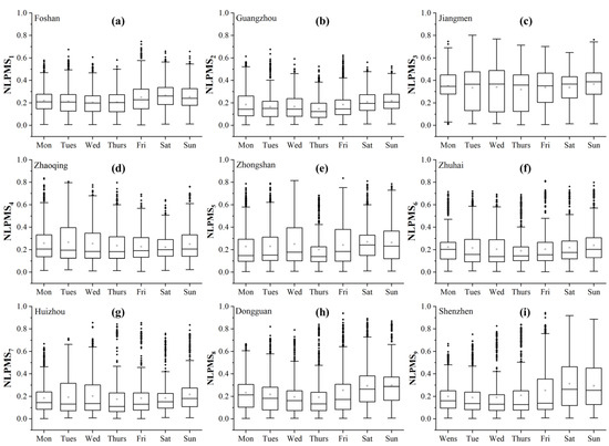
Figure 4.
The spatial heterogeneity of intercity mobility structure in the GBA. (a–i) show differerent characteristics in the stability of the intercity mobility structures across one week in Foshan, Guangzhou, Jiangmen, Zhaoqing, Zhongshan, Zhuhai, Huizhou, Dongguan and Shenzhen, respectively.
In conclusion, the daily stability of the intercity mobility structure is different between cities, meaning that the intercity mobility networks have obvious spatial heterogeneity in the GBA.
3.2.3. The Temporal Heterogeneity of Intercity Mobility Structures
We used the NLPMS to quantify the differences in intercity mobility structures within different periods in the GBA. First, we calculated a total of 69,960 NLPMS of all 265 daily intercity mobility OD matrices two by two, to compare the differences in intercity mobility structure. These NLPMS values reflect two types of the temporal heterogeneity of the intercity mobility structure, including flow-in and flow-out.
As shown in Figure 5a,b, the red color demonstrates that the intercity mobility structure in the GBA differs between the two days. On the contrary, the blue color demonstrates that the intercity mobility structure in the GBA is similar between the two days. According to our statistics, the highest value of the NLPMS is 0.78. During the week, we discovered that the intercity mobility structure is very similar and stable on weekdays, but different on weekends. It implies that the intercity mobility structure differs on weekends from other days in the week. The changes mainly occurred in the following periods shown in Table 4. Especially, this period has eight special time ranges, including Mid-autumn Festival, National Day, New Year’s Day, Chinese New Year, Spring Festival travel period, Qing Ming Festival, Labor Day, and the Dragon Boat Festival. This period also experienced outbreaks of the COVID-19 epidemic in the GBA. Clearly, during these special time ranges, the intercity mobility structure has changed greatly, showing the red color in Figure 5a,b.
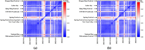
Figure 5.
The temporal heterogeneity of different intercity mobility structures in the GBA. (a) The temporal heterogeneity of flow-in structure. (b) The temporal heterogeneity of flow-out structure.
Table 4.
Descriptions of different holiday periods.
In conclusion, the daily stability of the intercity mobility structure differs during different periods, meaning that the intercity mobility structure has obvious temporal heterogeneity in the GBA.
3.3. Different Intercity Mobility Patterns during Different Periods
Next, we characterized the intercity mobility patterns. As we analyzed in Section 3.2.3, the intercity mobility structure has obvious temporal heterogeneity in the GBA. We constructed the time-series intercity mobility flow matrix and used the NMF method to recognize the different intercity mobility patterns during different periods.
3.3.1. Construction of the Time-Series Intercity Mobility Flow Matrix
We transformed the daily intercity mobility OD matrix into a time-series intercity mobility flow matrix. We constructed a time-series intercity mobility flow matrix with 265 rows and 72 columns. In detail, every city has 8 connections, so the intercity mobility OD matrix has 72 columns. Meanwhile, from 14th September, 2021 to 5th June, a total of 265 days, so that the time-series intercity mobility flow matrix has 265 rows, shown in Table 5. Each row in the matrix represents daily intercity mobility indicators between different cities, and each column represents the temporal changes of intercity mobility indicators.
Table 5.
Results of constructing time-series intercity mobility flow matrix.
3.3.2. Identifying the Different Intercity Mobility Patterns
We used the NMF method to explore the different intercity holiday mobility patterns and intercity daily mobility patterns in the GBA in detail. We extracted the potential intercity holiday mobility patterns from the time-series intercity mobility flow matrix constructed in Section 3.3.1. We selected four as the optimal factoring rank when using the NMF to extract features from the time-series intercity mobility flow matrix. As shown in Table 6, the condition was satisfied when is equal to four. In addition, we conducted a sensitivity analysis for the effect of optimal factor rank k on identifying intercity mobility patterns (see Figures S1–S4 in the Supplementary Material).
Table 6.
Determining the optimal factoring rank k of NMF.
We then visualized the results of the NMF. It should be emphasized that we combined the temporal and spatial distribution to explain the specific meaning of each intercity mobility pattern. The values of temporal flow represent the degree of fluctuation in the intercity mobility population patterns in the time dimension. The values of spatial flow represent the fluctuation direction in the intercity mobility population patterns in the spatial dimension. The sudden change in direction in the temporal distribution flow acts on the intercity flow direction with a darker color in the spatial distribution flow.
As shown in Figure 6c, the light red bar denotes the weekend periods and the light purple bar denotes the holiday periods in the line chart, including the Mid-autumn Festival, National Day, New Year’s Day, Chinese New Year, Spring Festival travel period, Qing Ming Festival, Labor Day, and the Dragon Boat Festival.
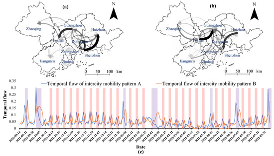
Figure 6.
The intercity holiday mobility patterns in the GBA. (a) Spatial flow in intercity mobility pattern A. (b) Spatial flow in intercity mobility pattern B. (c) Temporal flow in intercity mobility patterns A and B. The light red bar denotes the weekend periods, and the light purple bar denotes the holiday periods, respectively.
We found that there are two types of intercity mobility patterns, A and B, during holiday periods, including two directions of intercity mobility. The flow of people from the core cities to the non-core cities generally reaches the peak on the day before, or on the first day of the small and long holidays, and then quickly flows from the non-core cities to the core cities and reaches the peak of return on the last day of the small and long holidays. More specifically, a large number of citizens migrate from Guangzhou to Foshan, and from Shenzhen to Huizhou or Dongguan. For another, at the end of weekends or holidays, the intercity mobility flows from Foshan to Guangzhou and from Huizhou to Shenzhen show a remarkable increasing trend.
We discovered two main intercity mobility patterns, C and D, and two main connections on weekdays: Guangzhou–Foshan and Shenzhen–Dongguan. As shown in Figure 7, compared to the intercity mobility patterns during the holiday periods, the intercity mobility patterns during usual periods have a smaller fluctuation and a stabler intercity mobility structure. Specifically, Guangzhou–Foshan and Shenzhen–Dongguan have strong mobility connections. The daily population flow is relatively stable due to the need for daily cross-city commuting on weekdays, which shows the urban integration effect. Significantly, the population flow in these two intercity mobility patterns has a slight fluctuation due to the COVID-19 outbreak. However, the COVID-19 pandemic does not change the whole daily intercity mobility patterns in the GBA.
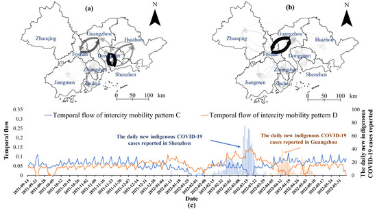
Figure 7.
The intercity daily mobility patterns in the GBA. (a) Spatial flow in intercity mobility pattern C. (b) Spatial flow in intercity mobility pattern D. (c) Temporal flow in intercity mobility patterns C and D. The blue bar and orange bar denotes the daily new indigenous COVID-19 cases reported in Shenzhen and Guangzhou, respectively.
All in all, the intercity mobility structure between the core cities and periphery cities shows a cyclical change during the “week”, and there is a pendulum phenomenon around the weekend. The intercity mobility rule in one week is that the intercity mobility structure has a smaller fluctuation from Tuesday to Thursday and that most of them are daily intercity commuting. On the other hand, Fridays and Saturdays are the peak times when the population of the core cities flows to the non-core cities. On Sundays and Mondays, a large number of people return to the core cities, so as to achieve the dynamic balance of regional population flow. This phenomenon can be called “the pendulum phenomenon of weekends” [38].
4. Discussion
This study measures the characteristics of intercity mobility networks in the Greater Bay Area (i.e, GBA), and quantifies the differences in intercity mobility structures within different periods for different cities. Our first finding is that using a complex network analysis on the Baidu migration data can effectively reflect the characteristics of intercity mobility networks in the GBA. It is characterized by the ‘Core-Periphery’ differentiation. This enhances our understanding of the connection among cities in the GBA from the perspective of intercity mobility flow. The second finding is that the Normalized Levenshtein distance for Population Mobility Structure (i.e, NLPMS), based on normalized Levenshtein distance for OD matrices (i.e, NLOD), is appliable to quantify the structural differences in intercity mobility structures. This expands the applications of the NLOD proposed in [28]. The third finding is that the Non-negative Matrix Factorization (NMF) can intuitively extract the potential intercity mobility patterns. This fills in the gaps that other decomposition methods leave, producing less interpretable results as given in [20,21]. This study provides a systematic workflow to characterize the intercity mobility patterns for the GBA in China, especially from the perspective of intercity population mobility flow.
A complex network analysis method is popularly used for urban studies. We used this method to analyze Baidu migration data in the GBA. Both results of our study and Qiu’s study [38] show that the GBA exhibits a ‘Core-Periphery’ differentiation structure. Benefiting from the urban integration development policy with Guangzhou and Shenzhen as the two core cities, Foshan, Dongguan, and Huizhou adjacent to the two core cities, have a large scale of mobility. The difference is that their results showed that the connection of transport flow between Guangzhou and Shenzhen was strong. However, according to our research, we found that the connection between Guangzhou and Shenzhen was weak (see in Figure 3). This suggests that the transport flow based on the frequency of the transport, such as public buses, which have fixed departure times but do not necessarily reflect the intensity of the connection between the two cities. It is relatively affected by traffic schedules. By contrast, the mobility scale is a more direct reflection and indicator. In addition, with the development of urban construction, the dual center pattern is gradually formed. The connection of the intercity mobility flow between two core cities becoming weak is reasonable. The intercity mobility network of the GBA is not mature enough, other non-core cities contain great contact strength and development potential although Dongguan and Foshan will gradually become a sub center of intercity mobility. The GBA needs to give full play to the radiation and drive roles of the hubs and core nodes and clarify the division of regional functions, in order to promote the development of regional linkage structures.
According to existing studies [23,24,25], the intercity mobility structure varies between periods. That is, the intercity mobility structure has obvious spatial-temporal heterogeneity. We proposed to use the NLPMS based on the NLOD to display the spatial-temporal heterogeneity of the intercity mobility structure, and Figure 5 provides a visual representation of the spatial-temporal heterogeneity in the intercity mobility structure with a quantitative indicator. This result means that the intercity mobility structure is effectively influenced by holidays in the different cities in the GBA. This study demonstrated the validity of using NLPMS to quantify the differences in intercity mobility structures across different periods for different cities. Moreover, we can also model in the future research, the spatial-temporal heterogeneity of the intercity mobility structure based upon multi-source data. Such research would be helpful to make up the limitations of a single data source.
NMF has been a great contribution to image analysis and processing areas. The intercity mobility data can be transformed into one matrix, forming one image. In this context, we can use NMF to extract the different intercity mobility patterns during different periods, which was not used in the previous study about the GBA. We found that the intercity mobility structure in the GBA contains various types of intercity mobility patterns (see in Figure 6 and Figure 7). Similar to Yang’s [17] and Chen’s [39] studies on other urban agglomerations, intercity employment has created the phenomenon of intercity commuting. The commuting cycle contains “one-day commuting” and “one week commuting”, reflecting the separation of work and housing between cities and the combination of work and housing within the region. In the GBA, this phenomenon mainly shows in two connections, including Guangzhou–Foshan and Shenzhen–Dongguan. It reflects the effect of urban integration development in Guangzhou–Foshan and Shenzhen–Dongguan. Our study plays an important role in the planning of constructing the transport. The GBA needs to accelerate the integrated construction of transportation and improve the connection of intercity roads, especially between Shenzhen and Huizhou, to promote regional integration and coordinated development. Moreover, according to our analysis, we found that there is a clear time-space characteristic law for the change of the intercity mobility flow with the effect of urban integration. In further work, the supply of intercity transportation can be flexibly adjusted according to the time change of movement heat, by predicting the peak and trough of intercity mobility at a specific time, so as to promote the efficient use of intercity transportation and meet the large intercity mobility demand. Meanwhile, it should be noted that the key to NMF is to determine the optimal factor rank k, which is both difficult and uncertain [35]. The choice of different values has a great influence on the decomposition results. It is necessary to determine the NMF dimension and threshold according to the specific needs of research. For further research, it remains an important topic to investigate the determination of the optimal factor rank k when using the method of NMF.
5. Conclusions
This study characterized the intercity mobility patterns of the urban agglomeration based on Baidu migration data. We proposed a systematic workflow to explore the intercity mobility networks of the urban agglomeration. We used the Greater Bay Area (GBA) in China as an example. The following conclusions can be drawn:
- Using the complex network analysis, the intercity mobility in the GBA is characterized by the ‘Core-Periphery’ differentiation with Guangzhou and Shenzhen as the two core cities;
- Based on Baidu migration data, Normalized Levenshtein distance for Population Mobility Structure (NLPMS) can effectively quantify the structural differences in intercity mobility structures for cities within different periods in the GBA;
- The Non-negative Matrix Factorization (NMF) method can be used to explore the different intercity mobility patterns during different periods in the GBA;
- The intercity mobility patterns showed that Guangzhou and Foshan, and Shenzhen and Dongguan were connected with obvious urban integration development features.
Our results contribute to characterizing the intercity mobility patterns for the Greater Bay Area in China, which play a vital role in guiding the development of new urbanization and transport planning. Moreover, our systematic workflow could be applied to many other urban agglomerations.
Supplementary Materials
The following supporting information can be downloaded at: https://www.mdpi.com/article/10.3390/ijgi12010005/s1. Figure S1. Changes of singular values and Mean Square Error related to k. (a) Changes of singular values. (b) Changes of Mean Square Error compared with the origin matrix; Figure S2. The intercity mobility pattern in the GBA when k = 1. (a) Spatial flow of intercity mobility pattern A. (b) Temporal flow of intercity mobility pattern A.; Figure S3. The intercity mobility patterns in the GBA when k = 2. (a) Spatial flow of intercity mobility pattern A. (b) Spatial flow of intercity mobility pattern B. (c) Temporal flow of intercity mobility pattern A. (d) Temporal flow of intercity mobility pattern B; Figure S4. The intercity mobility patterns in the GBA when k = 3. (a) Spatial flow of intercity mobility pattern A. (b) Spatial flow of intercity mobility pattern B. (c) Spatial flow of intercity mobility pattern C. (d) Temporal flow of intercity mobility pattern A. (e) Temporal flow of intercity mobility pattern B. (f) Temporal flow of intercity mobility pattern C.1
Author Contributions
Conceptualization, Yanzhong Yin and Qunyong Wu; methodology, Yanzhong Yin; visualization, Yanzhong Yin; writing— original draft preparation, Yanzhong Yin; writing—review and editing, Qunyong Wu and Mengmeng Li; All authors have read and agreed to the published version of the manuscript.
Funding
National Nature Science Foundation of China (Grant number No. 41471333) and National Nature Science Foundation of China (Grant number No. 42201500).
Institutional Review Board Statement
Not applicable.
Informed Consent Statement
Not applicable.
Data Availability Statement
Not applicable.
Conflicts of Interest
The authors declare no conflict of interest.
References
- Liu, Y.; Zhang, X.; Pan, X.; Ma, X.; Tang, M. The spatial integration and coordinated industrial development of urban agglomerations in the Yangtze River Economic Belt, China. Cities 2020, 104, 102801. [Google Scholar] [CrossRef]
- Aunan, K.; Wang, S. Internal migration and urbanization in China: Impacts on population exposure to household air pollution (2000–2010). Sci. Total Environ. 2014, 481, 186–195. [Google Scholar] [CrossRef] [PubMed]
- Cervero, R.; Landis, J. Suburbanization of jobs and the journey to work: A submarket analysis of commuting in the San Francisco Bay Area. J. Adv. Transp. 1992, 26, 275–297. [Google Scholar] [CrossRef]
- Næss, P.; Røe, P.G.; Larsen, S. Travelling distances, modal split and transportation energy in thirty residential areas in Oslo. J. Environ. Plan. Manag. 1995, 38, 349–370. [Google Scholar] [CrossRef]
- Cervero, R. Traditional neighborhoods and commuting in the San Francisco Bay Area. Transportation 1996, 23, 373–394. [Google Scholar] [CrossRef]
- Gonzalez, M.C.; Hidalgo, C.A.; Barabasi, A.L. Understanding individual human mobility patterns. Nature 2008, 453, 779–782. [Google Scholar] [CrossRef]
- Garske, T.; Yu, H.; Peng, Z.; Ye, M.; Zhou, H.; Cheng, X.; Wu, J.; Ferguson, N. Travel patterns in China. PLoS ONE 2011, 6, e16364. [Google Scholar] [CrossRef]
- Stead, D.; Marshall, S. The relationships between urban form and travel patterns. An international review and evaluation. Eur. J. Transport. Infrastruct. 2001, 1, 113–141. [Google Scholar]
- Lu, Y.; Liu, Y. Pervasive location acquisition technologies: Opportunities and challenges for geospatial studies. Comput. Environ. Urban. Syst. 2012, 36, 105–108. [Google Scholar] [CrossRef]
- Wan, L.; Gao, S.; Wu, C.; Jin, Y.; Mao, M.; Yang, L. Big data and urban system model-substitutes or complements? A case study of modelling commuting patterns in Beijing. Comput. Environ. Urban. Syst. 2018, 68, 64–77. [Google Scholar] [CrossRef]
- Hu, H.; Huang, X.; Li, P.; Zhao, P. Comparison of network structure patterns of urban agglomerations in China from the perspective of space of flows: Analysis based on railway schedule. J. Geo-Inf. Sci. 2022, 24, 1525–1540. [Google Scholar]
- Li, Z.; Sun, H.; Li, L. Analysis of intercity travel in the Yangtze River Delta based on mobile signaling data. J. Tsinghua Univ. Sci. Technol. 2022, 62, 1203–1211. [Google Scholar] [CrossRef]
- Li, A.; Mou, N.; Zhang, L.; Yang, T.; Liu, W.; Liu, F. Tourism flow between major cities during China’s national day holiday: A social network analysis using weibo check-in data. IEEE Access 2020, 8, 225675–225691. [Google Scholar] [CrossRef]
- Liu, Y.; Liao, W. Spatial Characteristics of the Tourism Flows in China: A Study Based on the Baidu Index. ISPRS Int. J. Geo-Inf. 2021, 10, 378. [Google Scholar] [CrossRef]
- Castells, M. The Space of Flows. In The Rise of the Network Society; Wiley-Blackwell: Oxford, UK, 2010; ISBN 978-1-4443-1951-4. [Google Scholar]
- Wang, N.; Chen, R.; Zhao, Y. Analysis of the provincial information space network basted on the internet information flow. Geogr. Res. 2016, 35, 137–147. [Google Scholar]
- Yang, Z.; Hua, Y.; Cao, Y.; Zhao, X.; Chen, M. Network Patterns of Zhongyuan Urban Agglomeration in China Based on Baidu Migration Data. ISPRS Int. J. Geo-Inf. 2022, 11, 62. [Google Scholar] [CrossRef]
- Jiang, H.; Luo, S.; Qin, J.; Liu, R.; Yi, D.; Liu, Y.; Zhang, J. Exploring the Inter-Monthly Dynamic Patterns of Chinese Urban Spatial Interaction Networks Based on Baidu Migration Data. ISPRS Int. J. Geo-Inf. 2022, 11, 486. [Google Scholar] [CrossRef]
- Li, C.; Wu, Z.; Zhu, L.; Liu, L.; Zhang, C. Changes of spatiotemporal pattern and network characteristic in population flow under COVID-19 epidemic. ISPRS Int. J. Geo-Inf. 2021, 10, 145. [Google Scholar] [CrossRef]
- Duan, Z.; Lei, Z.; Zhang, M.; Li, H.; Yang, D. Understanding multiple days’ metro travel demand at aggregate level. IET Intell. Transport. Syst. 2019, 13, 756–763. [Google Scholar] [CrossRef]
- Wang, Z.; Nie, W.; Lin, T. Analysis of the spatio-temporal characteristics of intercity travel based on SVD and complex network: Take Bohai Rim City Group as an example. In Proceedings of the International Conference on Intelligent Traffic Systems and Smart City (ITSSC 2021) SPIE, Zhengzhou, China, 19–21 November 2021; Volume 12165, pp. 357–365. [Google Scholar]
- Gu, H.; Liu, Z.; Shen, T. Spatial pattern and determinants of migrant workers’ interprovincial hukou transfer intention in China: Evidence from a National Migrant Population Dynamic Monitoring Survey in 2016. Popul. Space Place 2020, 26, e2250. [Google Scholar] [CrossRef]
- Lai, J.; Pan, J. Spatial pattern of population flow among cities in China during the spring festival travel rush based on “Tencent migration” data. Hum. Geogr. 2019, 34, 108–117. [Google Scholar] [CrossRef]
- Pan, J.; Lai, J. Spatial pattern of population mobility among cities in China: Case study of the National Day plus Mid-Autumn Festival based on Tencent migration data. Cities 2019, 94, 55–69. [Google Scholar] [CrossRef]
- Cui, C.; Wu, X.; Liu, L.; Zhang, W. The spatial-temporal dynamics of daily intercity mobility in the Yangtze River Delta: An analysis using big data. Habitat Int. 2020, 106, 102174. [Google Scholar] [CrossRef]
- Aledavood, T.; Kivimäki, I.; Lehmann, S.; Saramäki, J. Quantifying daily rhythms with non-negative matrix factorization applied to mobile phone data. Sci. Rep. 2022, 12, 1–10. [Google Scholar] [CrossRef] [PubMed]
- Gao, Y.; Liu, J.; Xu, Y.; Mu, L.; Liu, Y. A spatiotemporal constraint non-negative matrix factorization model to discover intra-urban mobility patterns from taxi trips. Sustainability 2019, 11, 4214. [Google Scholar] [CrossRef]
- Behara, K.N.S.; Bhaskar, A.; Chung, E. A novel approach for the structural comparison of origin-destination matrices: Levenshtein distance. Transp. Res. Part. C Emerg. Technol. 2020, 111, 513–530. [Google Scholar] [CrossRef]
- Zhang, Q.; Cai, X.; Liu, X.; Yang, X.; Wang, Z. The Influence of Urbanization to the Outer Boundary Ecological Environment Using Remote Sensing and GIS Techniques—A Case of the Greater Bay Area. Land 2022, 11, 1426. [Google Scholar]
- Xie, H.; Ouyang, Z.; Choi, Y. Characteristics and influencing factors of green finance development in the Yangtze river delta of China: Analysis based on the spatial durbin model. Sustainability 2020, 12, 9753. [Google Scholar] [CrossRef]
- Wang, D.; Sun, Z.; Chen, J.; Wang, X.; Zhang, X.; Zhang, W. Analyzing the interpretative ability of landscape pattern to explain thermal environmental effects in the Beijing-Tianjin-Hebei urban agglomeration. PeerJ 2019, 7, e7874. [Google Scholar] [CrossRef]
- Brin, S.; Page, L. The anatomy of a large-scale hypertextual web search engine. Comput. Netw. ISDN Syst. 1998, 30, 107–117. [Google Scholar] [CrossRef]
- Chang, L.C.; Liou, J.Y.; Chang, F.J. Spatial-temporal flood inundation nowcasts by fusing machine learning methods and principal component analysis. J. Hydrol. 2022, 612, 128086. [Google Scholar] [CrossRef]
- Lassance, N.; DeMiguel, V.; Vrins, F. Optimal portfolio diversification via independent component analysis. Oper. Res. 2022, 70, 55–72. [Google Scholar] [CrossRef]
- Gillis, N. The why and how of nonnegative matrix factorization. arXiv 2014, arXiv:1401.5226. [Google Scholar]
- Qiao, H. New SVD based initialization strategy for non-negative matrix factorization. Pattern Recognit. Lett. 2015, 63, 71–77. [Google Scholar] [CrossRef]
- Huffman, M.; Davis, A.; Park, J.; Curry, J. Identifying Population Movements with Non-Negative Matrix Factorization from Wi-Fi User Counts in Smart and Connected Cities. arXiv 2021, arXiv:2111.10459. [Google Scholar]
- Qiu, J.; Liu, Y.; Chen, H.; Gao, F. Spatial Network Pattern of Guangdong-Hong Kong-Macao Greater Bay Area from the Perspective of Space of Flows—A Comparative Analysis Based on Information Flow and Traffic Flow. Econ. Geogr. 2019, 39, 7–15. [Google Scholar] [CrossRef]
- Chen, S.; Shen, L. Study on spatial-temporal characteristics of population mobility in the urban integration areas of three cities based on Tencent location big data. Mod. Urban. Res. 2019, 11, 2–12. [Google Scholar]
Disclaimer/Publisher’s Note: The statements, opinions and data contained in all publications are solely those of the individual author(s) and contributor(s) and not of MDPI and/or the editor(s). MDPI and/or the editor(s) disclaim responsibility for any injury to people or property resulting from any ideas, methods, instructions or products referred to in the content. |
© 2022 by the authors. Licensee MDPI, Basel, Switzerland. This article is an open access article distributed under the terms and conditions of the Creative Commons Attribution (CC BY) license (https://creativecommons.org/licenses/by/4.0/).