
Canopy Assessment of Cycling Routes: Comparison of Videos from a Bicycle-Mounted Camera and GPS and Satellite Imagery

Abstract
1. Introduction
Research Objectives
2. Materials and Methods
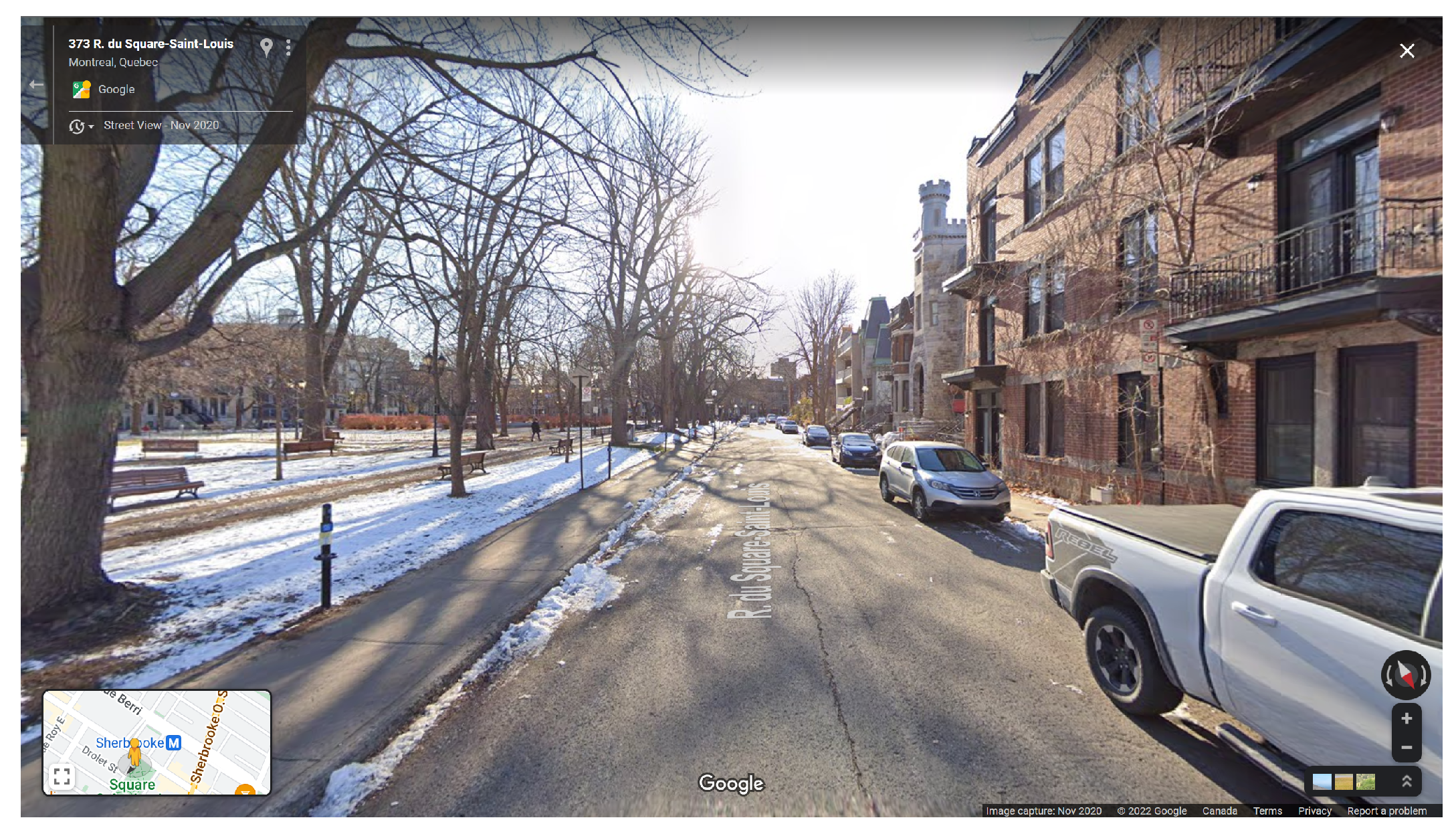
2.1. Study Area and Primary Data Collection
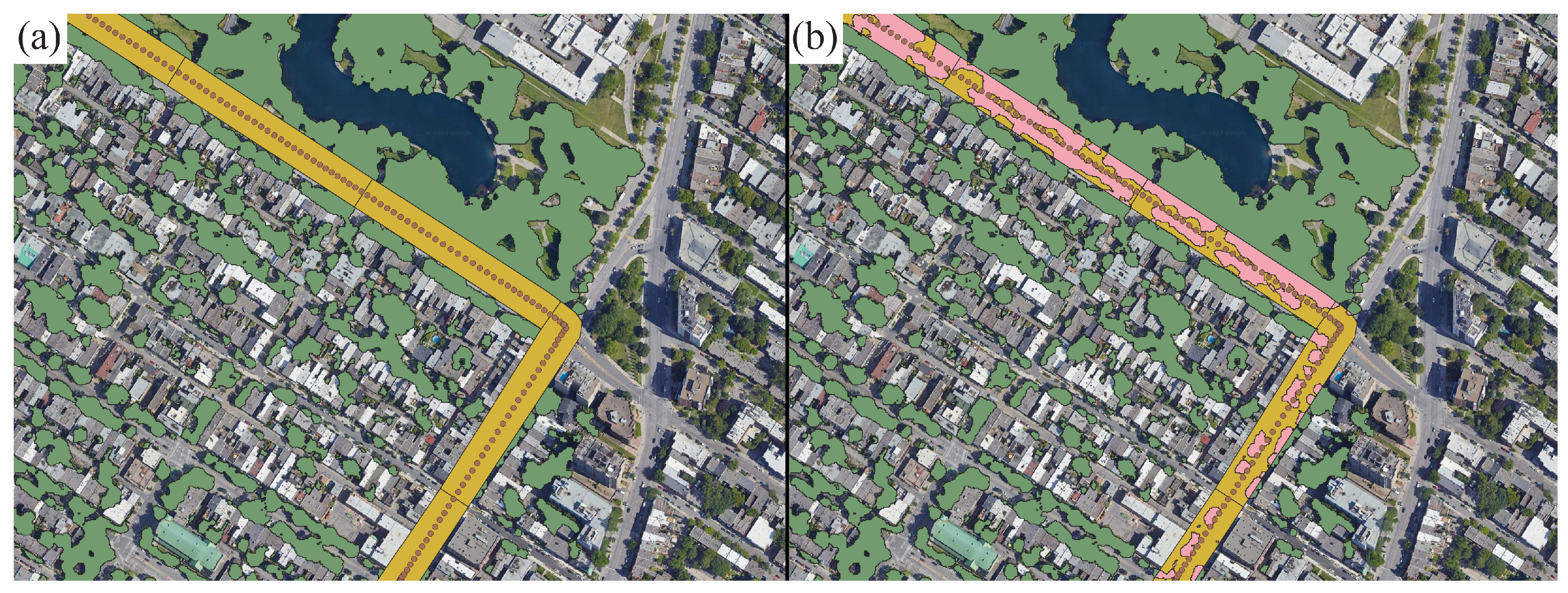
2.2. GIS Secondary Data on Road Network and Canopy
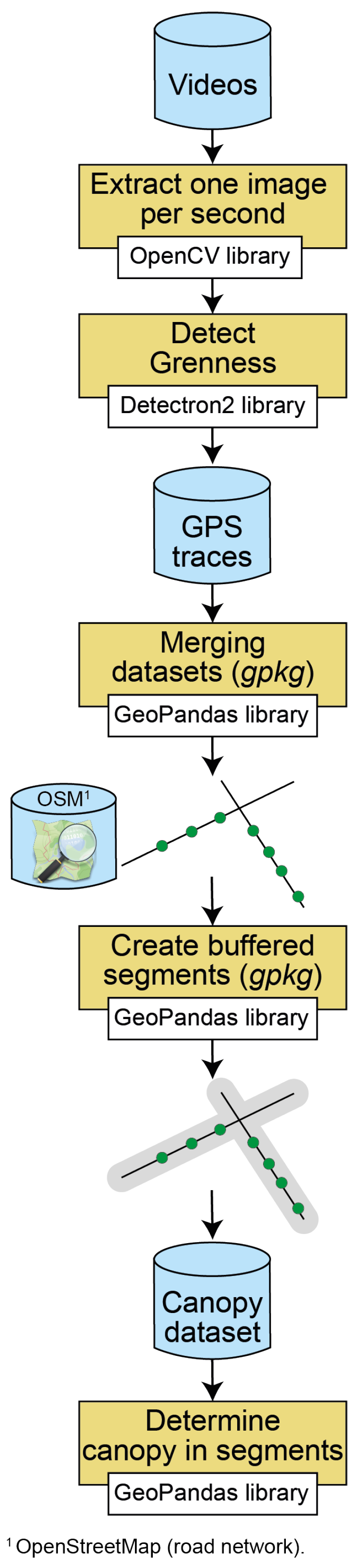
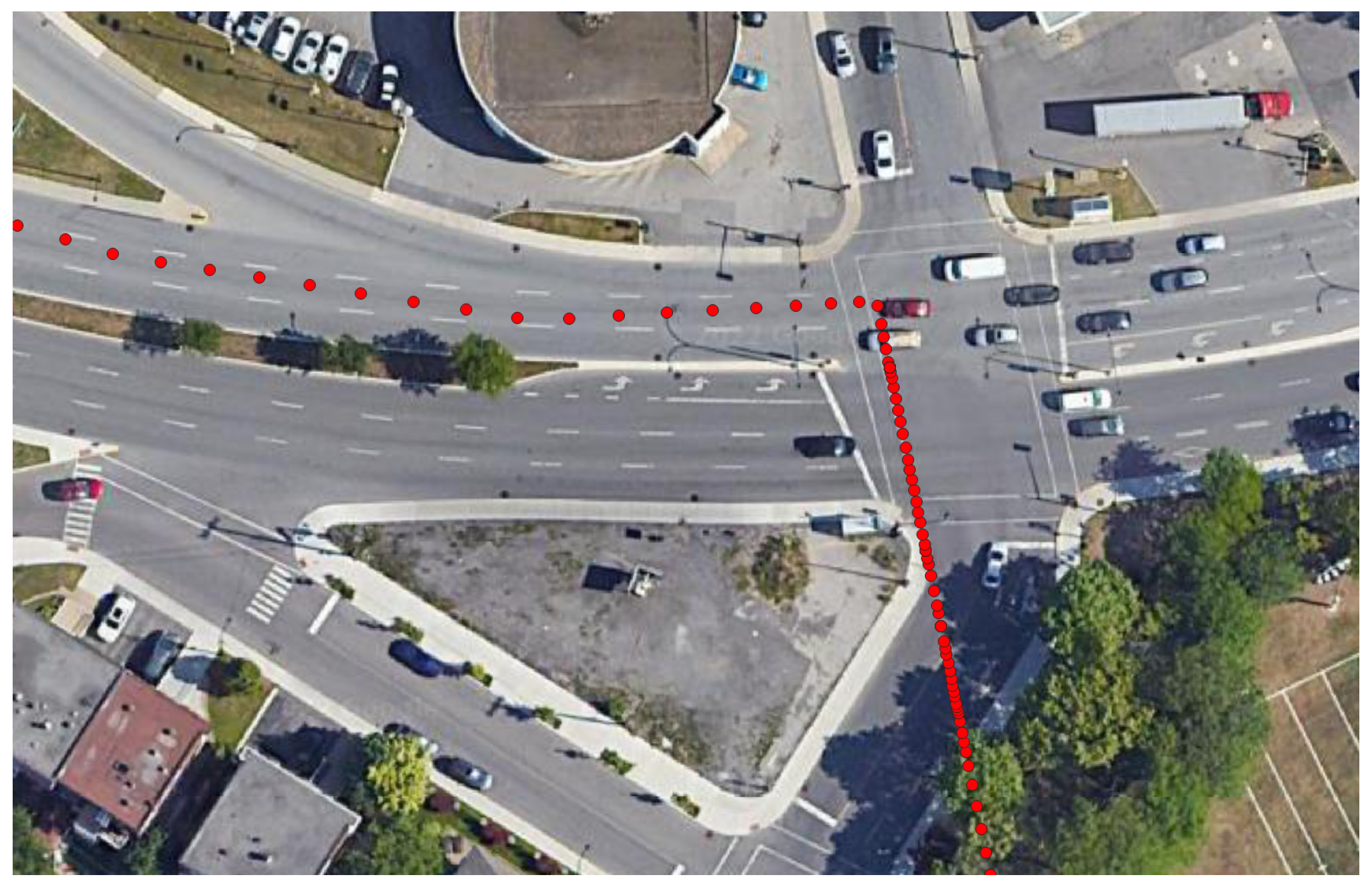
2.3. Data Processing
2.4. Data Analysis
3. Results
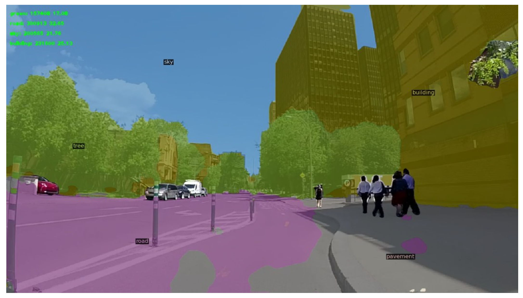
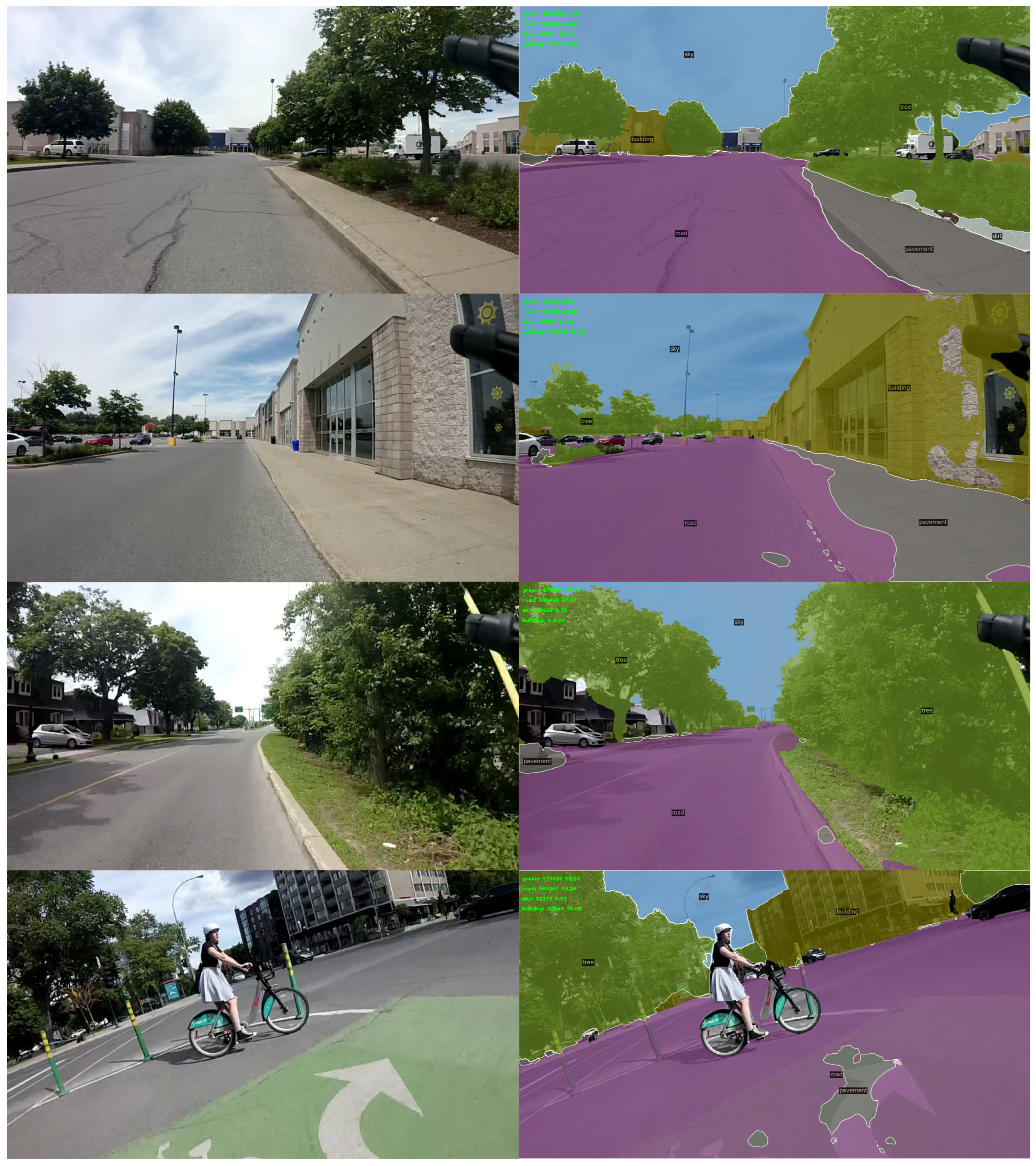
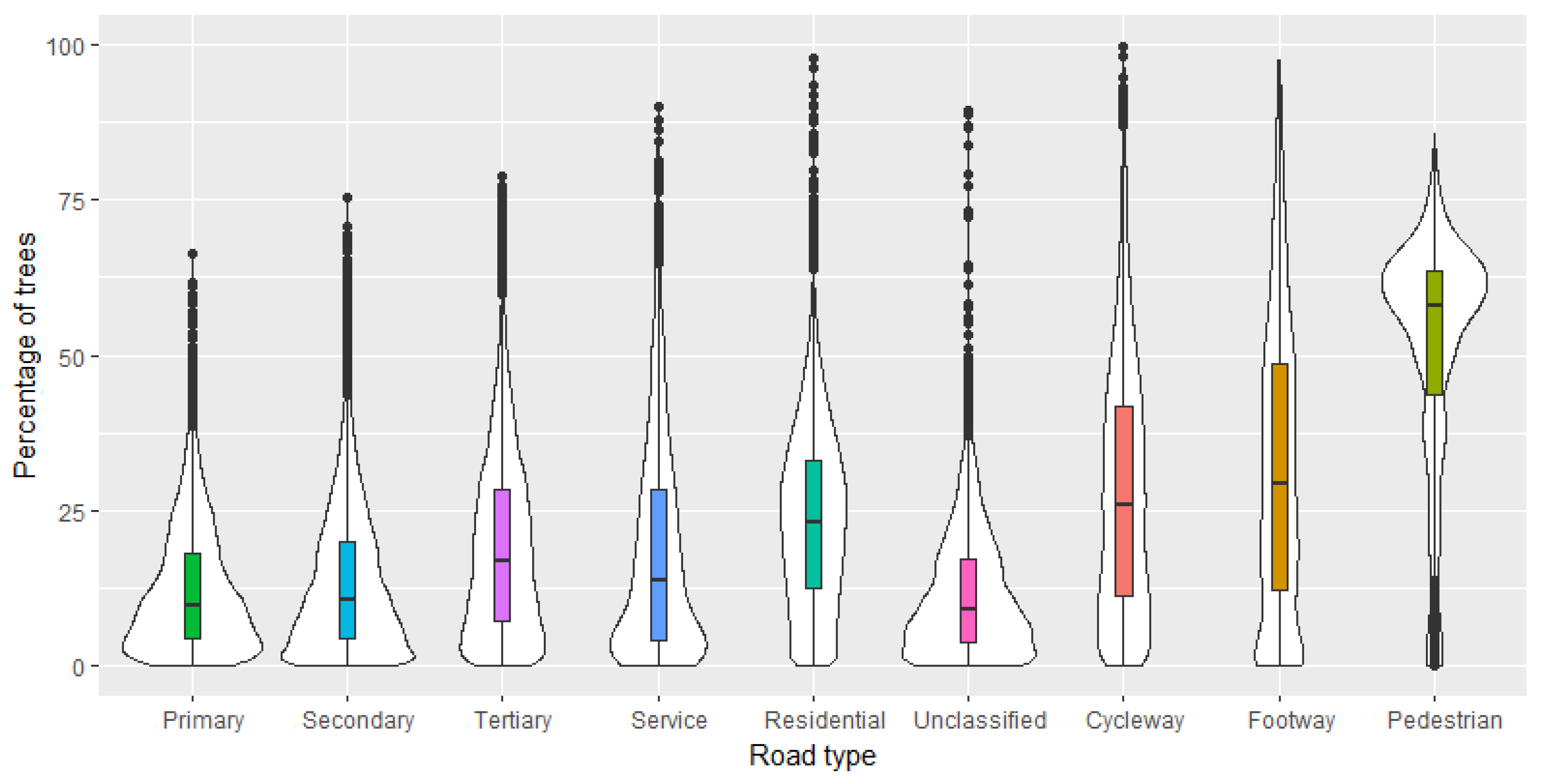
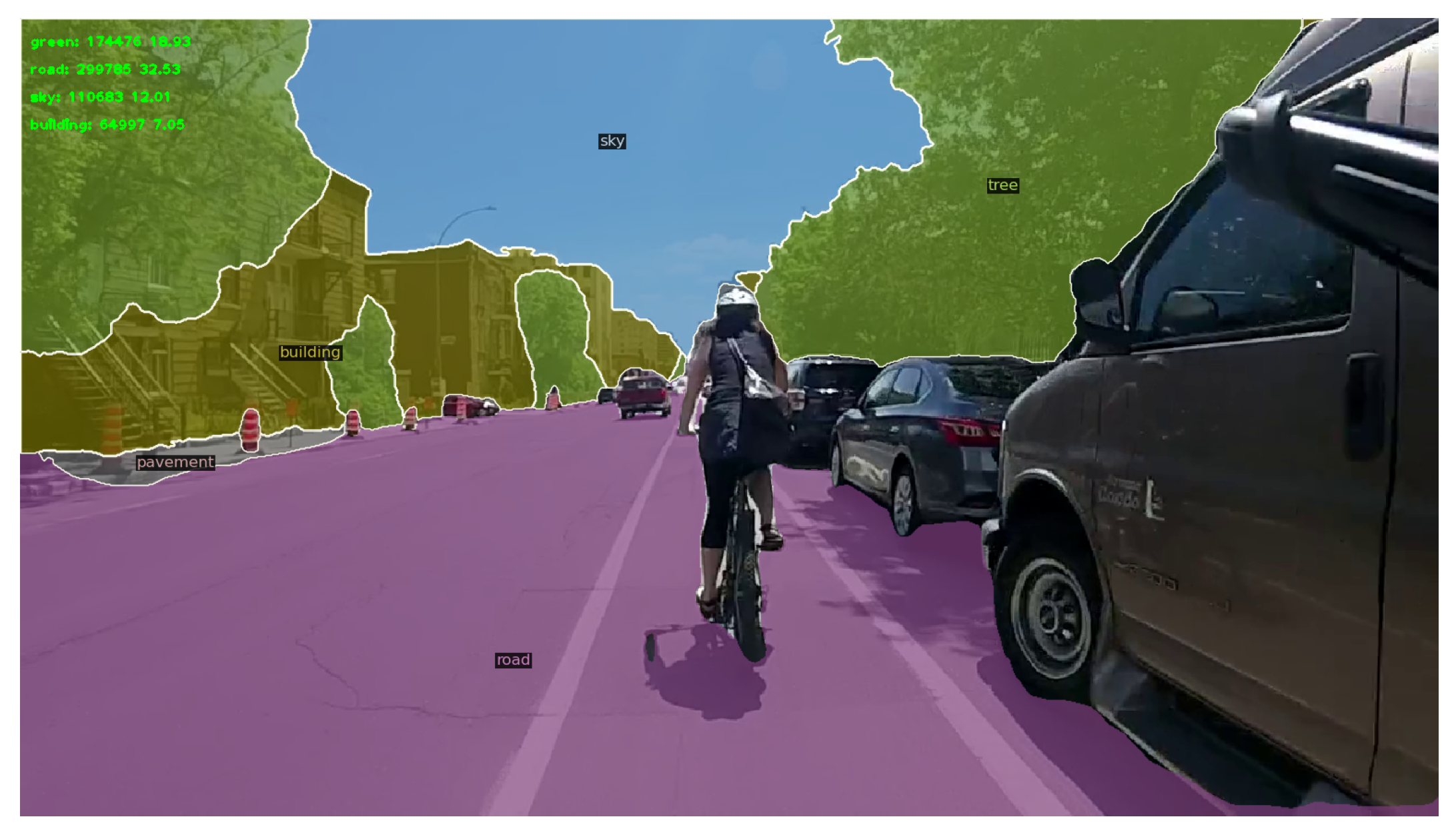
3.1. Tree Detection
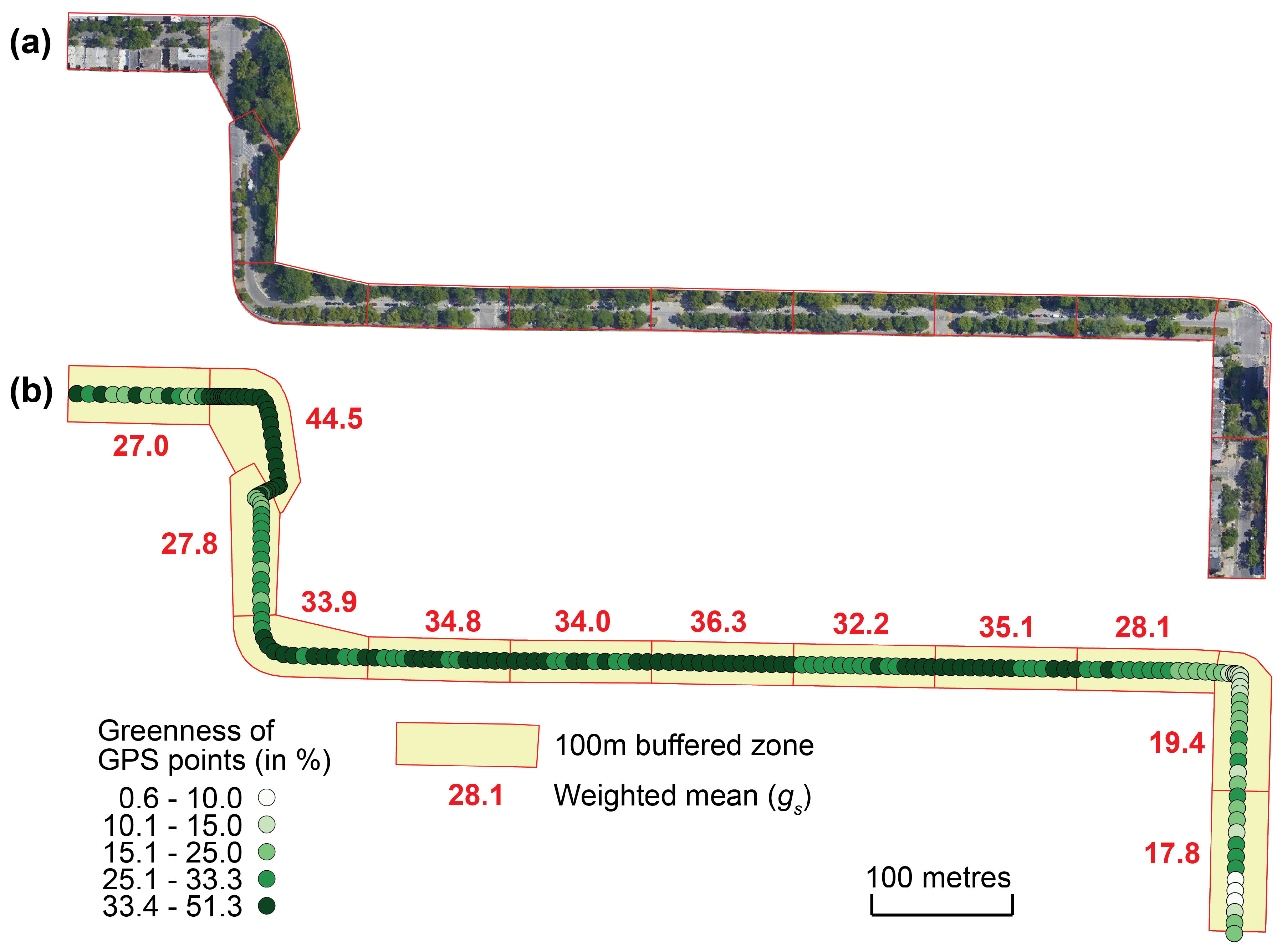
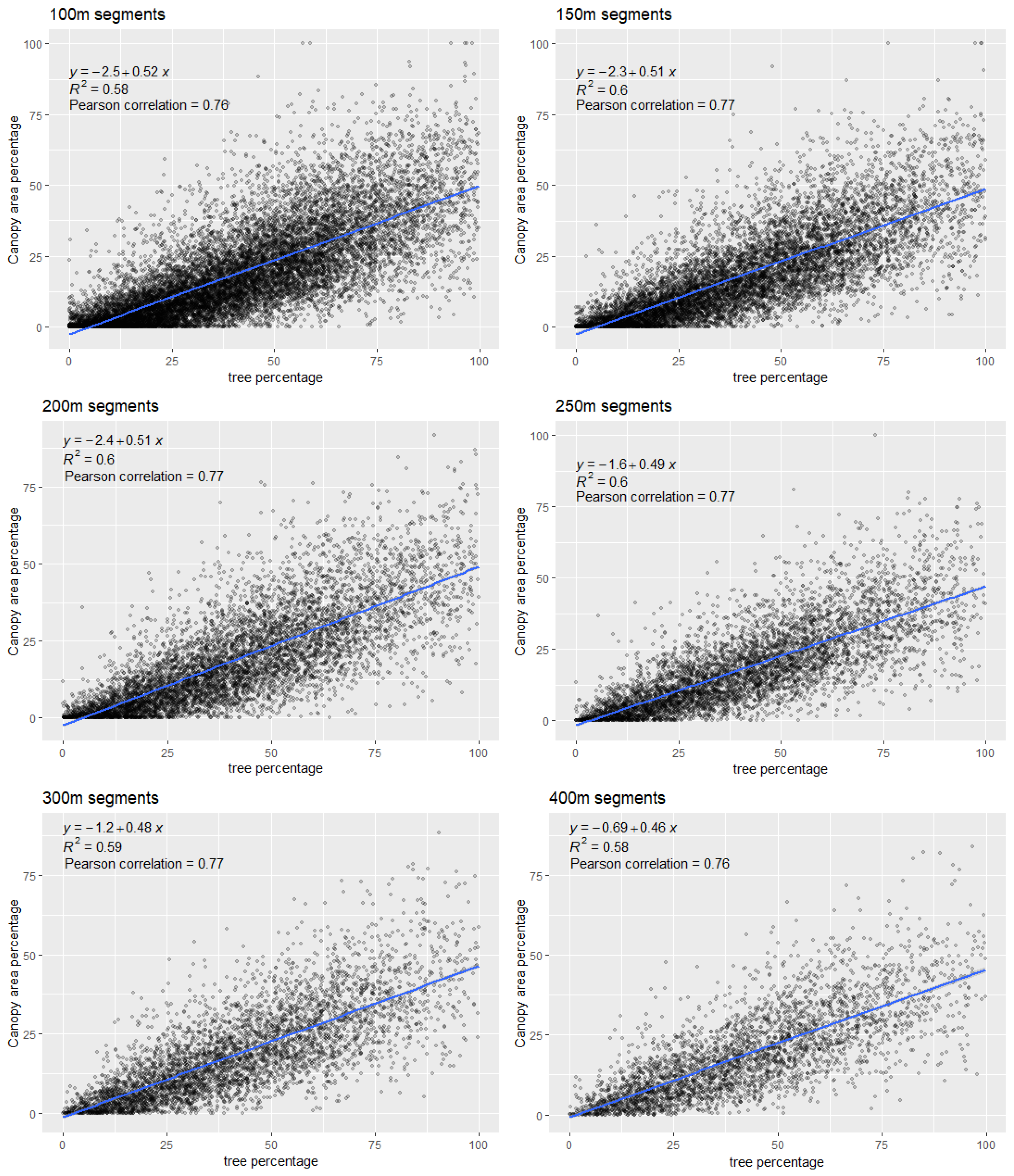
3.2. Correlation between Detected Greenness and Canopy Data
4. Discussion
4.1. Using Detectron2 to Detect Greenness
4.2. Comparing Canopy Data to Video Greenness
5. Conclusions
Author Contributions
Funding
Institutional Review Board Statement
Informed Consent Statement
Data Availability Statement
Acknowledgments
Conflicts of Interest
References
- Bratman, G.N.; Anderson, C.B.; Berman, M.G.; Cochran, B.; de Vries, S.; Flanders, J.; Folke, C.; Frumkin, H.; Gross, J.J.; Hartig, T.; et al. Nature and mental health: An ecosystem service perspective. Sci. Adv. 2019, 5, eaax0903. [Google Scholar] [CrossRef] [PubMed]
- Coventry, P.A.; Brown, J.E.; Pervin, J.; Brabyn, S.; Pateman, R.; Breedvelt, J.; Gilbody, S.; Stancliffe, R.; McEachan, R.; White, P.L. Nature-based outdoor activities for mental and physical health: Systematic review and meta-analysis. SSM-Popul. Health 2021, 16, 100934. [Google Scholar] [CrossRef] [PubMed]
- Bowler, D.E.; Buyung-Ali, L.M.; Knight, T.M.; Pullin, A.S. A systematic review of evidence for the added benefits to health of exposure to natural environments. BMC Public Health 2010, 10, 456. [Google Scholar] [CrossRef]
- Group, B.M.J.P. The health risks and benefits of cycling in urban environments compared with car use: Health impact assessment study. BMJ 2011, 343, d5306. [Google Scholar] [CrossRef]
- Majumdar, B.B.; Mitra, S.; Pareekh, P. On identification and prioritization of motivators and deterrents of bicycling. Transp. Lett. 2020, 12, 591–603. [Google Scholar] [CrossRef]
- Cervero, R.; Caldwell, B.; Cuellar, J. Bike-and-ride: Build it and they will come. J. Public Transp. 2013, 16, 5. [Google Scholar] [CrossRef]
- Winters, M.; Brauer, M.; Setton, E.M.; Teschke, K. Built environment influences on healthy transportation choices: Bicycling versus driving. J. Urban Health 2010, 87, 969–993. [Google Scholar] [CrossRef]
- Stefansdottir, H. A theoretical perspective on how bicycle commuters might experience aesthetic features of urban space. J. Urban Des. 2014, 19, 496–510. [Google Scholar] [CrossRef]
- Parsons, R.; Tassinary, L.G.; Ulrich, R.S.; Hebl, M.R.; Grossman-Alexander, M. The view from the road: Implications for stress recovery and immunization. J. Environ. Psychol. 1998, 18, 113–140. [Google Scholar] [CrossRef]
- Lusk, A.C.; Da Silva Filho, D.F.; Dobbert, L. Pedestrian and cyclist preferences for tree locations by sidewalks and cycle tracks and associated benefits: Worldwide implications from a study in Boston, MA. Cities 2020, 106, 102111. [Google Scholar] [CrossRef]
- Reid, C.E.; Kubzansky, L.D.; Li, J.; Shmool, J.L.; Clougherty, J.E. It’s not easy assessing greenness: A comparison of NDVI datasets and neighborhood types and their associations with self-rated health in New York City. Health Place 2018, 54, 92–101. [Google Scholar] [CrossRef] [PubMed]
- Rhew, I.C.; Vander Stoep, A.; Kearney, A.; Smith, N.L.; Dunbar, M.D. Validation of the Normalized Difference Vegetation Index as a measure of neighborhood greenness. Ann. Epidemiol. 2011, 21, 946–952. [Google Scholar] [CrossRef] [PubMed]
- Lu, Y.; Yang, Y.; Sun, G.; Gou, Z. Associations between overhead-view and eye-level urban greenness and cycling behaviors. Cities 2019, 88, 10–18. [Google Scholar] [CrossRef]
- Li, X.; Zhang, C.; Li, W.; Ricard, R.; Meng, Q.; Zhang, W. Assessing street-level urban greenery using Google Street View and a modified green view index. Urban For. Urban Green. 2015, 14, 675–685. [Google Scholar] [CrossRef]
- Villeneuve, P.J.; Ysseldyk, R.L.; Root, A.; Ambrose, S.; DiMuzio, J.; Kumar, N.; Shehata, M.; Xi, M.; Seed, E.; Li, X.; et al. Comparing the Normalized Difference Vegetation Index with the Google Street View measure of vegetation to assess associations between greenness, walkability, recreational physical activity, and health in Ottawa, Canada. Int. J. Environ. Res. Public Health 2018, 15, 1719. [Google Scholar] [CrossRef]
- Gao, F.; Li, S.; Tan, Z.; Zhang, X.; Lai, Z.; Tan, Z. How is urban greenness spatially associated with dockless bike sharing usage on weekdays, weekends, and holidays? ISPRS Int. J. Geo-Inf. 2021, 10, 238. [Google Scholar] [CrossRef]
- Garrett, B.L. Videographic geographies: Using digital video for geographic research. Prog. Hum. Geogr. 2011, 35, 521–541. [Google Scholar] [CrossRef]
- Büscher, M.; Urry, J. Mobile methods and the empirical. Eur. J. Soc. Theory 2009, 12, 99–116. [Google Scholar] [CrossRef]
- Henao, A.; Apparicio, P. Dangerous overtaking of cyclists in Montréal. Safety 2022, 8, 16. [Google Scholar] [CrossRef]
- Jarry, V.; Apparicio, P. Ride in peace: How cycling infrastructure types affect traffic conflict occurrence in Montréal, Canada. Safety 2021, 7, 63. [Google Scholar] [CrossRef]
- Ismail, K.; Sayed, T.; Saunier, N.; Lim, C. Automated analysis of pedestrian–vehicle conflicts using video data. Transp. Res. Rec. 2009, 2140, 44–54. [Google Scholar] [CrossRef]
- Jackson, S.; Miranda-Moreno, L.F.; St-Aubin, P.; Saunier, N. Flexible, mobile video camera system and open source video analysis software for road safety and behavioral analysis. Transp. Res. Rec. 2013, 2365, 90–98. [Google Scholar] [CrossRef]
- Saunier, N.; Sayed, T. Automated analysis of road safety with video data. Transp. Res. Rec. 2007, 2019, 57–64. [Google Scholar] [CrossRef]
- Jabir, B.; Noureddine, F.; Rahmani, K. Accuracy and efficiency comparison of object detection open-source models. Int. J. Online Biomed. Eng. (iJOE) 2021, 17, 165. [Google Scholar] [CrossRef]
- Mandal, V.; Adu-Gyamfi, Y. Object detection and tracking algorithms for vehicle counting: A comparative analysis. J. Big Data Anal. Transp. 2020, 2, 251–261. [Google Scholar] [CrossRef]
- Winters, M.; Davidson, G.; Kao, D.; Teschke, K. Motivators and deterrents of bicycling: Comparing influences on decisions to ride. Transportation 2011, 38, 153–168. [Google Scholar] [CrossRef]
- Mertens, L.; Van Dyck, D.; Ghekiere, A.; De Bourdeaudhuij, I.; Deforche, B.; Van de Weghe, N.; Van Cauwenberg, J. Which environmental factors most strongly influence a street’s appeal for bicycle transport among adults? A conjoint study using manipulated photographs. Int. J. Health Geogr. 2016, 15, 31. [Google Scholar] [CrossRef]
- Wang, R.; Lu, Y.; Wu, X.; Liu, Y.; Yao, Y. Relationship between eye-level greenness and cycling frequency around metro stations in Shenzhen, China: A big data approach. Sustain. Cities Soc. 2020, 59, 102201. [Google Scholar] [CrossRef]
- OpenStreetMap Contributors. Planet Dump Retrieved. 2017. Available online: https://planet.osm.org (accessed on 26 December 2022).
- OpenStreetMap. Key:highway. 2022. Available online: https://wiki.openstreetmap.org/wiki/Key:highway (accessed on 26 December 2022).
- Communauté métropolitaine de Montréal, Données géoréférencées de l’Observatoire du Grand Montréal: Indice de canopée métropolitain. 2022. Available online: https://observatoire.cmm.qc.ca/produits/donnees-georeferencees/#indice_canopee (accessed on 26 December 2022).
- Bradski, G. The openCV library. Dr. Dobb’s J. Softw. Tools Prof. Program. 2000, 25, 120–123. [Google Scholar]
- Wu, Y.; Kirillov, A.; Massa, F.; Lo, W.Y.; Girshick, R. Detectron2. 2019. Available online: https://github.com/facebookresearch/detectron2 (accessed on 26 December 2022).
- Paszke, A.; Gross, S.; Massa, F.; Lerer, A.; Bradbury, J.; Chanan, G.; Killeen, T.; Lin, Z.; Gimelshein, N.; Antiga, L.; et al. PyTorch: An imperative style, high-performance deep learning library. In Advances in Neural Information Processing Systems 32; Wallach, H., Larochelle, H., Beygelzimer, A., d’Alché-Buc, F., Fox, E., Garnett, R., Eds.; Curran Associates, Inc.: Red Hook, NY, USA, 2019; pp. 8024–8035. [Google Scholar]
- Lin, T.Y.; Maire, M.; Belongie, S.; Bourdev, L.; Girshick, R.; Hays, J.; Perona, P.; Ramanan, D.; Zitnick, C.L.; Dollár, P. Microsoft COCO: Common objects in context. arXiv 2015, arXiv:1405.0312. [Google Scholar] [CrossRef]
- Jordahl, K.; Bossche, J.V.d.; Fleischmann, M.; Wasserman, J.; McBride, J.; Gerard, J.; Tratner, J.; Perry, M.; Badaracco, A.G.; Farmer, C.; et al. geopandas/geopandas: V0.8.1. Zenodo. 2020. [Google Scholar] [CrossRef]
- R Core Team. R: A Language and Environment for Statistical Computing; R Foundation for Statistical Computing: Vienna, Austria, 2021. [Google Scholar]
- QGIS Development Team. QGIS Geographic Information System. 2022. Available online: https://www.qgis.org (accessed on 26 December 2022).


| Type of Road 1 | N | % | HH:MM:SS |
|---|---|---|---|
| Primary | 14,650 | 4.70 | 04:04:10 |
| Secondary | 70,968 | 22.79 | 09:42:48 |
| Tertiary | 69,996 | 22.47 | 19:26:36 |
| Service | 2233 | 0.72 | 00:37:13 |
| Residential | 96,636 | 31.03 | 26:50:36 |
| Unclassified | 5938 | 1.91 | 01:38:58 |
| Cycleway | 40,587 | 13.03 | 11:16:27 |
| Footway | 8765 | 2.81 | 02:26:05 |
| Pedestrian | 1673 | 0.54 | 00:27:53 |
| Total | 311,446 | 100.0 | 86:30:46 |
| Tree | Road | Sky | Building | |
|---|---|---|---|---|
| Percentiles | ||||
| 1 | 0.0 | 0.5 | 0.0 | 0.0 |
| 5 | 0.8 | 10.6 | 1.5 | 0.0 |
| 10 | 2.3 | 18.0 | 3.2 | 0.0 |
| 25 | 7.3 | 28.6 | 8.1 | 0.0 |
| 50 | 17.5 | 39.3 | 16.3 | 2.7 |
| 75 | 29.9 | 48.0 | 26.7 | 11.2 |
| 90 | 41.8 | 55.3 | 36.9 | 22.9 |
| 95 | 49.4 | 58.9 | 42.9 | 30.1 |
| 99 | 65.8 | 65.6 | 54.2 | 42.4 |
| Mean | 20.2 | 37.8 | 18.5 | 7.5 |
| SD 1 | 15.7 | 14.4 | 13.0 | 10.3 |
| Segment Length | 100 m | 150 m | 200 m | 250 m | 300 m | 400 m |
|---|---|---|---|---|---|---|
| n 1 | 13,978 | 9309 | 6972 | 5569 | 4625 | 3444 |
| Percentiles | ||||||
| 1 | 0.0 | 0.0 | 0.0 | 0.0 | 0.0 | 0.0 |
| 5 | 0.0 | 0.0 | 0.1 | 0.2 | 0.4 | 0.8 |
| 10 | 0.2 | 0.7 | 1.1 | 1.7 | 1.7 | 2.2 |
| 25 | 4.2 | 5.1 | 5.5 | 6.6 | 6.6 | 7.0 |
| 50 | 14.5 | 15.0 | 15.3 | 15.9 | 15.9 | 16.3 |
| 75 | 29.6 | 28.9 | 28.9 | 28.6 | 28.6 | 28.0 |
| 90 | 46.7 | 45.3 | 43.6 | 42.6 | 42.0 | 40.8 |
| 95 | 57.4 | 55.5 | 53.6 | 52.8 | 51.6 | 49.4 |
| 99 | 82.9 | 77.8 | 77.5 | 76.3 | 73.5 | 72.3 |
| Mean | 19.6 | 19.6 | 19.6 | 19.6 | 19.6 | 19.5 |
| SD 2 | 19.1 | 18.2 | 17.6 | 17.2 | 16.7 | 16.2 |
| Tree | Road | Sky | Building | |
|---|---|---|---|---|
| Tree | ||||
| Road | 0.113 | |||
| Sky | ||||
| Building | 0.113 |
Disclaimer/Publisher’s Note: The statements, opinions and data contained in all publications are solely those of the individual author(s) and contributor(s) and not of MDPI and/or the editor(s). MDPI and/or the editor(s) disclaim responsibility for any injury to people or property resulting from any ideas, methods, instructions or products referred to in the content. |
© 2022 by the authors. Licensee MDPI, Basel, Switzerland. This article is an open access article distributed under the terms and conditions of the Creative Commons Attribution (CC BY) license (https://creativecommons.org/licenses/by/4.0/).
Share and Cite
Bourassa, A.; Apparicio, P.; Gelb, J.; Boisjoly, G. Canopy Assessment of Cycling Routes: Comparison of Videos from a Bicycle-Mounted Camera and GPS and Satellite Imagery. ISPRS Int. J. Geo-Inf. 2023, 12, 6. https://doi.org/10.3390/ijgi12010006
Bourassa A, Apparicio P, Gelb J, Boisjoly G. Canopy Assessment of Cycling Routes: Comparison of Videos from a Bicycle-Mounted Camera and GPS and Satellite Imagery. ISPRS International Journal of Geo-Information. 2023; 12(1):6. https://doi.org/10.3390/ijgi12010006
Chicago/Turabian StyleBourassa, Albert, Philippe Apparicio, Jérémy Gelb, and Geneviève Boisjoly. 2023. "Canopy Assessment of Cycling Routes: Comparison of Videos from a Bicycle-Mounted Camera and GPS and Satellite Imagery" ISPRS International Journal of Geo-Information 12, no. 1: 6. https://doi.org/10.3390/ijgi12010006
APA StyleBourassa, A., Apparicio, P., Gelb, J., & Boisjoly, G. (2023). Canopy Assessment of Cycling Routes: Comparison of Videos from a Bicycle-Mounted Camera and GPS and Satellite Imagery. ISPRS International Journal of Geo-Information, 12(1), 6. https://doi.org/10.3390/ijgi12010006