Abstract
Numerous autonomous robots are used not only for factory automation as labor saving devices, but also for interaction and communication with humans in our daily life. Although superior compatibility for semantic recognition of generic objects provides wide applications in a practical use, it is still a challenging task to create an extraction method that includes robustness and stability against environmental changes. This paper proposes a novel method of scene and position recognition based on visual landmarks (VLs) used for an autonomous mobile robot in an environment living with humans. The proposed method provides a mask image of human regions using histograms of oriented gradients (HOG). The VL features are described with accelerated KAZE (AKAZE) after extracting conspicuous regions obtained using saliency maps (SMs). The experimentally obtained results using leave-one-out cross validation (LOOCV) revealed that recognition accuracy of high-saliency feature points was higher than that of low-saliency feature points. We created our original benchmark datasets using a mobile robot. The recognition accuracy evaluated using LOOCV reveals 49.9% for our method, which is 3.2 percentage points higher than the accuracy of the comparison method without HOG detectors. The analysis of false recognition using a confusion matrix examines false recognition occurring in neighboring zones. This trend is reduced according to zone separations.
1. Introduction
Numerous autonomous robots have come to be used in the remarkable progress of the robot industry. They are used not only for factory automation as labor saving devices, but also for interaction and communication with humans in our daily life. For these robots having roles and collaboration with humans, it is necessary to obtain capabilities for purposive judgment and autonomous behavior. To locomotion in an actual environment autonomously, robots must avoid collision with humans or objects that are recognized in real time. Moreover, robots must recognize their position to ascertain surroundings, to perform risk prediction, and to formulate return procedures to be used after collision avoidance. Actually, intelligent behavior and functions are actualized through updating of the processes of the obtained information, including a robot’s position in real time because robots autonomously collect diverse information as their environment changes dynamically.
To actualize autonomous robot locomotion, three approaches are posited. The first approach is to use a static map prepared in advance. As a benefit for this approach, it is simple and easy for position estimation and recognition. However, a shortcoming is its vulnerability to environmental changes because it uses fixed map information. The second approach is to use a dynamic map after creation. For this approach, numerous methods have been proposed based on simultaneous localization and mapping (SLAM) [1], which is used for map creation, position estimation, and navigation. A benefit for this approach is its robustness for environmental changes because it uses a dynamic map that is updated in real time. A shortcoming is its high calculation cost for sensing signals obtained from wide-range precision and sensors, such as stereo cameras and laser range finders (LRFs), which are expensive sensing devices used to obtain metric information. The third approach is to use landmarks. Without using a static or dynamic map, this approach is simple and practical. According to landmark types, this approach is divisible into two categories: a preset landmark-based approach and a visual landmark (VL)-based approach, which uses visual saliency objects in a scene. As a benefit of the preset landmark approach, steady landmark extraction and position recognition is actualized because of using landmark features that are already known. A shortcoming is not only the burden of landmark installation in advance, but also its uselessness for a new environment without landmarks. In contrast, the VL-based approach requires no landmark installation in advance before locomotion with providing adaptation in various environments. For this approach, specific and costly sensors are unnecessary because various and diverse generic objects are used as VLs. Similar to human perception, superior compatibility for semantic recognition of generic objects provides wide applications in a practical use. However, it is still a challenging task to create an extraction method that includes robustness and stability against environmental changes.
Although numerous methods that are widely used in indoor environments have been proposed, it is still a challenging task for practical applications. Exit studies were merely evaluated with simulation and a limited environment without environmental changes. Moreover, these are no consideration for human effects or interference in an actual environment with existing humans. Therefore, evaluation experiments were conducted under the hidden assumption that exits steady detected landmarks in an environment. This paper proposes a novel method to achieve automobile locomotion of a human symbiotic robot based on VL extraction and recognition in an actual environment. As basic performance measurements, we evaluated our method using benchmark datasets of two types for semantic scene recognition and human detections. Subsequently, we evaluated the performance of our method using our original benchmark datasets of two types without humans and with humans that were obtained using a mobile robot. This paper presents comparison results of recognition accuracies for scene and positional recognition as localization of autonomous locomotion based on VLs in an actual environment.
The rest of the paper is structured as follows. In Section 2, related studies are presented, especially for approaches based on visual landmarks combine with machine learning algorithms. Section 3 presents our proposed method based on visual saliency and a supervised machine learning approach. Subsequently, Section 4, Section 5 and Section 6 present experimentally obtained results using two benchmark datasets and one original dataset obtained using a monocular camera mounted on a mobile robot. Finally, Section 7 concludes and highlights future work. Herein, we had proposed this basic method in the proceedings [2,3]. For this paper, we have described detail results and discussion in Section 6.
2. Related Studies
Since the 1990s, studies on VL-based position estimation have attracted attention according to the performance progress and cost effectiveness of computers and cameras used for visual sensors [4]. In 2002, Desouza et al. had surveyed numerous studies related to vision for mobile robot navigation in 20 years. They dealt with indoor navigation and outdoor navigation for 165 references. For their categorization, indoor navigation was divided to three approaches: map-based navigation, map-building-based navigation, and map-less navigation. Moreover, they categorized map-less navigation into three approaches: navigation using optical flow-based navigation, navigation using appearance-based matching, and navigation using object recognition. In those days, there were merely two cases for the approach of navigation using object recognition because of insufficient computational capability.
In the early stage of VL detection, edges and corners obtained from objects and background patterns were used as landmark features. Since part-based feature description was introduced into generic object recognition [5], robustness for positions, scales, and rotations of landmarks has improved dramatically. Li et al. propose a method to learn and recognize natural scene categories using Bayesian hierarchical models. The primary feature of their method was to learn characteristic intermediate themes of scenes with no supervision. Although recognition accuracy was inferior to supervised-learning methods, their method did not require experts to annotate training datasets. As a pioneer study for saliency-based object recognition, Shokoufandeha et al. [6] proposed a saliency map graph (SMG) that captured salient regions of an object viewed at multiple scales using a wavelet transform. They defined saliency as informedness, or more concretely, as significant energy responses as computed by filters. For attending objects before recognition, Walther el al. [7] proposed a biologically plausible model to detect proto-objects in natural scenes based on salience maps (SMs) [8]. They described scale-invariant feature transform (SIFT) [9] over attended proto-objects. For complex scene images, they demonstrated clear reduction to match key-points constellation in objet recognition. Nevertheless, no guarantee exists that their region-selection algorithm can find objects. Their method remains purely bottom-up, stimulus driven, with no prior notion of objects in semantics.
As a remarkable study using Graph Based Visual Saliency (BGVS) [10], Kostavelis et al. [11] proposed a bio-inspired model for pattern classification and object recognition. They exploited Hierarchical Temporal Memory (HTM) for comprising a hierarchical tree structure. The experimentally obtained results evaluated using ETH-80 benchmark dataset revealed that their model achieved greater accuracy of pattern classification and object recognition compared with other HTM-based methods. Moreover, Kostavelis et al. [12] introduced a coexistence model of accurate SLAM and place recognition for a descriptive and adaptable navigation used in indoor environments. Their model comprises a novel content-based representation algorithm for spatial abstraction and a bag-of-features method using a Neural Gas for coding the spatial information for each scene. They used support vector machines (SVMs) as a classifier that actualized accurate recognition of multiple dissimilar places. The experimentally obtained results evaluated using several popular benchmark datasets reveled that their proposed method achieved remarkable accuracy. Moreover, their proposed method produced semantic inferences suitable for labeling unexplored environments. Based on their excellent studies, they [13] surveyed semantic mapping techniques including publicly available validation datasets and benchmarking with addressing issues and questions. Actually, semantics in robotics is very well known procedure. However, our study is not included in semantics, merely using VLs.
According to the remarkable computational progress in recent years, numerous methods have been proposed for VL-based semantic position recognition. Chen et al. [14] developed a simple and cost-effective position identification system using augmented reality (AR) markers that were installed on a ceiling in advance. Although they described a practical application used for a navigation task, their evaluation remained merely computer simulation without evaluation results obtained using an actual mobile robot. Chang et al. [15] proposed a fusion method of Gist and SMs [8] for robotic tracking based on template matching among saliency features. They evaluated their method in a 37-m-long indoor environment and a 138-m-long outdoor environment. However, the Gist representation performance was insufficient for indoor scenes as a global feature descriptor in natural scenes with large-scale structures. Moreover, the problem of template matching remained to improve the calculation cost and noise tolerance. Hayet et al. [16] proposed a landmark recognition method using Harris operators and partial Hausdorff distance combined with extracting landmark candidates searched for edge features and rectangular regions. The limitation of their method was in landmark extraction because of relaying edges for feature description. Sala et al. [17] proposed a graph theory as heuristic algorithm for selecting suitable landmark combination using SIFT [9]. Although they described SIFT features from whole images, the evaluation results showed insufficient capability for environmental changes because of limited evaluation for robustness.
Hayet et al. [18] proposed a sensor fusion system using an LRF, which is used for environmental modeling with a generalized Voronoi graph (GVG), and a monocular camera, which is used for a framework of landmark learning and recognition. The experimentally obtained results remained merely graph model creation using GVG at a corridor with no numerical evaluation results. Se et al. [19] proposed a SIFT-based scale-invalid VLs extraction method with tracking them using a Kalman filter applied in a dynamic environment. For applying a dynamic environment changed objects in real-time, Se et al. [19] proposed a VL tracking method using a Kalman filter combined with extracting scale-invalid VLs using SIFT features. They measured the degree of uncertainty for detected landmarks to approximate an ellipse. However, no matching results were provided for position identification. Livatino et al. [20] proposed a method to extract salient regions using four features: edges, corners, luminance, and local symmetry. They set VLs as doorknobs, posters, and power switch buttons. The experimentally obtained results revealed that they evaluated their method merely for a limited environment without sufficient generalization. Accuracies of existing methods for position estimation and navigation were evaluated under the assumption of steady VL extraction. They provided no consideration of occlusion and corruption of objects as VLs. The primary concern of the existing studies was highly accurate object detection without consideration of occlusion by human effects.
For human-symbolic robots, it is necessary to evaluate robustness for human interference that is unavoidable in actual environments. Bestgen et al. [21] examined a conceptual model for automatisms of navigation using volunteered geographic information (VGI)-based landmarks. Their model includes a concept that systematic cognitive aspects of humans and their interests. Based on selected landmarks and patterns of landmarks building geometric shapes, they expected guidance of spatial attention and support individual way finding strategies. We consider that it is worth considering aspects of spatial cognition in humans including a systematic impact on robot behavior. Morioka et al. [22] proposed a local map creation and navigation method used for an indoor mobile robot in a dynamic and crowded environment with humans. To extract time-series features for matching, they proposed a novel descriptor named position invariant robust features (PIRFs) based on SIFT. They actualized real-time navigation combined with 3D-map creation using PIRFs for extracting metric information from time-series images. Noguchi et al. [23] proposed a mobile path creation method using human trajectories. For learning trajectories, they actualized human behavior prediction and path planning for avoiding human interference. Their method calculated a human behavior probability map to update path planning tables in real time. For human mobility measurement, they used LRFs fixed in an environment and particle filters to track human positions. However, evaluation experiments were merely conducted in computer simulations. Although several methods were presented for reducing human effect, no method has been proposed for autonomous VL-based locomotion.
3. Proposed Method
3.1. Entire Procedure
We specifically examine the effect human interference in scene recognition using visual information. Figure 1 depicts the whole procedure of our proposed method for detecting, extracting, and describing VLs. Our method comprises saliency region detection using SMs [8], feature description using accelerated KAZE (AKAZE) [24], and human detection with masking using a histogram of oriented gradients (HOG) [25]. Using SMs, regions with high saliency can be extracted as VL candidates. Human regions, which are excluded with HOG masking in images, are excluded with HOG masking. Our method extracts AKAZE features from this region. Intersection areas between SMs and HOG masks are used for candidate areas as VLs after extracting AKAZE features.
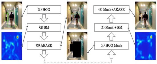
Figure 1.
Whole procedure of our proposed method that comprises saliency region detection using SMs, feature description using AKAZE, and human detection with masking using a HOG.
Let , , and be an original image, a SM binary mask image, and a HOG mask image. The output image is defined as the following.
For scene recognition, we used adaptive category mapping networks (ACMNs) [26] that learn adaptively, along with additional sequential signal features with visualization of topological relational structures as a category map (CM). ACMNs comprise three modules: a codebook module, a labeling module, and a mapping module. As shown in Figure 2, we used the codebook module for quantizing input signals using self-organization maps (SOMs) [27] and the mapping module for visualizing spatial relations among input signals as a CM using counter propagation networks (CPNs) [28]. For this study, we did not use the labeling module, which comprises adaptive resonance theory (ART) [29] networks, because we solely used the supervised learning mode.
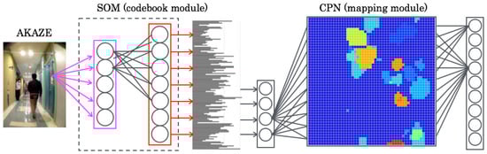
Figure 2.
Codebook module for quantizing input signals using SOMs and mapping module for visualizing spatial relations among input signals.
3.2. Feature Signal Description
Gist [30] is a descriptor used to extract features from outdoor images, especially for global scene structures such as rivers, mountains, lakes, forests, and clouds in nature. Because of its rough description granularity, it is unsuitable for describing features of indoor scenes and objects as our target objects. As a part-based feature descriptor, SIFT [9] is used popularly and widely in computer vision studies and numerous applications, especially for generic object description and recognition. Using nonlinear scale spaces, KAZE descriptors [31] recorded superior performance than SIFT descriptors did. As an improved model, AKAZE descriptors [24] are especially examined for excellent descriptive capability and low processing costs as real-time image processing.
3.3. Saliency Map
Let be an intensity channel defined as
where r, g, and b respectively represent red, green, and blue channels. The hue channel comprises RGB and the yellow channel , which is calculated as
Orientation channels are created on the edge of four directions: = 0, 45, 90, and 135 degree. Gabor filter is defined as the product of the sine wave and the Gaussian function. is defined as shown below.
Therein, , , , and respectively represent the wavelength of the cosine component, the direction component of the Gabor function, the filter size in the vertical axis direction, and the filter size in the horizontal axis direction. The integral value to the vertical axis is the maximum if G is applied to lines with gradients in the image. We extract the gradient and frequency components using the above property. The filter size is defined as pixels. The filter output at the sample point is defined as
where Z is a complex term as .
The attention positions are identified by superimposing the differences among different scale pairs, which are obtained from images using Gaussian pyramid. These are designated as center–surround operations, which are represented by the operator ⊖. For the difference operation, small images are extended to large images. When defining scales as c, s (), a larger scale is represented as ; a smaller one is represented as . For the intensity component, the difference is calculated as shown below.
Let and respectively represent the differences between the red and green component and the blue and yellow component.
Orientation features are obtained from the difference in each direction.
After normalizing, feature maps (FMs) are superimposed in each channel. Herein, small maps are zoomed for summation in each pixel. Let N be a normalization function. Linear summations of intensity channel , color channel , and orientation channel are defined as the following.
The obtained maps are referred for conspicuity maps. Normalizing respective channels of FMs and linear summation, SMs are obtained as
Finally, high saliency regions are extracted using winner-take-all (WTA) competition [32].
3.4. Codebooks
Let and respectively denote input data and weights from an input layer unit i to a mapping layer unit j at time t. Herein, I and J respectively denote the total numbers of the input layer and the mapping layer. Before learning, are initialized randomly. The unit for which the Euclidean distance between and is the smallest is sought as the winner unit of its index as
As a local region for updating weights, the neighborhood region is defined as the center of the winner unit as
Therein, is the initial size inside ; O is the maximum iteration for training; and coefficient 0.5 is appended as a floor function for rounding.
Subsequently, in are updated to close input feature patterns as
Therein, is a learning coefficient that decreases concomitantly according to the learning progress.
3.5. Recognition
Let be weights from an input layer unit i to a Kohonen layer unit at time t. Therein, are weights from a Grossberg layer unit j to a Kohonen layer unit at time t. These weights are initialized randomly. Training data show input layer units i at time t. The unit for which the Euclidean distance between and is the smallest is sought as the winner unit of its index as
Here, as in Equation (16), N is a neighborhood region around winner unit . In addition, and inside N are updated respectively by Kohonen’s algorithms and Grossberg’s algorithms as shown below.
Therein, is a teaching signal that is supplied from the Grossberg layer. Furthermore, and are the learning coefficients that decrease concomitantly with learning progress. The CPN learning repeats up to the learning iteration that was set in advance.
4. Preliminary Experiment Using Benchmark Datasets without Humans
4.1. Dataset Details
We used the open benchmark dataset KTH-IDOL2 [33] which is a widely used dataset for vision-based indoor robot navigation and position estimation. Time-series images with 320 × 240 pixel resolution were obtained separately in various environmental setups by two mobile robots. For this study, we used the benchmark dataset obtained using the higher robot after downsampling images from 30 fps to 10 fps with linear interpolation. For the datasets, local positional annotations are contained as ground truth (GT) compared with latest datasets such as MIT Places2 [34] Our recognition target categories comprises the printer area (PA), one-person office (BO), two-person office (EO), kitchen (KT), and corridor (CR) according to the GT signals. We used 12 datasets obtained in three illumination and weather conditions: sunny, cloudy, and night.
4.2. Parameters and Evaluation Criteria
Table 1 presents parameters of SOMs and CPNs that were set based on our earlier study [26]. As our experiment in advance, we verified that the parameter dependence was slight. For evaluation criteria, recognition accuracy for a test dataset is defined as
where and respectively represent the total numbers of test images and GT images. We used leave-one-out cross-validation (LOOCV) [35] for evaluating results along with machine-learning and evolutional-learning approaches.

Table 1.
Optimized parameters used for this preliminary experiment.
4.3. Feature Extraction Results
Figure 3 depicts feature extraction results of AKAZE descriptors and SMs for three example images in KT. The third and fourth rows respectively show images of and as feature points in high-saliency and low-saliency regions surrounded by the red non-linear lines. Although the illumination effect is slight in this environment, the distribution of AKAZE features differs in each image. For perspective analyzing, numerous feature points are distributed in the trash box, the broom, the picture, the doorway frames, and the backside door. Although these images were taken in KT, the features from other rooms are included with illumination changes. The high-saliency regions in night images are different from those in the sunny or cloudy images.
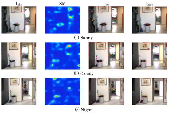
Figure 3.
Feature extraction results in KT.
Figure 4 depicts feature extraction results in CR of which sunlight entered from the glass door in sunny weather conditions. During the time that the datasets were obtained, the lights were turned off that provided the wide contrast gap between the center and the surrounding of respective images. In cloudy and night condition images, the lights were turned on that provided visible of objects such as a partition and posters. Compared with KT images, SM regions are completely different among the three illumination conditions.
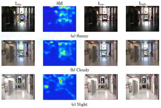
Figure 4.
Feature extraction results in CR.
4.4. Comparison Results
Figure 5, Figure 6 and Figure 7 respectively depict in each scene categories of different weather and illumination conditions: sunny, cloudy, and night. In sunny conditions, of is 0.5 percentage points higher than that of Subsequently, of is 1.7 percentage points higher than that of in cloudy conditions. However, of is 0.4 percentage points lower than that of in night conditions. In respective scene categories, CR gave lower accuracy for .
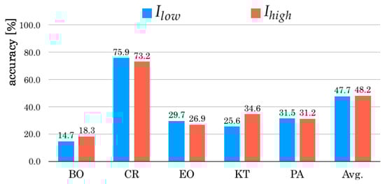
Figure 5.
Comparison results of in respective sunny conditions.
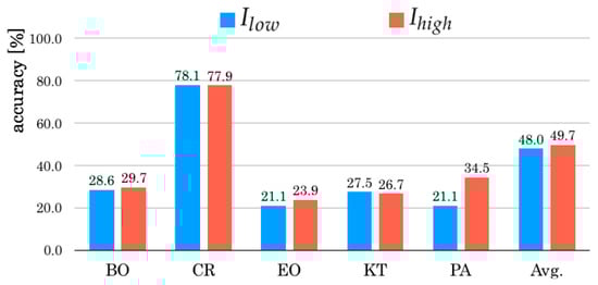
Figure 6.
Comparison results of in respective cloudy conditions.
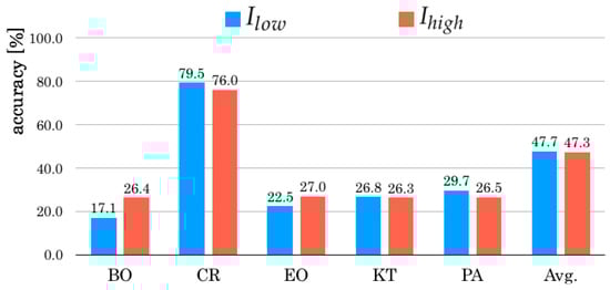
Figure 7.
Comparison results of in respective night conditions.
4.5. Confusion Matrix Analysis
We analyzed false recognition scene images using a confusion matrix. For this matrix, the number of correct recognition images is depicted in the diagonal cells marked with bold text. The underlined values represent the maximum numbers of false recognition images in respective scenes. As the basis for the horizontal cells, the numbers of false recognition images and their labels are specified to the referred labels on the vertical cells. In this dataset, doors physically separate all rooms, including CR. However, as one exception, PA is a continuation of CR which is treated as a separate room because of its different functionality [33]. Therefore, the recognition between PA and CR produce numerous errors.
Table 2, Table 3 and Table 4 correspond to the confusion matrixes in sunny, cloudy, and night conditions, respectively. These matrixes correspond to Figure 5, Figure 6 and Figure 7. The accuracies obtained for BO are the lowest among them. Although BO and EO included similar features due to an office room, numerous images were falsely recognized to KT and CR. The false recognition images in EO showed a similar trend in BO. The number of false recognition images to CR is higher compared with those of the other scene categories.
Table 2.
Confusion matrixes in sunny conditions.
Table 3.
Confusion matrixes in cloudy conditions.
Table 4.
Confusion matrixes in night conditions.
The computational processing time of our method was approximately 3 s per image that depends on the number of AKAZE feature points. The calculation burden was slight in the test mode of SOMs and CPNs. As our former study, we implemented back-propagation neural networks on field-programmable gate arrays (FPGAs) [36]. We consider that we can actualize real-time video processing used for robot vision applications if we use the FPGA implementation technology of part-based feature descriptions [37].
5. Human Detection Experiment
5.1. Dataset Details
As a preliminary step prior to basic performance evaluation of HOG-based human detection, we used EPFL benchmark dataset [38]. This dataset is provided by the Computer Vision Laboratory, School of Computer and Communication Sciences, Swiss Federal Institute of Technology in Lausanne. The video sequence images of EPFL dataset were obtained using multiple cameras installed 2 m above from the ground. For this evaluation experiment, we selected image from four scene categories: Laboratory, Terraces 1 and 2, and Passageway. After converting video images to static images in 1 fps, we used 100 randomly selected images for the evaluation of human detection accuracies.
5.2. Evaluation Criteria
As evaluation criteria, we used the true positive rate (TPR), which is defined using true positive (TP) images and false positive (FP) images as
TPR is moreover regarded as primary as the aim to identify all real positive cases [39]. Moreover, we used the false negative rate (FNR), which is defined using TP images and false negative (FN) images as
FNR is the proportion of real positives that are predicted negatives [39]. As an exception, TP and FP are increased, respectively, to 1 and if n detection windows are overlapped onto a detected human. Similarly, TP and FN are increased, respectively, to 1 and if a detection window contains n detected humans.
5.3. Experimental Results
Figure 8 depicts sample images of human detection results. The green colored rectangles demonstrate HOG regions in four scene categories. Table 5 presents TPR and FNR in each scene category. The mean TPR and FNR for all images were, respectively, 85.4% and 41.6%. The FNR tended to be higher, especially in Terrace 2, which recorded the highest TPR and the second highest FNR next to Passageway. The TPR in Laboratory was 88.8%, which has the lowest FNR and the second lowest of TPR next to Passageway. The TPR and FNR in Passageway were, respectively, the lowest and the highest among four scene categories. This gap means detection difficulty because of the long-depth space and small shaped pedestrians at the scenes. In contrast, the both evaluation criteria showed subordinated relations according to statistical features as an overall trend.
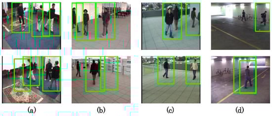
Figure 8.
Human detection results: (a) Laboratory, (b) Terrace 1, (c) Terrace 2, and (d) Passageway.
Table 5.
Accuracies of human detection.
Herein, HOG has no invariant property for scale changes because graduated features are calculated from fixed-size windows. Images tend to be easily recognized if pedestrians are sufficiently large or close to a camera. In contrast, TN is increased if the pedestrians are relatively small or far from a camera with low resolution. Moreover, TN occurred numerously in occlusion or corruption of more than 50% that included for this benchmark dataset.
6. Evaluation Experiment Using Benchmark Datasets Humans
6.1. Experimental Setup
For this evaluation experiment, we created our original time-series image datasets as a benchmark measure used for indoor mobile robot navigation and position estimation. We used the Double mobile robot (Double Robotics, Inc., Burlingame, CA, USA), as depicted the exterior in Figure 9a. The robot equips a two-wheel independent driven unit with a lateral stability control. The robot high is 1190 mm with 310 mm vertical movement of the neck pole part using a single servo motor. We set the lowest position of the neck during image data acquisition.
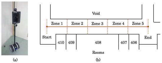
Figure 9.
Human-symbolic autonomous locomotion robot in an actual environment: (a) Mobile robot Double and (b) Experimental environment.
Because the robot had no dedicated camera as the default, we obtained images using a built-in camera in the tablet computer attached to the head part of the robot. The major camera specifications are shown in Table 6. The image resolution and frame rate are, respectively, 472 × 628 pixel and 30 fps. Obtained images are transmitted to a monitoring laptop computer in real time via Wi-Fi. During the experiment, dropped image frames occurred depending on radio wave conditions. We removed these images from the benchmark datasets.
Table 6.
Major camera specifications of the Double mobile robot.
Figure 9b depicts the route for the robot locomotion for capturing time-series images. As an experimental site, we used a corridor in our university building. The left side of the forward direction contains a void area with a part of an atrium from the ground floor to the ceiling with lighting windows. The right side contains laboratories for students and personal office rooms for professors with a different room size.
The length and wide of the corridor, respectively, 38.4 m and 2.1 m, which was sufficient for straight locomotion of the robot. For position recognition, we divided the corridor into five zones of equal length: Zones 1–5. We manually operated the robot using a keyboard on a laptop computer after training in advance. The operational repetition made it possible to move the robot with a constant speed without extreme meandering during image acquisition.
6.2. Dataset Details
Regarding the memory resource capacity and a computational processing cost, we converted captured video images in 30 fps to static images in 10 frame intervals. Figure 10 depicts sample images in respective zones. The images from the left to the right correspond to Zones 1–5. The upper and lower images respectively correspond to those with and without humans. The right-side images contain several objects, such as posters and doors, as VL candidates. The left side contains few objects: merely fire hydrants in the colonnade.
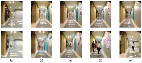
Figure 10.
Sample images in each zone. Images from (a) to (e) correspond to Zones 1–5. Upper and lower images respectively correspond to those with and without humans.
We divided datasets into two types: with humans and without humans in the images. The robot moved in respective zones with constant speed. Regarding robustness for environmental changes related to illumination patterns, we obtained datasets on different dates. Although the periodic variation is included, the mean dataset length is approximately 90 s. We deleted images that contain wireless communication errors from the datasets. The benchmark comprises 12 datasets named Datasets A–K with humans used for evaluation and two datasets without humans used for parameter optimization for our method.
6.3. Feature Extraction
Figure 11 depicts feature extraction results for the respective mask images. For our method, AKAZE features are extracted from with high saliency and without human regions excluded using HOG. We described VL features with no human effect. Figure 11e depicts extracted AKAZE features that are distributed densely on humans and posters installed on the left side of the wall.
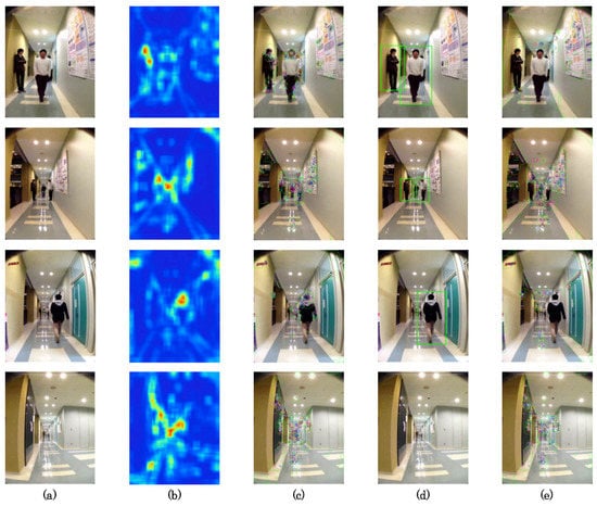
Figure 11.
Feature extraction results in Zone 4: (a) , (b) , (c) AKAZE on , (d) , (e) AKAZE on .
Figure 12 depicts feature extraction result images in Zones 1–3 and 5. The results of Zone 1 are similar among images because of the lack of humans. Although AKAZE feature points were extracted on a human in Zone 2, they were disappeared in our method. Alternative feature points were extracted in the upper and vertical frames of the door. In Zones 3 and 4, feature points were dense for the posters compared with the humans. Using , no feature points were extracted on the humans. Alternative feature points were extracted from the posters. Although HOG windows were falsely detected for the fluorescent lights on the ceiling in Zone 5, the influence was slight because the bench was recognized as a high-saliency region.
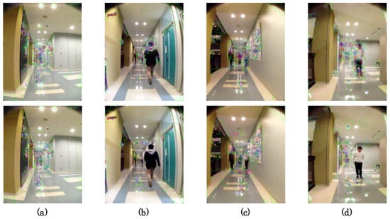
Figure 12.
Feature extraction results: (a) Zones 1, (b) Zone 2, (c) Zone 3, and (d) Zone 5. Colored circles represent AKAZE feature points with scale and orientation.
6.4. Parameter Optimization
Our proposed method based on machine learning algorithms is sensitive for some major parameters that affect recognition accuracies directly. As a preliminary experiment before the evaluation experiment, we optimized three major parameters: the number of SOM mapping units as codebook dimensions, the number of CPN mapping units as the resolution of CMs, and the number of CPN learning iterations for the measure of learning convergence. Regarding appeared frequencies and patterns of humans for this optimization, we used two datasets without humans in all images. As the evaluation criteria, we used LOOCV same at the former experiment. For this validation pattern, one dataset was used for learning and other datasets for testing, in five zones.
Figure 13 depicts the optimization result of codebook dimensions. The codebook size was changed from 16 units to 512 units steps by square numbers. Although recognition accuracies were improved according the increased number of codebooks, the highest recognition accuracy reached to 75.3% in 64 units. From this codebook size, the accuracies were reduced slightly. Although the accuracy reached 1.1% lower than the highest accuracy in 512 units, the accuracy dropped 21.5% lower in 1024 units.
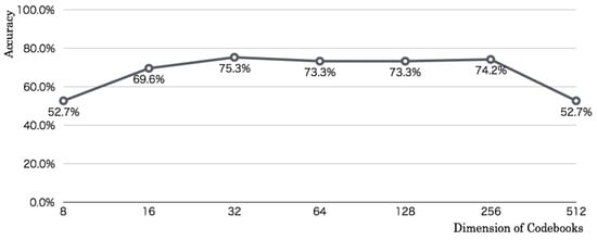
Figure 13.
Relation between codebook dimensions and accuracies.
Figure 14 depicts the optimization results of mapping units on CMs. The unit size was changed from 10 × 10 units to 50 × 50 units, with steps by 10 × 10 units. The respective maximum and minimum recognition accuracies were 69.6% and 65.3%, which was merely a 4.3 percentage point difference. The recognition accuracy on 30 × 30 units was 69.6% which was the same as that on 100 × 100 units. For reference, the accuracy of 100 × 100 units was unsuitable for robot vision applications because real-time processing must be done in combination with memory capacity and in consideration of computational processing time. Therefore, we selected the smaller size for calculation load and a memory size.
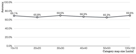
Figure 14.
Relation between CM sizes and accuracies.
Figure 15 presents the optimization results of CPN learning iterations. We evaluated recognition accuracies in six patterns: ( 2, 3, 4, and 5) and ( 3 and 4) iterations. According to increased iterations, the accuracies increased to iterations and reached maximum accuracy of 69.6%. The accuracies decreased according to increased iterations more than iterations. We considered excessive over-fitting for the extended locomotion distance. We assumed that the optimum value of learning iterations changed according to increased images and applied their contents for learning and testing.
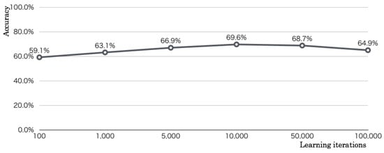
Figure 15.
Relation between learning iterations and accuracies.
6.5. Experimental Results
Figure 16 depicts CMs generated as learning results for each dataset combination. The thermographic color bars on the right side of the maps correspond to Zones 1–5. Category colors are assigned according to thermographic color patterns defined by color temperature. Herein, the low color temperature in blue and high color temperature in red respectively correspond to Zones 1 and 5. CMs created clusters according to similarity of respective categories based on neighborhood and WTA learning. For complex features, similar categories were distributed as partial clusters separated in several regions. The distribution characteristics in each CM addressed that the complexity of VLs corresponded to position recognition.
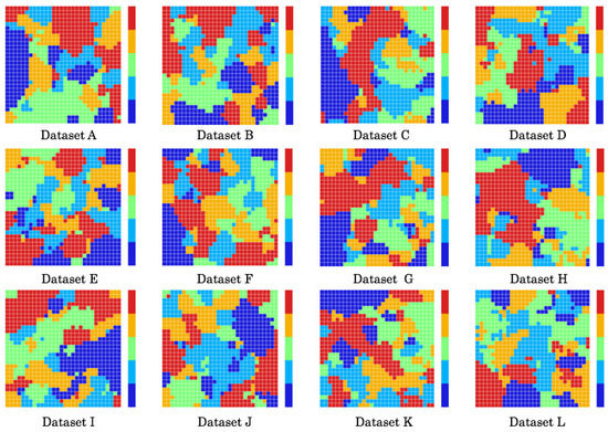
Figure 16.
CMs for each dataset combination.
Figure 17 depicts test results for all datasets. Color patterns correspond to color temperatures of respective scenes on the CMs, as shown in Figure 16. Correct recognition is defined as sequential changes from low color temperature through high color temperature according to robot locomotion. The experimentally obtained results included false recognition partially that were depicted as mixed color patterns.
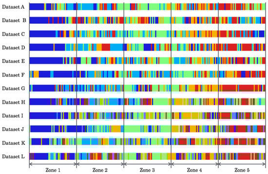
Figure 17.
Test results for all datasets. Color patterns correspond to the CMs.
Table 7 presents recognition accuracies in each test dataset as evaluated using LOOCV. The second and third rows respectively present recognition accuracies of our method and the comparison method without that is defined using the mask image as
Table 7.
Recognition accuracies of our method and comparison method without .
The comparison method extracted AKAZE feature points from .
The mean recognition accuracy of our method was 49.9%. The highest and lowest recognition accuracies were, respectively, 60.9% for Dataset G and 38.2% for Dataset B. The 22.7% difference of the accuracies includes scene complexity and environmental diversity of human movements on each image capturing date.
The mean recognition accuracy of the comparison method was 46.7%. Although the method used the same dataset, the accuracy was 3.2 percentage points lower than that using our method. The highest and lowest recognition accuracies were, respectively, 54.2% for Dataset A and 35.1% for Dataset F. The difference of the accuracies was 19.1% that corresponded to 3.6 percentage points lower accuracy than that of our method.
6.6. Confusion Matrix Analysis
We analyzed false recognition details of our method and the comparison method using a confusion matrix measure. Table 8 denotes confusion matrixes in each recognition result. The confusion matrix of our method, as shown in the left table, is the sum of all LOOCV results for 12 datasets. For the 540 images in Zone 1, which is the highest recognition accuracy, false recognition occurred for 173 images: 61 images for Zone 2, 42 images for Zone 3, 39 images for Zone 4, and 31 images for Zone 5. For this experiment, false recognition occurred in neighbor zones because we restricted the robot mobility to have constant and linear velocity.
Table 8.
Confusion matrixes.
6.7. Discussion
The camera mounted on this robot was set to the forward direction. For this restriction, Zone 1 contains all features of other four zones. In contrast, those zones contain no feature of Zone 1. According to robot locomotion, overlapped features among zones are decreased. In Zone 5, no features of other zones exist because of this restriction. Recognition of Zone 1 was the most difficult of the five zones. However, as a characteristic of the datasets, people in each scene are not increased. The number of persons captured within the visible range is greater in Zones 3 and 4 in front of the laboratory. The recognition accuracy in Zone 1, which has small human influence, was found to be higher than those of other zones because of the overlapping VL proportion and reduced number of people.
Among the five zones, Zone 4 was found to have the lowest recognition accuracy. For the total 540 images, 216 images were recognized correctly for Zone 4. The false recognition to Zone 3, which is the previous zone of Zone 4, is the maximum: the 103 images are nearly half of the correct images. As shown in Figure 9b, monotonous scenes were continued in the corridor, especially in Zones 2–4, as shown sample images in Figure 10. For these zones, VLs are extracted from posters that consist of various contents, and doors, and which are used for the same structure and patterns in each room. We consider that it is a challenging task to recognize these zones compared with Zones 1 and 5. As shown in Figure 10, visual features in these zones include chairs, vending machines, a rest space on the right side with a corner, and a walkway along with a void area.
The comparison result depicted in the right table demonstrates similar tendencies to those found for the result of our method. Recognition images were decreased, especially in Zones 2–5, which have a larger human influence. In Zone 1, falsely recognized images were fewer than those obtained using our method. As the preliminary experiment showed, this result is related to the HOG accuracy. The FPR occurred more frequently in Zone 1 than in other zones. The lighting on the ceiling, which is inappropriate as a VL candidate, was falsely recognized as people in Zone 1. The FPs were few because people clearly were present in the environment. We consider that the uniformity of human appearance frequency of humans in the datasets is undesirable for a benchmark. Actually, places for which human influence is changed to large or small are actual environments. For this evaluation experiment, robot locomotion was limited to five zones with total length of 38.4 m. To expand applicable environments with obtaining benchmark datasets, we expect to develop a method that learns comprehensively including the appearance frequency of people and recognition of positions. Regarding false recognition for each zone, we infer that further study is necessary for boundaries and zones recognized as a category.
Although our evaluation target was all images of the datasets while the robot was moving, VL features have no sudden change in the boundaries of switched zones. For the continuous variation of image features, learning slight differences with teaching signals in supervised learning is not only a challenging task for semantic scene recognition. It is also difficult because of a lack of practical use. For our experiment, we divided the route into five zones of fixed length. We will examine a method that divides boundaries with semantic categories as zones using unsupervised and incremental learning algorithms. According to expanding applicable environments for position estimation at any zone including boundaries, we will reuse our existing method [40] for acquisition of world images by a mobile robot. For this method, the robot recognized a position using time-series image sequences obtained using a monocular camera with a pan function.
Finally, we have no comparison results with other state-of-the-art methods. Our proposed method uses CPNs for recognition. We consider that it is possible to replace state-of-the-art methods including deep learning according to the progress of machine learning algorithms.
7. Conclusions
This paper presented a VL-based scene recognition method for the robustness of human influence. The proposed method described VL features using AKAZE on SMs after excepting human regions using HOG. We used SOMs to create codebooks as visual words and CPNs for mapping features into a low dimension space as a CM based on neighborhood and WTA learning. As a preliminary experiment, we conducted evaluation experiments using KTH-IDOL2 benchmark datasets with three illumination conditions. The experimentally obtained results using leave-one-out cross validation (LOOCV) revealed that recognition accuracy of high-saliency feature points was higher than that of low-saliency feature points. Moreover, we conducted evaluation experiments using EPFL benchmark datasets for detecting pedestrians as the basic performance evaluation of HOG detectors. Furthermore, we created our original benchmark datasets including humans in time-series images obtained using a mobile robot. As evaluated using LOOCV, the recognition accuracies of our method and the comparison method were, respectively, 49.9% and 46.7%, which represented a 3.2 percentage point superiority of our method. The analysis using a confusion matrix revealed that false recognition occurred in neighboring zones. This trend was reduced according to the zone separations according to the robot locomotion.
Future work should include expanding benchmark dataset acquisition, application to large-scale environments including various appearance patterns and frequencies of people, incorporation of incremental learning approaches, attending deep learning mechanisms with low computational burden, invariant of VL feature changes near zone boundaries, combined with a map created using SLAM as visual SLAM, considering VGI-based landmarks, and position recognition while terminating locomotion as actualizing a human-symbolic robot. Moreover, we would like apply our method to smart homes whose living conditions could be improved by human-centered robot solutions for actualizing smart living and smart cities.
Author Contributions
Conceptualization, H.M. and K.S.; methodology, H.M.; software, H.M.; validation, N.S.; formal analysis, H.M.; investigation, N.S.; resources, H.M.; data curation, K.S.; writing—original draft preparation, H.M.; writing—review and editing, H.M.; visualization, K.S.; supervision, H.M.; project administration, H.M.; funding acquisition, H.M.
Funding
This research was supported by Japan Society for the Promotion of Science (JSPS) KAKENHI Grant Number 17K00384.
Conflicts of Interest
The authors declare no conflict of interest. The funders had no role in the design of the study; in the collection, analyses, or interpretation of data; in the writing of the manuscript, or in the decision to publish the results.
Abbreviations
The following abbreviations are used in this manuscript:
| SLAM | simultaneous localization and mapping |
| LRFs | laser range finders |
| VL | visual landmark |
| SMG | saliency map graph |
| SMs | salience maps |
| SIFT | scale-invariant feature transform |
| SVMs | support vector machines |
| AR | augmented reality |
| GVG | generalized Voronoi graph |
| PIRFs | position invariant robust features |
| AKAZE | accelerated KAZE |
| HOG | histogram of oriented gradients |
| ACMNs | adaptive category mapping networks |
| CM | category map |
| SOMs | self-organizing maps |
| CPNs | counter propagation networks |
| ART | adaptive resonance theory |
| FMs | feature maps |
| WTA | winner-take-all |
| GT | ground truth |
| PA | printer area |
| BO | one-person office |
| EO | two-person office |
| KT | kitchen |
| CR | corridor |
| LOOCV | leave-one-out cross-validation |
| FPGAs | field-programmable gate arrays |
| TPR | true positive rate |
| TP | true positive |
| FP | false positive |
| FNR | false negative rate |
| FN | false negative |
| VGI | volunteered geographic information |
| BGVS | Graph Based Visual Saliency |
| HTM | Hierarchical Temporal Memory |
References
- Dissanayake, G.; Newman, P.; Clark, S.; Durrant-Whyte, H.F.; Csorba, M. An Experimental and Theoretical Investigation into Simultaneous Localisation and Map Building (SLAM). Exp. Robot. 2000, 265–274. [Google Scholar] [CrossRef]
- Ishikoori, Y.; Madokoro, H.; Sato, K. Semantic Position Recognition and Visual Landmark Detection with Invariant for Human Effect. In Proceedings of the 2017 IEEE/SICE International Symposium on System Integration (SII), Taipei, Taiwan, 11–14 December 2017. [Google Scholar]
- Tokuhara, K.; Madokoro, H.; Sato, K. Semantic Indoor Scenes Recognition Based on Visual Saliency and Part-Based Features. In Proceedings of the 2017 IEEE/SICE International Symposium on System Integration (SII), Taipei, Taiwan, 11–14 December 2017. [Google Scholar]
- Desouza, G.N.; Kak, A.C. Vision for mobile robot navigation: A survey. IEEE Trans. Pattern Anal. Mach. Intell. 2002, 24, 237–267. [Google Scholar] [CrossRef]
- Li, F.F.; Perona, P. A Bayesian Hierarchical Model for Learning Natural Scene Categories. Proc. Comput. Vis. Pattern Recognit. 2005, 2, 524–531. [Google Scholar] [CrossRef]
- Shokoufandeha, A.; Marsicb, I.; Dickinsona, S.J. View-Based Object Recognition Using Saliency Maps. Image Vis. Comput. 1999, 17, 445–460. [Google Scholar] [CrossRef]
- Walthera, D.; Koch, C. Modeling Attention to Salient Proto-Objects. Neural Netw. 2006, 19, 1395–1407. [Google Scholar] [CrossRef]
- Itti, L.; Koch, C.; Niebur, E. A Model of Saliency-Based Visual Attention for Rapid Scene Analysis. IEEE Trans. Pattern Anal. Mach. Intell. 1998, 20, 1254–1259. [Google Scholar] [CrossRef]
- Lowe, D.G. Object Recognition from Local Scale-Invariant Features. In Proceedings of the Seventh IEEE International Conference on Computer Vision, Kerkyra, Greece, 20–27 September 1999. [Google Scholar]
- Harel, J.; Koch, C.; Perona, P. Graph-based visual saliency. Adv. Neural Inf. Process. Syst. 2006, 19, 545–552. [Google Scholar] [CrossRef]
- Kostavelis, I.; Nalpantidis, L.; Gasteratos, A. Object Recognition Using Saliency Maps and HTM Learning. In Proceedings of the 2012 IEEE International Conference on Imaging Systems and Techniques, Manchester, UK, 16–17 July 2012. [Google Scholar]
- Kostavelis, I.; Gasteratos, A. Learning spatially semantic representations for cognitive robot navigation. Robot. Autom. Syst. 2013, 61, 1460–1475. [Google Scholar] [CrossRef]
- Kostavelis, I.; Gasteratos, A. Semantic mapping for mobile robotics tasks: A survey. Robot. Autom. Syst. 2015, 66, 86–103. [Google Scholar] [CrossRef]
- Fernandes, C.S.; Campos, M.F.M.; Chaimowicz, L. A Low-Cost Localization System Based on Artificial Landmarks. In Proceedings of the 2012 Brazilian Robotics Symposium and Latin American Robotics Symposium, Fortaleza, Brazil, 16–19 Octorber 2012. [Google Scholar]
- Chang, C.K.; Siagian, C.; Itti, L. Mobile Robot Vision Navigation and Localization Using Gist and Saliency. In Proceedings of the 2010 IEEE/RSJ International Conference on Intelligent Robots and Systems, Taipei, Taiwan, 18–22 Octorber 2010. [Google Scholar]
- Hayet, J.B.; Lerasle, F.; Devy, M. A Visual Landmark Framework for Mobile Robot Navigation. Image Vis. Comput. 2007, 25, 1341–1351. [Google Scholar] [CrossRef]
- Sala, P.; Sim, R.; Shokoufandeh, A.; Dickinson, S. Landmark Selection for Vision-Based Navigation. IEEE Trans. Robot. 2006, 22, 334–349. [Google Scholar] [CrossRef]
- Hayet, J.B.; Esteves, C.; Devy, M. Qualitative Modeling of Indoor Environments from Visual Landmarks and Range Data. In Proceedings of the IEEE/RSJ International Conference on Intelligent Robots and Systems, Lausanne, Switzerland, 30 September–4 Octorber 2002. [Google Scholar]
- Se, S.; Lowe, D.; Little, J. Mobile Robot Localization and Mapping with Uncertainty Using Scale-Invariant Visual Landmarks. Int. J. Robot. Res. 2002, 21, 735–758. [Google Scholar] [CrossRef]
- Livatino, S.; Madsen, C.B. Automatic Selection of Visual Landmark for Mobile Robot Navigation. In Proceedings of the Seventh Danish Conference on Pattern Recognition and Image Analysis, Copenhagen, Denmark, August 1998. [Google Scholar]
- Bestgen, A.K.; EdlerLars, D.; Kuchinke, L.; Dickmann, F. Analyzing the Effects of VGI-based Landmarks on Spatial Memory and Navigation Performance. Ger. J. Artif. Intell. 2017, 31, 179–183. [Google Scholar] [CrossRef]
- Kawewong, A.; Tangruamsub, S.; Hasegawa, O. Position-invariant Robust Features for Long-term Recognition of Dynamic Outdoor Scenes. IEICE Trans. Inf. Syst. 2010, 93, 2587–2601. [Google Scholar] [CrossRef]
- Noguchi, H.; Yamada, T.; Mori, T.; Sato, T. Human Avoidance Path Planning based on Massive People Trajectories. J. Robot. Soc. J. 2012, 30, 684–694. [Google Scholar] [CrossRef]
- Alcantarilla, P.F.; Nuevo, J.; Batoli, A. Fast Explicit Diffusion for Accelerated Features in Nonlinear Scale Spaces. IEEE Trans. Pattern Anal. Mach. Intell. 2011, 34, 1281–1298. [Google Scholar]
- Dalal, N.; Triggs, B. Histograms of oriented gradients for human detection. In Proceedings of the 2005 IEEE Computer Society Conference on Computer Vision and Pattern Recognition, San Diego, CA, USA, 20–25 June 2005. [Google Scholar]
- Madokoro, H.; Shimoi, N.; Sato, K. Adaptive Category Mapping Networks for All-Mode Topological Feature Learning Used for Mobile Robot Vision. In Proceedings of the 23rd IEEE International Symposium on Robot and Human Interactive Communication, Edinburgh, UK, 25–29 August 2014. [Google Scholar]
- Kohonen, T. Self-Organizing Maps; Springer: Berlin/Heidelberg, Germany, 1995. [Google Scholar]
- Hetch-Nielsen, R. Counterpropagation networks. Appl. Opt. 1987, 26, 4979–4983. [Google Scholar] [CrossRef]
- Carpenter, G.A.; Grossberg, S. ART 2: Stable Self-Organization of Pattern Recognition Codes for Analog Input Patterns. Appl. Opt. 1987, 26, 4919–4930. [Google Scholar] [CrossRef]
- Oliva, A.; Torralba, A. Modeling the Shape of the Scene: A Holistic Representation of the Spatial Envelope. Int. J. Comput. Vis. 2001, 42, 145–175. [Google Scholar] [CrossRef]
- Alcantarilla, P.F.; Bartoli, A.; Davison, A.J. KAZE Features. In Proceedings of the ECCV 2012—12th European Conference on Computer Vision, Florence, Italy, 7–13 October 2012. [Google Scholar]
- Koch, C.; Ullman, S. Shifts in Selective Visual Attention: Towards the Underlying Neural Circuitry. Matters Intell. 1987, 188, 115–141. [Google Scholar] [CrossRef]
- Luo, J.; Pronobis, A.; Caputo, B.; Jensfelt, P. Incremental learning for place recognition in dynamic environments. In Proceedings of the 2007 IEEE/RSJ International Conference on Intelligent Robots and Systems, San Diego, CA, USA, 29 October–2 November 2007. [Google Scholar]
- Zhou, B.; Lapedriza, A.; Khosla, A.; Oliva, A.; Torralba, A. Places: A 10 million Image Database for Scene Recognition. IEEE Trans. Pattern Anal. Mach. Intell. 2018, 40, 1452–1464. [Google Scholar] [CrossRef] [PubMed]
- Kohavi, R. A Study of Cross-Validation and Bootstrap for Accuracy Estimation and Model Selection. Proc. Int. J. Conf. Artif. Intell. 1995, 2, 1137–1143. [Google Scholar]
- Madokoro, H.; Sato, K.; Ishii, M. FPGA Implementation of Back-Propagation Neural Networks for Real-Time Image Processing. J. Comput. 2013, 8, 559–566. [Google Scholar] [CrossRef]
- Kalms, L.; Elhossini, A.; Juurlink, B. FPGA based hardware accelerator for KAZE feature extraction algorithm. In Proceedings of the 2016 International Conference on Field-Programmable Technology (FPT), Xi’an, China, 7–9 December 2016. [Google Scholar]
- Fleuret, F.; Berclaz, J.; Lengagne, R.; Fua, P. Multi-Camera People Tracking with a Probabilistic Occupancy Map. IEEE Trans. Pattern Anal. Mach. Intell. 2008, 30, 267–282. [Google Scholar] [CrossRef] [PubMed]
- Powers, D. Evaluation: From Precision, Recall and F-Factor to ROC, Informedness, Markedness & Correlation. J. Mach. Learn. Tech. 2011, 2, 37–63. [Google Scholar] [CrossRef]
- Madokoro, H.; Sato, K.; Ishii, M. Acquisition of World Image and Self-Localization Using Sequential View Images. Syst. Comput. Jpn. 2003, 34, 68–78. [Google Scholar] [CrossRef]


© 2019 by the authors. Licensee MDPI, Basel, Switzerland. This article is an open access article distributed under the terms and conditions of the Creative Commons Attribution (CC BY) license (http://creativecommons.org/licenses/by/4.0/).