
Investigating the Impact of Triangle and Quadrangle Mesh Representations on AGV Path Planning for Various Indoor Environments: With or Without Inflation


Abstract
:1. Introduction
- Showing that the type of environment representation has a direct impact on path planning, and quantifying this by a metric.
- Presenting the results showing the pros and cons of each representation when considering the inflation layer
2. Problem Formulation and Assumption
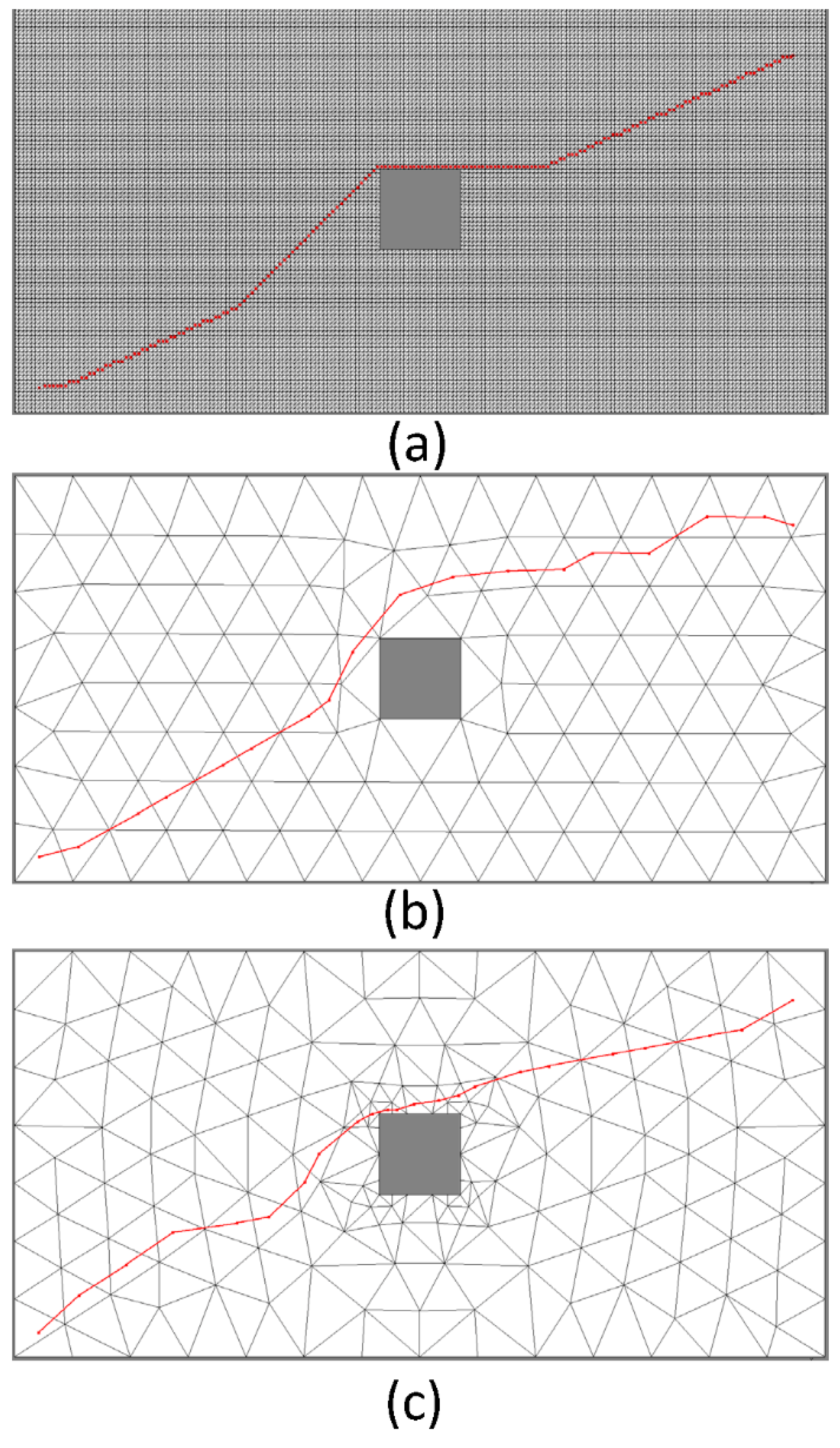
3. Environment Modelling for Navigation
4. Methodology
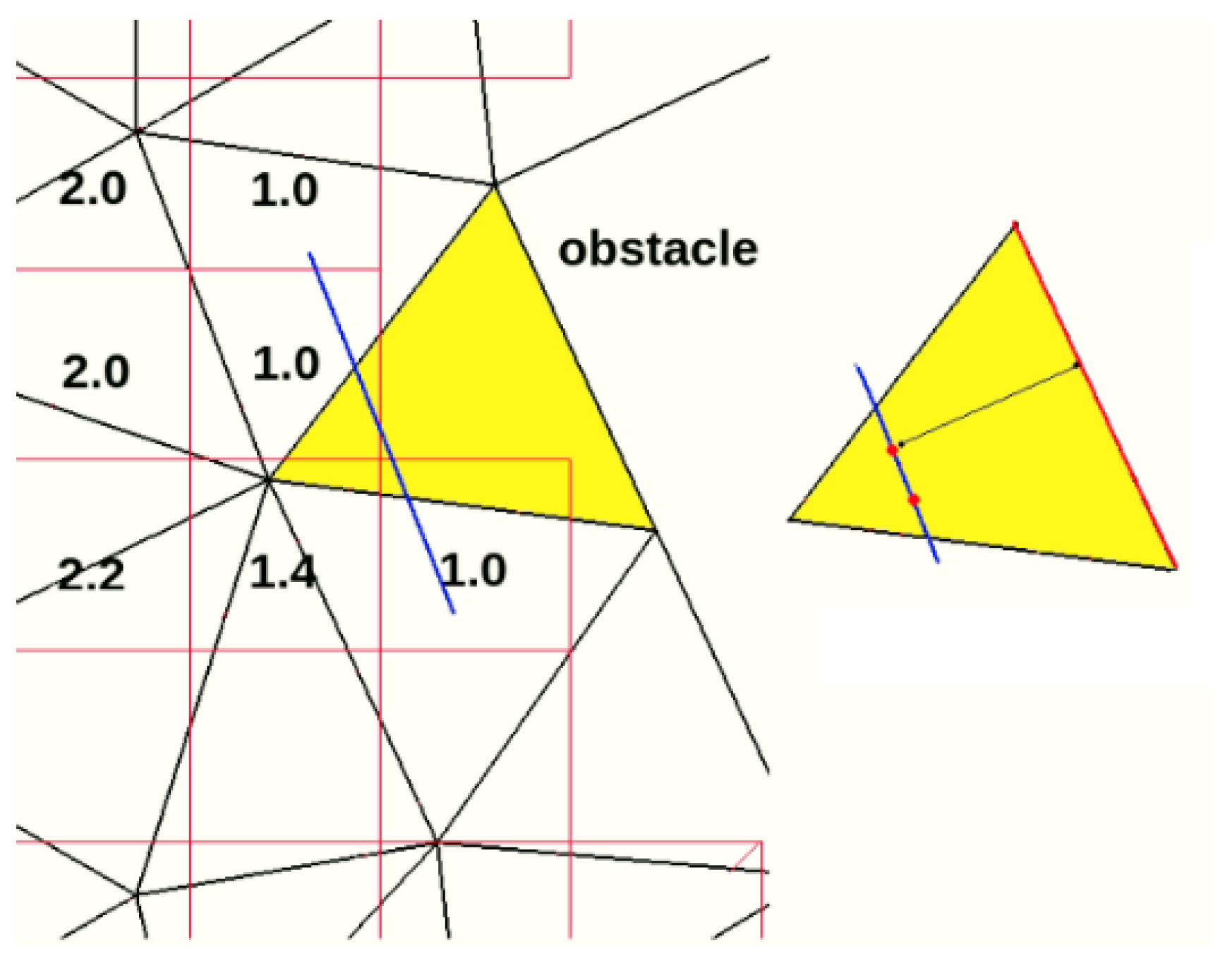
4.1. Pure Decomposition
4.2. Decomposition of Inflation Layer
5. Results and Discussion
5.1. Platform for Experiment
- QUAD mesh (GRID Nx × Ny): four cell sizes (GRID 100 × 50, GRID 120 × 60, GRID 160 × 80, and GRID 200 × 100) are considered for this mesh where Nx and Ny are the number of cells in horizontal and vertical directions.
- ITM: four cell sizes (ITM-700, ITM-500, ITM-300, ITM-100) are also considered for this mesh. ITM-100 refers to a triangle with an average of 100 mm edges. For some environments where this was not applicable, larger triangles and smaller ones were used.
- Varying-size ITM (VITM): Concerning this mesh, ITM-100-700 is utilized. This size refers to a triangular mesh with an average edge size of 700 mm, which has been refined to size 100 mm in some places. When confronting narrow passages, VITM-50-700 or VITM-30-700 have also been utilized.
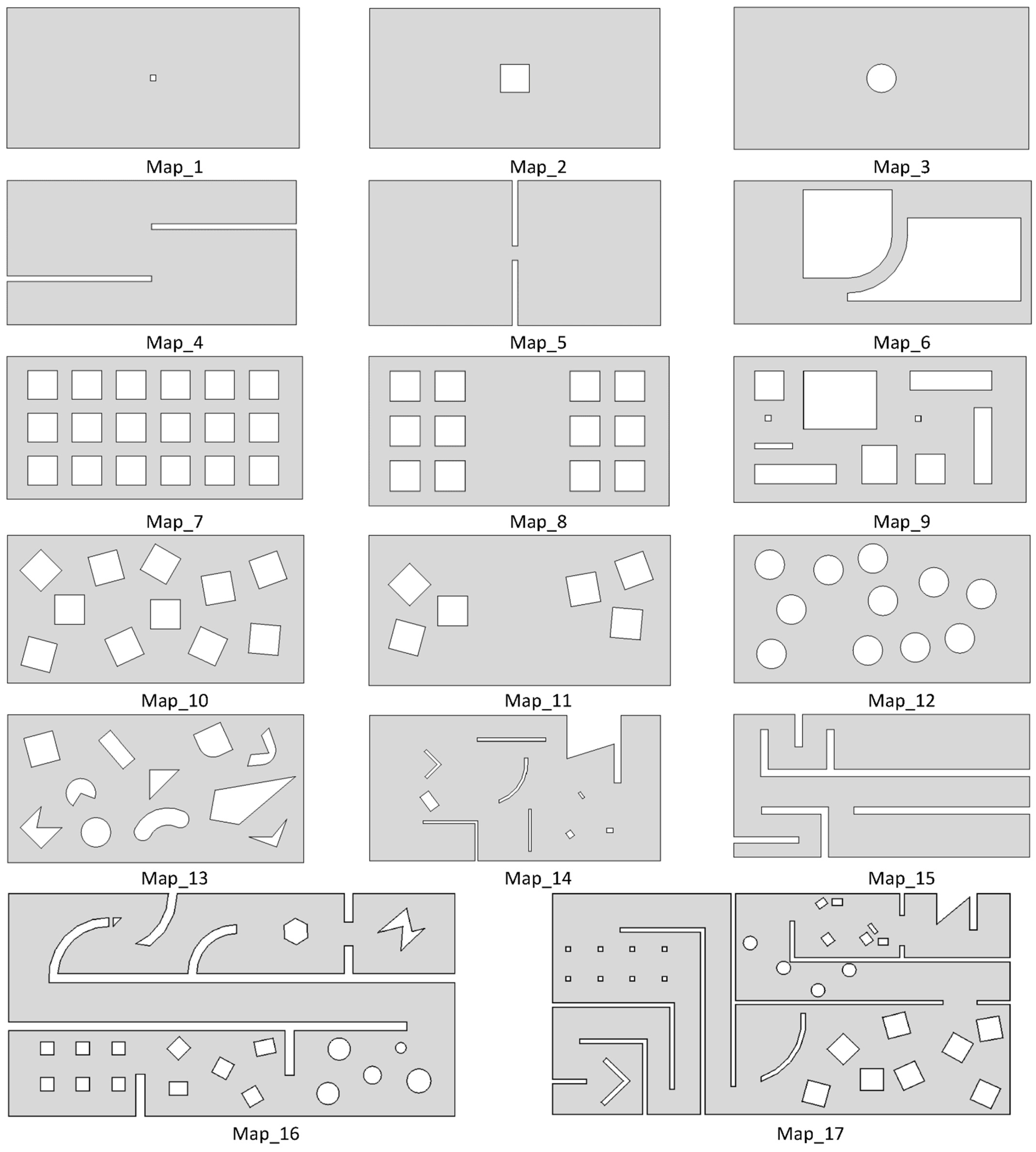
- Area with single obstacle: Map_1 (small-size obstacle), Map_2 (medium-size polygonal obstacle), Map_3 (medium-size circular obstacle)
- Space with dividers (Map_4)
- Narrow passage (Map_5)
- Curvilinear passage: Map6
- Area with regular multi-obstacles: Map_7, Map_8 (two groups), Map_9 (different size)
- Area with irregular multi-obstacles: Map_10, Map_11 (two groups), Map_12 (circular), Map_13 (different shapes)
- Hybrid with wide space: Map_14
- Corridor and dividers: Map_15
- Hybrid narrow space environments: Map_16, Map_17 (including all the previous environments)
5.2. Result—Environment and Representations
5.3. Result—Inflation Effect on the Representations
5.4. Results—Discussion
- In multi-robot sizes conditions, when is not possible to apply the offsetting method.
- Some changes in the environment make it necessary to apply online inflation to the map, and not by offsetting the obstacles in the primary map.
- There are narrow passages for a robot which makes ITM representation useless.
6. Conclusions and Future Work
Author Contributions
Funding
Institutional Review Board Statement
Informed Consent Statement
Data Availability Statement
Acknowledgments
Conflicts of Interest
Appendix A
- ₋ Figure A1: All defined environments
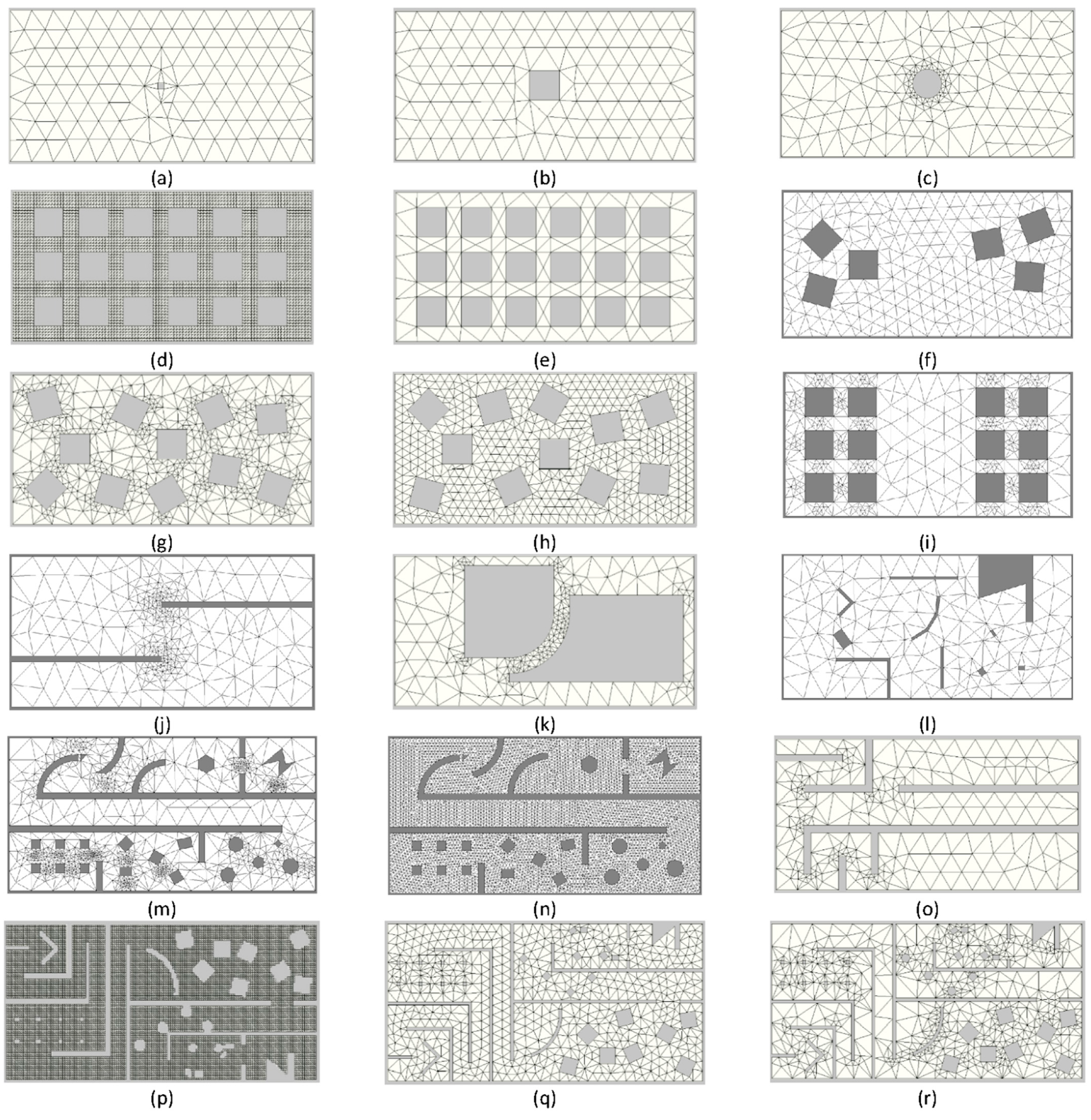
- ₋ Figure A2: Sample of various representation types and sizes
- ₋ Table A1: Result without consideration of inflation for all environments and representations
- ₋ Table A2: Result with consideration of inflation for all environments and representations


| Map Name | Representations | S (300, 300) G (9600, 4400) | Parameters | Single Criteria | |||
|---|---|---|---|---|---|---|---|
| Type | Size | Inflation | Length mm | Min Distance mm | Complexity | f Cost Function | |
| Map_1 | QUAD | GRID 100 × 50 | 0 | 10,986 | 75 | 2269 | 0.042 |
| QUAD | GRID 120 × 60 | 0 | 11,022 | 125 | 3160 | 0.056 | |
| QUAD | GRID 160 × 80 | 0 | 11,007 | 75 | 5463 | 0.095 | |
| QUAD | GRID 200 × 100 | 0 | 10,992 | 25 | 8359 | 0.143 | |
| ITM | 700 | 0 | 10,451 | 133 | 114 | 0.005 | |
| ITM | 500 | 0 | 10,433 | 275 | 168 | 0.006 | |
| ITM | 300 | 0 | 10,381 | 46 | 358 | 0.010 | |
| ITM | 100 | 0 | 10,329 | 275 | 1644 | 0.031 | |
| VITM | 100_700 | 0 | 10,292 | 1 | 118 | 0.008 | |
| Map_2 | QUAD | GRID 100 × 50 | 0 | 10,986 | 25 | 2251 | 0.042 |
| QUAD | GRID 120 × 60 | 0 | 11,022 | 25 | 3206 | 0.058 | |
| QUAD | GRID 160 × 80 | 0 | 11,007 | 25 | 5452 | 0.097 | |
| QUAD | GRID 200 × 100 | 0 | 10,992 | 25 | 8323 | 0.145 | |
| ITM | 700 | 0 | 10,749 | 155 | 134 | 0.006 | |
| ITM | 500 | 0 | 10,375 | 25 | 153 | 0.006 | |
| ITM | 300 | 0 | 10,484 | 46 | 369 | 0.010 | |
| ITM | 100 | 0 | 10,570 | 125 | 3030 | 0.055 | |
| VITM | 100_700 | 0 | 10,521 | 19 | 177 | 0.007 | |
| Map_3 | QUAD | GRID 100 × 50 | 0 | 10,986 | 25 | 2255 | 0.042 |
| QUAD | GRID 120 × 60 | 0 | 11,022 | 25 | 3049 | 0.056 | |
| QUAD | GRID 160 × 80 | 0 | 11,007 | 25 | 5269 | 0.093 | |
| QUAD | GRID 200 × 100 | 0 | 10,992 | 25 | 8117 | 0.141 | |
| ITM | 700 | 0 | 10,521 | 17 | 106 | 0.006 | |
| ITM | 500 | 0 | 10,559 | 75 | 190 | 0.007 | |
| ITM | 300 | 0 | 10,456 | 3 | 444 | 0.012 | |
| ITM | 100 | 0 | 10,399 | 19 | 2191 | 0.041 | |
| VITM | 100_700 | 0 | 10,394 | 40 | 173 | 0.007 | |
| Map_4 | QUAD | GRID 100 × 50 | 0 | 12,416 | 25 | 2695 | 0.051 |
| QUAD | GRID 120 × 60 | 0 | 12,409 | 25 | 3707 | 0.069 | |
| QUAD | GRID 160 × 80 | 0 | 12,340 | 25 | 6468 | 0.117 | |
| QUAD | GRID 200 × 100 | 0 | 12,293 | 25 | 10,078 | 0.179 | |
| ITM | 700 | 0 | 12,565 | 116 | 164 | 0.007 | |
| ITM | 500 | 0 | 12,438 | 75 | 295 | 0.010 | |
| ITM | 300 | 0 | 12,222 | 75 | 747 | 0.017 | |
| ITM | 100 | 0 | 12,031 | 13 | 5613 | 0.102 | |
| VITM | 100_700 | 0 | 11,953 | 15 | 412 | 0.012 | |
| Map_5 | QUAD | GRID 100 × 50 | 0 | 10,986 | 75 | 2102 | 0.039 |
| QUAD | GRID 120 × 60 | 0 | 11,022 | 25 | 2917 | 0.053 | |
| QUAD | GRID 160 × 80 | 0 | 11,007 | 25 | 5064 | 0.090 | |
| QUAD | GRID 200 × 100 | 0 | 10,992 | 25 | 7812 | 0.136 | |
| ITM | 700 | 0 | 10,294 | 87 | 92 | 0.005 | |
| ITM | 500 | 0 | 10,285 | 125 | 153 | 0.006 | |
| ITM | 300 | 0 | 10,339 | 133 | 308 | 0.009 | |
| ITM | 100 | 0 | 10,379 | 116 | 2316 | 0.043 | |
| VITM | 100_700 | 0 | 10,404 | 125 | 220 | 0.007 | |
| Map_6 | QUAD | GRID 100 × 50 | 0 | 11,630 | 25 | 1579 | 0.053 |
| QUAD | GRID 120 × 60 | 0 | 11,657 | 25 | 2134 | 0.070 | |
| QUAD | GRID 160 × 80 | 0 | 11,592 | 25 | 3726 | 0.116 | |
| QUAD | GRID 200 × 100 | 0 | 11,519 | 25 | 5740 | 0.175 | |
| ITM | 700 | 0 | 11,109 | 46 | 94 | 0.009 | |
| ITM | 500 | 0 | 11,403 | 75 | 188 | 0.012 | |
| ITM | 300 | 0 | 11,048 | 46 | 360 | 0.017 | |
| ITM | 100 | 0 | 11,065 | 14 | 2859 | 0.091 | |
| VITM | 100_700 | 0 | 11,052 | 25 | 275 | 0.015 | |
| Map_7 | QUAD | GRID 100 × 50 | 0 | 12,386 | 25 | 2289 | 0.066 |
| QUAD | GRID 120 × 60 | 0 | 12,380 | 25 | 2995 | 0.085 | |
| QUAD | GRID 160 × 80 | 0 | 12,327 | 25 | 5502 | 0.150 | |
| QUAD | GRID 200 × 100 | 0 | 12,173 | 25 | 8388 | 0.225 | |
| ITM | 700 | 0 | 12,760 | 46 | 190 | 0.012 | |
| ITM | 500 | 0 | 12,357 | 20 | 226 | 0.013 | |
| ITM | 300 | 0 | 12,233 | 11 | 552 | 0.021 | |
| ITM | 100 | 0 | 11,798 | 0.4 | 4428 | 0.130 | |
| VITM | 100_700 | 0 | 12,031 | 45 | 513 | 0.020 | |
| Map_8 | QUAD | GRID 100 × 50 | 0 | 11,566 | 25 | 2224 | 0.054 |
| QUAD | GRID 120 × 60 | 0 | 11,640 | 25 | 3418 | 0.080 | |
| QUAD | GRID 160 × 80 | 0 | 11,521 | 25 | 5532 | 0.126 | |
| QUAD | GRID 200 × 100 | 0 | 11,511 | 25 | 8836 | 0.199 | |
| ITM | 700 | 0 | 11,938 | 20 | 167 | 0.009 | |
| ITM | 500 | 0 | 11,465 | 27 | 242 | 0.011 | |
| ITM | 300 | 0 | 11,444 | 39 | 611 | 0.019 | |
| ITM | 100 | 0 | 11,181 | 0 | 4737 | 0.117 | |
| VITM | 100_700 | 0 | 11,584 | 5 | 435 | 0.015 | |
| Map_9 | QUAD | GRID 100 × 50 | 0 | 11,408 | 25 | 1705 | 0.046 |
| QUAD | GRID 120 × 60 | 0 | 11,461 | 25 | 2483 | 0.064 | |
| QUAD | GRID 160 × 80 | 0 | 11,373 | 25 | 4069 | 0.102 | |
| QUAD | GRID 200 × 100 | 0 | 11,343 | 25 | 6520 | 0.160 | |
| ITM | 700 | 0 | 11,207 | 31 | 120 | 0.008 | |
| ITM | 500 | 0 | 11,108 | 2 | 190 | 0.011 | |
| ITM | 300 | 0 | 10,921 | 13 | 379 | 0.015 | |
| ITM | 100 | 0 | 10,878 | 10 | 2793 | 0.072 | |
| VITM | 100_700 | 0 | 10,925 | 17 | 315 | 0.013 | |
| Map_10 | QUAD | GRID 100 × 50 | 0 | 11,239 | 25 | 1458 | 0.037 |
| QUAD | GRID 120 × 60 | 0 | 11,189 | 25 | 2252 | 0.055 | |
| QUAD | GRID 160 × 80 | 0 | 11,222 | 25 | 3771 | 0.089 | |
| QUAD | GRID 200 × 100 | 0 | 11,201 | 25 | 5759 | 0.132 | |
| ITM | 700 | 0 | 11,105 | 14 | 119 | 0.008 | |
| ITM | 500 | 0 | 11,149 | 45 | 209 | 0.010 | |
| ITM | 300 | 0 | 11,292 | 2 | 583 | 0.020 | |
| ITM | 100 | 0 | 10,814 | 3 | 2507 | 0.061 | |
| VITM | 100_700 | 0 | 10,854 | 32 | 440 | 0.015 | |
| Map_11 | QUAD | GRID 100 × 50 | 0 | 11,156 | 25 | 1650 | 0.036 |
| QUAD | GRID 120 × 60 | 0 | 11,120 | 25 | 2498 | 0.053 | |
| QUAD | GRID 160 × 80 | 0 | 11,119 | 25 | 4214 | 0.086 | |
| QUAD | GRID 200 × 100 | 0 | 11,119 | 25 | 6395 | 0.128 | |
| ITM | 700 | 0 | 10,500 | 13 | 95 | 0.006 | |
| ITM | 500 | 0 | 10,615 | 45 | 140 | 0.007 | |
| ITM | 300 | 0 | 10,519 | 32 | 356 | 0.011 | |
| ITM | 100 | 0 | 10,550 | 18 | 2998 | 0.062 | |
| VITM | 100_700 | 0 | 10,596 | 21 | 317 | 0.010 | |
| Map_12 | QUAD | GRID 100 × 50 | 0 | 11,069 | 25 | 1651 | 0.039 |
| QUAD | GRID 120 × 60 | 0 | 11,091 | 25 | 2321 | 0.053 | |
| QUAD | GRID 160 × 80 | 0 | 11,058 | 25 | 4066 | 0.089 | |
| QUAD | GRID 200 × 100 | 0 | 11,033 | 25 | 6316 | 0.135 | |
| ITM | 700 | 0 | 10,531 | 4 | 94 | 0.007 | |
| ITM | 500 | 0 | 10,454 | 24 | 153 | 0.008 | |
| ITM | 300 | 0 | 10,369 | 29 | 230 | 0.009 | |
| ITM | 100 | 0 | 10,522 | 24 | 2026 | 0.046 | |
| VITM | 100_700 | 0 | 10,398 | 42 | 299 | 0.011 | |
| Map_13 | QUAD | GRID 100 × 50 | 0 | 11,239 | 25 | 1479 | 0.036 |
| QUAD | GRID 120 × 60 | 0 | 11,189 | 25 | 2366 | 0.055 | |
| QUAD | GRID 160 × 80 | 0 | - | - | - | - | |
| QUAD | GRID 200 × 100 | 0 | 11,201 | 25 | 5999 | 0.132 | |
| ITM | 700 | 0 | 11,048 | 12 | 126 | 0.008 | |
| ITM | 500 | 0 | 11,026 | 44 | 160 | 0.008 | |
| ITM | 300 | 0 | 11,011 | 23 | 494 | 0.015 | |
| ITM | 100 | 0 | 10,891 | 14 | 3802 | 0.086 | |
| VITM | 100_700 | 0 | 11,063 | 21 | 254 | 0.010 | |
| Map_14 | QUAD | GRID 100 × 50 | 0 | 11,903 | 25 | 3025 | 0.060 |
| QUAD | GRID 120 × 60 | 0 | 11,855 | 25 | 4270 | 0.083 | |
| QUAD | GRID 160 × 80 | 0 | 11,918 | 25 | 7623 | 0.145 | |
| QUAD | GRID 200 × 100 | 0 | 11,892 | 25 | 11,932 | 0.225 | |
| ITM | 700 | 0 | 11,568 | 42 | 214 | 0.008 | |
| ITM | 500 | 0 | 11,469 | 46 | 327 | 0.010 | |
| ITM | 300 | 0 | 11,573 | 46 | 771 | 0.019 | |
| ITM | 100 | 0 | 11,346 | 9 | 5936 | 0.114 | |
| VITM | 100_700 | 0 | 11,590 | 5 | 298 | 0.010 | |
| Map_15 | QUAD | GRID 100 × 50 | 0 | 17,192 | 25 | 3118 | 0.068 |
| QUAD | GRID 120 × 60 | 0 | 17,246 | 25 | 4422 | 0.093 | |
| QUAD | GRID 160 × 80 | 0 | 17,031 | 25 | 7472 | 0.153 | |
| QUAD | GRID 200 × 100 | 0 | 16,769 | 25 | 11,676 | 0.235 | |
| ITM | 700 | 0 | 17,764 | 31 | 209 | 0.011 | |
| ITM | 500 | 0 | 18,192 | 46 | 353 | 0.014 | |
| ITM | 300 | 0 | 17,480 | 29 | 919 | 0.025 | |
| ITM | 100 | 0 | 16,593 | 8 | 7053 | 0.145 | |
| VITM | 100_700 | 0 | 16,786 | 1 | 403 | 0.020 | |
| Map_16 | QUAD | GRID 200 × 100 | 0 | 29,830 | 25 | 13,978 | 0.303 |
| ITM | 100 | 0 | 30,072 | 0 | 8215 | 0.219 | |
| VITM | 28_700 | 0 | 30,183 | 5 | 1538 | 0.045 | |
| Map_17 | QUAD | GRID 120 × 60 | 0 | 32,876 | 25 | 5157 | 0.119 |
| QUAD | GRID 160 × 80 | 0 | 32,308 | 25 | 9484 | 0.206 | |
| QUAD | GRID 200 × 100 | 0 | 32,075 | 25 | 15,000 | 0.318 | |
| ITM | 300 | 0 | 32,204 | 5 | 1207 | 0.039 | |
| ITM | 100 | 0 | 31,732 | 3 | 2455 | 0.064 | |
| ITM | 50 | 0 | 30,498 | 0 | 9232 | 0.216 | |
| VITM | 100_700 | 0 | 31,494 | 1 | 1095 | 0.037 | |
| Map Name | Representations | S (300, 300) G (9600, 4400) | Parameters | Single Criteria | |||
|---|---|---|---|---|---|---|---|
| Type | Size | Inflation | Length mm | Min Distance mm | Complexity | f Cost Function | |
| Map_1 | QUAD | GRID 100 × 50 | 1 | 10,986 | 48 | 2160 | 0.040 |
| QUAD | GRID 120 × 60 | 1 | 11,022 | 4 | 3017 | 0.055 | |
| QUAD | GRID 160 × 80 | 1 | 11,007 | 4 | 5222 | 0.092 | |
| QUAD | GRID 200 × 100 | 1 | 10,992 | 22 | 7978 | 0.137 | |
| ITM | 700 | 1 | 10,560 | 98 | 367 | 0.010 | |
| ITM | 500 | 1 | 10,433 | 98 | 331 | 0.009 | |
| ITM | 300 | 1 | 10,472 | 98 | 581 | 0.013 | |
| ITM | 100 | 1 | 10,329 | 98 | 1845 | 0.034 | |
| VITM | 100_700 | 1 | 10,362 | 98 | 345 | 0.009 | |
| Map_2 | QUAD | GRID 100 × 50 | 1 | 10,986 | 48 | 2101 | 0.040 |
| QUAD | GRID 120 × 60 | 1 | 11,022 | 48 | 2995 | 0.055 | |
| QUAD | GRID 160 × 80 | 1 | 11,007 | 22 | 4987 | 0.089 | |
| QUAD | GRID 200 × 100 | 1 | 10,992 | 22 | 7555 | 0.132 | |
| ITM | 700 | 1 | 10,878 | 98 | 532 | 0.013 | |
| ITM | 500 | 1 | 10,492 | 48 | 457 | 0.011 | |
| ITM | 300 | 1 | 10,597 | 48 | 749 | 0.016 | |
| ITM | 100 | 1 | 10,635 | 10 | 3714 | 0.067 | |
| VITM | 100_700 | 1 | 10,469 | 48 | 327 | 0.009 | |
| Map_3 | QUAD | GRID 100 × 50 | 1 | 10,986 | 48 | 2029 | 0.038 |
| QUAD | GRID 120 × 60 | 1 | 11,022 | 10 | 2842 | 0.052 | |
| QUAD | GRID 160 × 80 | 1 | 11,007 | 10 | 4902 | 0.087 | |
| QUAD | GRID 200 × 100 | 1 | 10,992 | 22 | 7458 | 0.130 | |
| ITM | 700 | 1 | 10,671 | 98 | 324 | 0.009 | |
| ITM | 500 | 1 | 10,566 | 4 | 464 | 0.012 | |
| ITM | 300 | 1 | 10,519 | 98 | 622 | 0.014 | |
| ITM | 100 | 1 | 10,508 | 4 | 2869 | 0.053 | |
| VITM | 100_700 | 1 | 10,641 | 67 | 673 | 0.015 | |
| Map_4 | QUAD | GRID 100 × 50 | 1 | 13,099 | 48 | 2387 | 0.046 |
| QUAD | GRID 120 × 60 | 1 | 13,076 | 4 | 3396 | 0.064 | |
| QUAD | GRID 160 × 80 | 1 | 13,126 | 4 | 6016 | 0.110 | |
| QUAD | GRID 200 × 100 | 1 | 13,151 | 4 | 9240 | 0.166 | |
| ITM | 700 | 1 | 12,777 | 81 | 928 | 0.021 | |
| ITM | 500 | 1 | 12,633 | 10 | 1365 | 0.028 | |
| ITM | 300 | 1 | 12,988 | 81 | 1742 | 0.035 | |
| ITM | 100 | 1 | 12,751 | 4 | 7671 | 0.138 | |
| VITM | 100_700 | 1 | 12,686 | 10 | 1334 | 0.028 | |
| Map_5 | QUAD | GRID 100 × 50 | 1 | - | - | - | - |
| QUAD | GRID 120 × 60 | 1 | 11,022 | 48 | 2665 | 0.049 | |
| QUAD | GRID 160 × 80 | 1 | 11,007 | 4 | 4611 | 0.083 | |
| QUAD | GRID 200 × 100 | 1 | 10,992 | 22 | 7057 | 0.124 | |
| ITM | 700 | 1 | - | - | - | - | |
| ITM | 500 | 1 | - | - | - | - | |
| ITM | 300 | 1 | - | - | - | - | |
| ITM | 100 | 1 | 10,402 | 4 | 2554 | 0.048 | |
| VITM | 50_700 | 1 | 10,409 | 4 | 681 | 0.016 | |
| Map_6 | QUAD | GRID 100 × 50 | 1 | - | - | - | - |
| QUAD | GRID 120 × 60 | 1 | - | - | - | - | |
| QUAD | GRID 160 × 80 | 1 | - | - | - | - | |
| QUAD | GRID 200 × 100 | 1 | 11,900 | 4 | 4607 | 0.143 | |
| ITM | 500 | 1 | - | - | - | - | |
| ITM | 300 | 1 | - | - | - | - | |
| ITM | 100 | 1 | - | - | - | - | |
| ITM | 50 | 1 | 11,668 | 4 | 13,978 | 0.418 | |
| VITM | 50_700 | 1 | 11,545 | 4 | 1111 | 0.040 | |
| Map_7 | QUAD | GRID 100 × 50 | 1 | 12,756 | 48 | 730 | 0.026 |
| QUAD | GRID 120 × 60 | 1 | 12,800 | 4 | 1188 | 0.038 | |
| QUAD | GRID 160 × 80 | 1 | 12,779 | 4 | 2049 | 0.061 | |
| QUAD | GRID 200 × 100 | 1 | 12,797 | 22 | 2828 | 0.080 | |
| ITM | 700 | 1 | - | - | - | - | |
| ITM | 500 | 1 | - | - | - | - | |
| ITM | 300 | 1 | - | - | - | - | |
| ITM | 100 | 1 | 13,176 | 4 | 4933 | 0.136 | |
| VITM | 100_700 | 1 | 16,061 | 4 | 1706 | 0.054 | |
| Map_8 | QUAD | GRID 100 × 50 | 1 | 11,703 | 48 | 1523 | 0.039 |
| QUAD | GRID 120 × 60 | 1 | 11,668 | 4 | 2193 | 0.054 | |
| QUAD | GRID 160 × 80 | 1 | 11,690 | 4 | 3892 | 0.091 | |
| QUAD | GRID 200 × 100 | 1 | 11,668 | 22 | 5802 | 0.132 | |
| ITM | 700 | 1 | - | - | - | - | |
| ITM | 500 | 1 | - | - | - | - | |
| ITM | 300 | 1 | - | - | - | - | |
| ITM | 100 | 1 | 11,854 | 4 | 5765 | 0.132 | |
| VITM | 100_700 | 1 | 12,003 | 4 | 1138 | 0.031 | |
| Map_9 | QUAD | GRID 100 × 50 | 1 | 11,584 | 48 | 1095 | 0.032 |
| QUAD | GRID 120 × 60 | 1 | 11,604 | 4 | 1580 | 0.044 | |
| QUAD | GRID 160 × 80 | 1 | 11,581 | 4 | 2656 | 0.069 | |
| QUAD | GRID 200 × 100 | 1 | 11,584 | 22 | 4125 | 0.103 | |
| ITM | 700 | 1 | 12,842 | 48 | 969 | 0.029 | |
| ITM | 500 | 1 | 12,047 | 4 | 1250 | 0.036 | |
| ITM | 300 | 1 | 11,964 | 22 | 1613 | 0.044 | |
| ITM | 100 | 1 | 11,584 | 4 | 4978 | 0.124 | |
| VITM | 100_700 | 1 | 11,972 | 4 | 1432 | 0.041 | |
| Map_10 | QUAD | GRID 100 × 50 | 1 | - | - | - | - |
| QUAD | GRID 120 × 60 | 1 | 13,171 | 4 | 2037 | 0.052 | |
| QUAD | GRID 160 × 80 | 1 | 12,162 | 4 | 2461 | 0.061 | |
| QUAD | GRID 200 × 100 | 1 | 12,211 | 4 | 3731 | 0.089 | |
| ITM | 500 | 1 | - | - | - | - | |
| ITM | 300 | 1 | - | - | - | - | |
| ITM | 100 | 1 | - | - | - | - | |
| ITM | 50 | 1 | 12,065 | 4 | 13,897 | 0.313 | |
| VITM | 30_700 | 1 | 12,547 | 4 | 1485 | 0.039 | |
| Map_11 | QUAD | GRID 100 × 50 | 1 | 11,404 | 10 | 1541 | 0.034 |
| QUAD | GRID 120 × 60 | 1 | 11,258 | 4 | 2295 | 0.049 | |
| QUAD | GRID 160 × 80 | 1 | 11,274 | 4 | 3894 | 0.080 | |
| QUAD | GRID 200 × 100 | 1 | 11,284 | 4 | 5876 | 0.135 | |
| ITM | 700 | 1 | - | - | - | - | |
| ITM | 500 | 1 | 11,074 | 4 | 851 | 0.021 | |
| ITM | 300 | 1 | - | - | - | - | |
| ITM | 100 | 1 | 11,214 | 4 | 6390 | 0.128 | |
| VITM | 100_700 | 1 | 12,754 | 4 | 2012 | 0.044 | |
| Map_12 | QUAD | GRID 100 × 50 | 1 | 11,915 | 22 | 1333 | 0.033 |
| QUAD | GRID 120 × 60 | 1 | 11,465 | 4 | 1791 | 0.043 | |
| QUAD | GRID 160 × 80 | 1 | 11,494 | 4 | 3110 | 0.070 | |
| QUAD | GRID 200 × 100 | 1 | 11,411 | 22 | 4630 | 0.101 | |
| ITM | 700 | 1 | 11,602 | 4 | 853 | 0.023 | |
| ITM | 500 | 1 | 11,796 | 4 | 1123 | 0.029 | |
| ITM | 300 | 1 | 10,895 | 10 | 1119 | 0.028 | |
| ITM | 100 | 1 | 11,533 | 4 | 4676 | 0.102 | |
| VITM | 28_700 | 1 | 11,449 | 4 | 1263 | 0.032 | |
| Map_13 | QUAD | GRID 100 × 50 | 1 | 12,425 | 10 | 1878 | 0.045 |
| QUAD | GRID 120 × 60 | 1 | 12,205 | 4 | 2780 | 0.065 | |
| QUAD | GRID 160 × 80 | 1 | 12,256 | 4 | 4808 | 0.108 | |
| QUAD | GRID 200 × 100 | 1 | 12,316 | 4 | 7430 | 0.164 | |
| ITM | 700 | 1 | - | - | - | - | |
| ITM | 500 | 1 | - | - | - | - | |
| ITM | 300 | 1 | - | - | - | - | |
| ITM | 100 | 1 | 12,133 | 4 | 9511 | 0.208 | |
| VITM | 100_700 | 1 | 12,306 | 4 | 1797 | 0.044 | |
| Map_14 | QUAD | GRID 100 × 50 | 1 | 14,540 | 22 | 2421 | 0.050 |
| QUAD | GRID 120 × 60 | 1 | 13,245 | 10 | 3860 | 0.076 | |
| QUAD | GRID 160 × 80 | 1 | 14,370 | 4 | 5985 | 0.117 | |
| QUAD | GRID 200 × 100 | 1 | 13,247 | 22 | 10,293 | 0.195 | |
| ITM | 700 | 1 | 12,918 | 4 | 1345 | 0.030 | |
| ITM | 500 | 1 | 14,584 | 4 | 1573 | 0.035 | |
| ITM | 300 | 1 | 14,258 | 48 | 2399 | 0.050 | |
| ITM | 100 | 1 | 12,786 | 4 | 10,729 | 0.203 | |
| VITM | 50_700 | 1 | 13,208 | 10 | 1717 | 0.037 | |
| Map_15 | QUAD | GRID 100 × 50 | 1 | 18,640 | 10 | 2073 | 0.048 |
| QUAD | GRID 120 × 60 | 1 | 18,717 | 4 | 3107 | 0.069 | |
| QUAD | GRID 160 × 80 | 1 | 18,525 | 4 | 5312 | 0.112 | |
| QUAD | GRID 200 × 100 | 1 | 18,651 | 4 | 8180 | 0.168 | |
| ITM | 700 | 1 | - | - | - | - | |
| ITM | 500 | 1 | - | - | - | - | |
| ITM | 300 | 1 | - | - | - | - | |
| ITM | 100 | 1 | 18,584 | 4 | 10,910 | 0.221 | |
| VITM | 50_700 | 1 | 18,918 | 4 | 1701 | 0.042 | |
| Map_16 | QUAD | GRID 120 × 60 | 1 | 35,929 | 4 | 2661 | 0.071 |
| QUAD | GRID 200 × 100 | 1 | 35,954 | 4 | 6878 | 0.159 | |
| ITM | 100 | 1 | 36,679 | 4 | 11,402 | 0.253 | |
| VITM | 28_700 | 1 | 36,430 | 4 | 2801 | 0.074 | |
| Map_17 | QUAD | GRID 120 × 60 | 1 | - | - | - | - |
| QUAD | GRID 160 × 80 | 1 | 37,557 | 4 | 4020 | 0.098 | |
| QUAD | GRID 200 × 100 | 1 | 38,084 | 4 | 6242 | 0.143 | |
| ITM | 300 | 1 | - | - | - | - | |
| ITM | 100 | 1 | - | - | - | - | |
| ITM | 50 | 1 | 37,727 | 4 | 28,135 | 0.588 | |
| VITM | 50_700 | 1 | 38,756 | 4 | 3180 | 0.081 | |
References
- De Ryck, M.; Versteyhe, M.; Debrouwere, F. Automated guided vehicle systems, state-of-the-art control algorithms and techniques. J. Manuf. Syst. 2020, 54, 152–173. [Google Scholar] [CrossRef]
- Oyekanlu, E.A.; Smith, A.C.; Thomas, W.P.; Mulroy, G.; Hitesh, D.; Ramsey, M.; Kuhn, D.J.; Mcghinnis, J.D.; Buonavita, S.C.; Looper, N.A. A review of recent advances in automated guided vehicle technologies: Integration challenges and research areas for 5G-based smart manufacturing applications. IEEE Access 2020, 8, 202312–202353. [Google Scholar] [CrossRef]
- Fragapane, G.; Ivanov, D.; Peron, M.; Sgarbossa, F.; Strandhagen, J.O. Increasing flexibility and productivity in Industry 4.0 production networks with autonomous mobile robots and smart intralogistics. Ann. Oper. Res. 2020, 1–19. [Google Scholar] [CrossRef] [Green Version]
- Martínez-Barberá, H.; Herrero-Pérez, D. Autonomous navigation of an automated guided vehicle in industrial environments. Robot. Comput.-Integr. Manuf. 2010, 26, 296–311. [Google Scholar] [CrossRef]
- Eykhoff, P. System Identification; Wiley: New York, NY, USA, 1974; Volume 14. [Google Scholar]
- Thrun, S. Robotic mapping: A survey. Explor. Artif. Intell. New Millenn. 2002, 1, 1. [Google Scholar]
- Moravec, H.; Elfes, A. High resolution maps from wide angle sonar. In Proceedings of the 1985 IEEE International Conference on Robotics and Automation, St. Louis, MO, USA, 25–28 March 1985; pp. 116–121. [Google Scholar]
- Botsch, M.; Kobbelt, L.; Pauly, M.; Alliez, P.; Lévy, B. Polygon Mesh Processing; CRC Press: Boca Raton, FL, USA, 2010. [Google Scholar]
- Marton, Z.C.; Rusu, R.B.; Beetz, M. On fast surface reconstruction methods for large and noisy point clouds. In Proceedings of the 2009 IEEE International Conference on Robotics And Automation, Kobe, Japan, 12–17 May 2009; pp. 3218–3223. [Google Scholar]
- Latombe, J.-C. Robot Motion Planning; Springer Science & Business Media: Berlin/Heidelberg, Germany, 2012; Volume 124. [Google Scholar]
- Fujimura, K. Path planning with multiple objectives. IEEE Robot. Autom. Mag. 1996, 3, 33–38. [Google Scholar] [CrossRef] [Green Version]
- Rañó, I.; Minguez, J. Steps towards the automatic evaluation of robot obstacle avoidance algorithms. In Proc. of Workshop of Benchmarking in Robotics, in the IEEE/RSJ Int. Conf. on Intelligent Robots and Systems (IROS); IEEE: Beijing, China, 2006; Volume 88, pp. 90–91. [Google Scholar]
- Tsardoulias, E.; Iliakopoulou, A.; Kargakos, A.; Petrou, L. A review of global path planning methods for occupancy grid maps regardless of obstacle density. J. Intell. Robot. Syst. 2016, 84, 829–858. [Google Scholar] [CrossRef]
- Plaku, E.; Kavraki, L.E.; Vardi, M.Y. Impact of workspace decompositions on discrete search leading continuous exploration (DSLX) motion planning. In Proceedings of the 2008 IEEE International Conference on Robotics and Automation, Pasadena, CA, USA, 19–23 May 2008; pp. 3751–3756. [Google Scholar]
- Aggarwal, R.; Kumar, M. Chance-Constrained Approach to Optimal Path Planning for Urban UAS. In AIAA Scitech 2020 Forum; American Institute of Aeronautics and Astronautics, Inc.: Orlando, FL, USA, 2020; p. 0857. [Google Scholar]
- Liu, Y.; Jiang, Y. Robotic Path Planning Based on a Triangular Mesh Map. Int. J. Control. Autom. Syst. 2020, 18, 2658–2666. [Google Scholar] [CrossRef]
- van Toll, W.; Triesscheijn, R.; Kallmann, M.; Oliva, R.; Pelechano, N.; Pettré, J.; Geraerts, R. Comparing navigation meshes: Theoretical analysis and practical metrics. Comput. Graph. 2020, 91, 52–82. [Google Scholar] [CrossRef]
- Kallmann, M. Shortest Paths with Arbitrary Clearance from Navigation Meshes. In Symposium on Computer Animation; Eurographics Association: Madrid, Spain, 2010; pp. 159–168. [Google Scholar]
- Oliva, R.; Pelechano, N. A generalized exact arbitrary clearance technique for navigation meshes. In Proceedings of Motion on Games; Association for Computing Machinery: New York, NY, USA, 2013; pp. 103–110. [Google Scholar]
- Guimarães, R.L.; de Oliveira, A.S.; Fabro, J.A.; Becker, T.; Brenner, V.A. ROS navigation: Concepts and tutorial. In Robot Operating System (ROS); Springer: Berlin/Heidelberg, Germany, 2016; pp. 121–160. [Google Scholar]
- Fernandes, E.; Costa, P.; Lima, J.; Veiga, G. Towards an orientation enhanced astar algorithm for robotic navigation. In Proceedings of the 2015 IEEE International Conference on Industrial Technology (ICIT), Seville, Spain, 17–19 March 2015; pp. 3320–3325. [Google Scholar]
- Cuillière, J.-C.; Francois, V. Integration of CAD, FEA and topology optimization through a unified topological model. Comput.-Aided Des. Appl. 2014, 11, 493–508. [Google Scholar] [CrossRef]
- Kumar, G.S.; Kalra, P.K.; Dhande, S.G. Curve and surface reconstruction from points: An approach based on self-organizing maps. Appl. Soft Comput. 2004, 5, 55–66. [Google Scholar] [CrossRef]
- Stanimirovic, I.P.; Zlatanovic, M.L.; Petkovic, M.D. On the linear weighted sum method for multi-objective optimization. Facta Acta Univ. 2011, 26, 49–63. [Google Scholar]
- Ravankar, A.; Ravankar, A.A.; Kobayashi, Y.; Hoshino, Y.; Peng, C.-C. Path smoothing techniques in robot navigation: State-of-the-art, current and future challenges. Sensors 2018, 18, 3170. [Google Scholar] [CrossRef] [Green Version]
- Lamini, C.; Benhlima, S.; Elbekri, A. Genetic algorithm based approach for autonomous mobile robot path planning. Procedia Comput. Sci. 2018, 127, 180–189. [Google Scholar] [CrossRef]
- Rekleitis, I.; Bedwani, J.-L.; Dupuis, E. Autonomous planetary exploration using LIDAR data. In Proceedings of the 2009 IEEE International Conference on Robotics and Automation, Kobe, Japan, 12–17 May 2009; pp. 3025–3030. [Google Scholar]
- Kallmann, M. Path planning in triangulations. In Proceedings of the IJCAI Workshop on Reasoning, Representation, and Learning in Computer Games, Edinburgh, Scotland, 31 July 2005; pp. 49–54. [Google Scholar]
- Mark, d.B.; Otfried, C.; Marc, v.K.; Mark, O. Computational Geometry Algorithms and Applications; Spinger: Berlin/Heidelberg, Germany, 2008. [Google Scholar]
- Hart, P.E.; Nilsson, N.J.; Raphael, B. A formal basis for the heuristic determination of minimum cost paths. IEEE Trans. Syst. Sci. Cybern. 1968, 4, 100–107. [Google Scholar] [CrossRef]
- Liu, X.; Gong, D. A comparative study of A-star algorithms for search and rescue in perfect maze. In Proceedings of the 2011 International Conference on Electric Information and Control Engineering, Wuhan, China, 15–17 April 2011; pp. 24–27. [Google Scholar]
- Fabbri, R.; Costa, L.D.F.; Torelli, J.C.; Bruno, O.M. 2D Euclidean distance transform algorithms: A comparative survey. ACM Comput. Surv. (CSUR) 2008, 40, 1–44. [Google Scholar] [CrossRef]
- Lau, B.; Sprunk, C.; Burgard, W. Efficient grid-based spatial representations for robot navigation in dynamic environments. Robot. Auton. Syst. 2013, 61, 1116–1130. [Google Scholar] [CrossRef]
- Cuillière, J.-C. An adaptive method for the automatic triangulation of 3D parametric surfaces. Comput.-Aided Des. 1998, 30, 139–149. [Google Scholar] [CrossRef]
- François, V.; Cuilliere, J.-C. 3D automatic remeshing applied to model modification. Comput.-Aided Des. 2000, 32, 433–444. [Google Scholar] [CrossRef]
- Cuillière, J.-C.; François, V.; Lacroix, R. A new approach to automatic and a priori mesh adaptation around circular holes for finite element analysis. Comput.-Aided Des. 2016, 77, 18–45. [Google Scholar] [CrossRef]
- François, V.; Cuillière, J.-C. Automatic mesh pre-optimization based on the geometric discretization error. Adv. Eng. Softw. 2000, 31, 763–774. [Google Scholar] [CrossRef]
- Clearpath Robotics Inc. Turtlebot-2-Open-Source-Robot. Available online: https://clearpathrobotics.com/turtlebot-2-open-source-robot/ (accessed on 9 April 2022).


| Representations | Calculated Parameters | f (Single Criteria) | ||||
|---|---|---|---|---|---|---|
| Item | Type | Size | Length (mm) | Min Distance (mm) | Complexity | Cost Function |
| 1 | QUAD | GRID 200 × 100 | 10,992 | 25 | 8323 | 0.145 |
| 2 | ITM | 700 | 10,749 | 155 | 134 | 0.006 |
| 3 | VITM | 100_700 | 10,521 | 19 | 177 | 0.007 |
| MAP | Environment Description | Representation with the Lowest f Value | MAP | Environment Description | Representation with the Lowest f Value |
|---|---|---|---|---|---|
| Map_1 | Small obstacle | ITM-700 | Map_9 | Regular different size | ITM-700 |
| Map_2 | Medium polygonal obstacle | ITM-700 | Map_10 | Irregular obstacles | ITM-700 |
| ITM-500 | |||||
| VITM-100-700 | |||||
| Map_3 | Medium circular obstacle | ITM-700 | Map_11 | Irregular two groups | ITM-700 |
| ITM-500 | |||||
| VITM-100-700 | |||||
| Map_4 | Space with dividers | ITM-700 | Map_12 | Irregular circular obstacles | ITM-700 |
| Map_5 | narrow passage | ITM-700 | Map_13 | Irregular different shape obstacles | ITM-700 |
| Map_6 | Curvilinear passage | ITM-700 | Map_14 | Hybrid with wide-spaced obstacles | ITM-700 |
| Map_7 | Regular obstacles | ITM-700 | Map_15 | Corridor and dividers | ITM-700 |
| Map_8 | Regular two groups | ITM-700 | Map_16,17 | Hybrid narrow-space environments | VITM-28-700 |
| VITM-100-700 |
| Representations | Calculated Parameters | F (Single Criteria) | ||||
|---|---|---|---|---|---|---|
| Item | Type | Size | Length (mm) | Min Distance (mm) | Complexity | Cost Function |
| 1 | QUAD | GRID 200 × 100 | 10,992 | 22 | 7555 | 0.132 |
| 2 | ITM | 700 | 10,878 | 98 | 532 | 0.013 |
| 3 | VITM | 100_700 | 10,469 | 48 | 327 | 0.009 |
| MAP | Environment Description | Representation with the Lowest f Value | MAP | Environment Description | Representation with the Lowest f Value |
|---|---|---|---|---|---|
| Map_1 | Small obstacle | ITM-500 | Map_9 | Regular different size | ITM-700 |
| VITM-100-700 | GRID 100 × 50 | ||||
| Map_2 | Medium polygonal obstacle | VITM-100-700 | Map_10 | Irregular obstacles | VITM-30-700 |
| Map_3 | Medium circular obstacle | ITM-700 | Map_11 | Irregular two groups | ITM-500 |
| Map_4 | Space with dividers | ITM-700 | Map_12 | Irregular circular obstacles | ITM-700 |
| Map_5 | narrow passage | VITM-50-700 | Map_13 | Irregular different shape obstacles | VITM-100-700 |
| GRID 100 × 50 | |||||
| Map_6 | Curvilinear passage | VITM-50-700 | Map_14 | Hybrid with wide-spaced obstacles | ITM-700 |
| Map_7 | Regular obstacles | GRID 100 × 50 | Map_15 | Corridor and dividers | VITM-50-700 |
| GRID 100 × 50 | |||||
| Map_8 | Regular two groups | VITM-100-700 | Map_16,17 | Hybrid narrow-space environments | GRID 120 × 60 |
| VITM-28-700 | |||||
| GRID 100 × 50 | VITM-50-700 | ||||
| GRID 160 × 80 |
| Reps | fwithout_infl | fwith_infl | fwith/fwithout |
|---|---|---|---|
| QUAD | 0.114 | 0.089 | 0.78 |
| ITM | 0.038 | 0.217 | 5.71 |
| VITM | 0.016 | 0.036 | 2.25 |
| Reps | QUAD | ITM | VITM |
|---|---|---|---|
| Average Complexity | 3958 | 4244 | 1453 |
Publisher’s Note: MDPI stays neutral with regard to jurisdictional claims in published maps and institutional affiliations. |
© 2022 by the authors. Licensee MDPI, Basel, Switzerland. This article is an open access article distributed under the terms and conditions of the Creative Commons Attribution (CC BY) license (https://creativecommons.org/licenses/by/4.0/).
Share and Cite
Meysami, A.; Cuillière, J.-C.; François, V.; Kelouwani, S. Investigating the Impact of Triangle and Quadrangle Mesh Representations on AGV Path Planning for Various Indoor Environments: With or Without Inflation. Robotics 2022, 11, 50. https://doi.org/10.3390/robotics11020050
Meysami A, Cuillière J-C, François V, Kelouwani S. Investigating the Impact of Triangle and Quadrangle Mesh Representations on AGV Path Planning for Various Indoor Environments: With or Without Inflation. Robotics. 2022; 11(2):50. https://doi.org/10.3390/robotics11020050
Chicago/Turabian StyleMeysami, Ahmadreza, Jean-Christophe Cuillière, Vincent François, and Sousso Kelouwani. 2022. "Investigating the Impact of Triangle and Quadrangle Mesh Representations on AGV Path Planning for Various Indoor Environments: With or Without Inflation" Robotics 11, no. 2: 50. https://doi.org/10.3390/robotics11020050
APA StyleMeysami, A., Cuillière, J.-C., François, V., & Kelouwani, S. (2022). Investigating the Impact of Triangle and Quadrangle Mesh Representations on AGV Path Planning for Various Indoor Environments: With or Without Inflation. Robotics, 11(2), 50. https://doi.org/10.3390/robotics11020050